Abstract
Issues of gain scheduling control for aero-engines are addressed in this paper. An aero-engine is a system with high nonlinearity, and the requirement on controlling performance is high. Linear Parameter Varying (LPV) synthesis is commonly used to satisfy the requirements. However, the designing procedure of an LPV synthesis controller is complex, and may lead to undesirable design results when the variation rate of scheduling parameter is relatively fast. In this paper, an improved gain scheduling design procedure that can guarantee reliable stability and performance is developed. The method allows arbitrary variation of scheduling parameters, and is a modification for conventional LPV synthesis control. Special cases where traditional LPV synthesis control can still work are also discussed. The modified design procedure is evaluated on a small turbofan engine. Simulations show that for conditions where conventional scheduling fail to stabilize the plant, the proposed modification can ensure reliability and achieve desired performance.
1. Introduction
An aero-engine is a highly nonlinear, complex system operating under a variety of external conditions and flight conditions [1]. To design a control system that can guarantee safety and performance under various operating conditions is important [2]. Aero-engine control systems are firstly designed with linear controllers based on linearized engine models at some trimmed operating points. Although one single robust controller may possibly stabilize an engine [3], it would fail to ensure good performance on a larger scale. Therefore, gain scheduling is widely used to achieve stability and high performance over a large operating range [4,5,6].
In gain scheduling control, a series of Linear Time Invariant controllers are designed at multiple trimmed operating points. Then the controllers are scheduled as a global controller [7]. However, the number of trimmed operating points needs to be decided appropriately. On the one hand, when only a limited number of design points are chosen, at off-design points the interpolated controller may provide degraded performance or even cause instability. On the other hand, it is time-consuming and effort-consuming to consider too many operating points to obtain a globally satisfactory controller. Meanwhile, the designing procedure does not take parameter variations into consideration [8]. This means that the even at the chosen trimming points, if the parameters change too fast, the scheduled controller cannot necessarily work well. However, modern aero-engines work in a wide flight envelope, and the parameters change rapidly. The truth is that in the early practice, gain scheduling control virtually gives no guarantee of performance, robustness, or stability [9].
To overcome the disadvantages, Linear Parameter Varying (LPV) synthesis [10,11] is developed, and applied to aero-engine systems. The studies include scheduling methods [12,13,14,15,16], switching methods [17,18,19,20] and intelligent methods [21]. An LPV system is a linear time varying system with exogenous or internal parameters, which are unknown in advance, but measurable in operation. LPV synthesis comprises linear fractional transformation and Lyapunov function-based methods. LPV synthesis takes parameter variation into consideration, and the controller can ensure stability and performance of the system. It was firstly developed for linear systems that have measurable uncertainty. Later, it has also been applied as a nonlinear control strategy [22].
LPV synthesis can be applied to a nonlinear system with an LPV form. By treating some variables in nonlinear models as unknown time varying parameters, systems such as missiles and aircrafts [23] can be formulated into LPV form directly. The derived LPV model is linear differential inclusion of the nonlinear system, and conservation of the design result can be expected [24]. Some systems may not be transformed into LPV form in a direct manner. Three indirect approaches to develop LPV models based on nonlinear systems are Jacobian linearization, state transformation, and function substitution [25].
An aero-engine nonlinear component level model considers nonlinearity of components, and the characteristics of the compressor and turbine are always determined through look-up tables. So, it is difficult to transform it directly to an LPV description. The jacobian linearization approach is a commonly used approach to obtain the LPV model. Unfortunately, with this transformation, the linear differential inclusion relation disappears, and the design result may be unreliable. A failure example is given in [26] showing that LPV synthesis based on Jacobian linearization may even fail to stabilize the system. Although this approach can still work on systems with slowly varying parameters [8], a closed loop system with too slow parameter variation would not meet the demand of modern aero-engine control. Therefore, a varying rate of the parameters has to be considered during LPV synthesis. Moreover, the slowly varying parameter discussion in [8] is more from an analytical viewpoint. The slowly-varying requirement is not mathematical, and cannot be addressed easily during the design process. Although many successful design examples for aero-engines can be seen, the reliability and stability analysis methods still remain uncertain. No further effort on the Jacobian linearization-based LPV controller design can be found, and the developed LPV-based gain scheduling still seems far from perfect.
This paper aims to conduct such an analysis, and to provide some improvement so that reliable stability and desired performance can be guaranteed. The paper starts with an introduction of the Jacobian linearization-based LPV description a nonlinear system. Based on the analysis of problems with traditional LPV synthesis, a modified scheduling controller design is illustrated in Section 3 and applied to a turbofan engine in Section 4. Then the conclusion is presented in Section 5.
2. Traditional LPV Controller
Consider a Jacobian linearization-based LPV controller.
According to LPV quadratic stability theory, the LPV plant
with controller (see Figure 1)
is stable if there exists a matrix that satisfies
where
for any possible value of . is scheduling factor, and are the states of the system and controller; , , and are system matrices, subscript “” stands for controller parameters. is the error, is the output, is the system input. Subscript “” stands for a closed loop system through this paper.
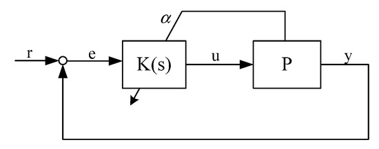
Figure 1.
Linear Parameter Varying (LPV) control scheme.
Under a small disturbance, the closed loop system is stable if in Equation (2) is frozen at any value but may be unstable when the controller is scheduled. Analysis of this problem is as follows:
Consider a nonlinear plant
where is the corresponding function, subscript “” stands for plant. Suppose the LPV description of system Equation (4) through Jacobian linearization is
For generality, it can be assumed that . Obviously at an equilibrium point (correspondingly,), the linearized model is
Its LPV controller is
where , according to Figure 1.
Assume the steady state system variables in Equation (4) and its controller Equation (7) can be parameterized by the parameter , which gives , , , and . Note that subscript “” stands for steady states throughout the paper. Define
Linearization of the controller Equation (7) gives
Substituting
into Equations (5) and (7) gives
and
respectively. Therefore, the close loop linearized system at this equilibrium point is
where
These matrices are different from those considered during conventional LPV synthesis, described as
The difference between and originates from the fact that the linearization of the controller Equation (7) should result in Equation (8), considering variation of scheduling parameter . The success of LPV synthesis applied to control aircrafts and missiles should owe to the fact that the directly transformed LPV model is a linear differential inclusion of the nonlinear system. However, a in Jacobian linearization-based LPV, such aa differential inclusion relation disappears. With the same controller, behavior of LPV model and that of the nonlinear plant is different.
3. Modification of Jacobian Linearization-Based LPV Control
It should be noted that the LPV model describes only the local dynamics near equilibrium points, so the designed controller should also be local. If LPV synthesis is performed on such LPV models, the purpose should be to meet the demand on local stability and performance at any equilibrium point. Therefore, should be time-invariant uncertainty during LPV synthesis.
To take the variation rate of into consideration, the LPV controller should also be viewed as a Jacobian linearization-based LPV of some nonlinear controller, i.e., should be written as Equation (12), not Equation (7).
Equation (12) is not a linear controller, because the definitions of and vary with . It is only a linearization description with parameterized system matrices just like that for the nonlinear plant. Directly implementing LPV controller Equation (7) on the nonlinear plant Equation (4) may result in unexpected close loop behaviors. It needs to find a corresponding nonlinear controller that has such a Jacobian linearization LPV formation such as Equation (12).
The question of whether such a nonlinear controller exists and how to find it will be discussed in the following section.
3.1. Definition of Controller
Theorem 1.
System
is a Jacobian linearization description of some nonlinear controller at the equilibrium point, if and only if there exists a pair of functions and that satisfy
for any value of . The corresponding nonlinear controllers can be described as
Theorem 2.
LPV controller Equation (7) for a Jacobian linearization-based LPV system has the linearization description Equation (13) at the equilibrium pointif and only if its parameterized steady state variablesandsatisfy the equation Equations (14) and (15) for any value of.
Proof of the theorems can be referred to in Appendix A and Appendix B.
3.2. Solution of Nonlinear Controller
Theorem 1 provides two equations, Equations (14) and (15), to solve for the desired nonlinear controller. The solvability analysis is given in the following. Assume . For Jacobian linearization-based LPV control, both and should be of the same dimensions as the controlled output, , i.e., and .
In Equations (14) and (15), separated equations need to be solved for separated derivatives. Therefore these partial derivatives can be determined uniquely. Then the primitive function and can be obtained if they exist. For the single input case, the primitive functions can always be found. For the multi-input case, the correlation between partial derivatives of a function may be violated, and consequently primitive function may not exist. As a result the desired nonlinear controller cannot be always found.
The procedure of improved LPV synthesis using a Jacobian linearization-based LPV is:
- (1)
- solving parameterized steady state system variable and using Equations (14) and (15);
- (2)
- using the modified LPV controller Equation (16) instead of Equation (7) to control the plant.
3.3. Discussion
It can be seen that the solution of Equations (14) and (15) depends on , which is determined by the plant. Generally, and cannot satisfy the steady state equation and Equations (14) and (15) simultaneously, so conventional LPV synthesis Equation (7) cannot be applied to the Jacobian linearization-based LPV model directly. This problem is essentially induced by deficient consideration of scheduling factor . The conventional LPV controller assumes to be stable near steady-state points. However, in dynamic processes, scheduling factor changes all the time. So, the traditional LPV controller only ensures local performance around steady-state points. When it works under conditions in which parameters change relatively fast, the controlling performance would be triggered.
In comparison, the improved LPV synthesis considers variation of in the varying equilibrium point . The modified LPV controller is designed around the varying equilibrium point , so it can provide satisfying controlling performance in a wilder operating region. In other words, the method proposed in this paper is a modification of the conventional LPV synthesis method.
Furthermore, there are also some special cases in which conventional LPV synthesis is reliable as listed below:
Case 1: the LPV controller that can be arranged as in Figure 2, from which an integrator can be isolated.
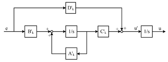
Figure 2.
Special LPV controller that needs no modification.
In this case, the controller can be described by
The parameterized steady state variables are , . Therefore,, and the linearized model is
According to the theorems, conventional LPV synthesis meets the requirements. This case is not rare. For example, in an H∞ design to achieve zero a steady-state tracking error, integral dynamics are specially added. If these controllers are arranged and scheduled as in Figure 2 in application, then LPV synthesis will be enough to guarantee a reliable design.
Case 2: a plant with purely integral actuator dynamics. In this case,, , and therefore . According to the theorems, there is no need for modification.
4. Application to a Turbofan Engine
This improved gain scheduling method was evaluated on a low bypass ratio, double-spool turbofan. Gross thrust of the engine is 4 kN and fuel mass flow rate is 160 L/h at the design point. A Nonlinear Component Level (NCL) model was developed with thermodynamic relations. Compressor and turbine characteristic maps were derived from experimental data, and were in the form of look-up tables. Combustion efficiency and pressure losses were fitted by curves. By means of this simplified model, key parameters can be calculated. More detailed description about the model can be found in the author’s previous work [27].
Based on this NCL model, both an engine LPV model was developed, and an LPV controller was designed. The LPV model was built in a sea-level static condition through Jacobian linearization and polynomial fitting. Two state variables, (high pressure turbine rotation speed) and (fan rotation speed) are considered. is used to control the thrust. The input is fuel mass flow rate with actuator dynamics as
Small perturbation simulation was carried out on several steady-state working points of the model, and linear models of each working point were fitted. Then the LPV model of the engine was obtained by fitting the linear state space matrix. Therefore, the extended LPV model by the actuator dynamics is
where and are the system matrices of the engine’s LPV model. The input ranges from 40% to 98%, and correspondingly the output ranges from about 82% to 96%. The design objective is a zero steady-state tracking error with settling time less than 2 s. Two types of scheduled controller are investigated in this part.
4.1. PI Controller-Based Gain Scheduling
Using a single PI (proportional–integral) controller tuned at for the whole operation range may result in large overshoot at low power and slow response at high power. Figure 3 shows step responses for initial speed at 83%, 88%, 92% and 96%, respectively. Therefore gain scheduling is required. Here, traditional gain scheduling is adopted, and eight PI controllers are designed to cover the operation range.
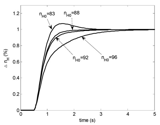
Figure 3.
Step responses with a single proportional–integral (PI) controller.
Gain and integrator in a PI controller can be arranged freely, for example, as in Figure 4 or Figure 5. Although they are equivalent in linear systems, scheduling of controllers yields nonlinearity and makes them different.
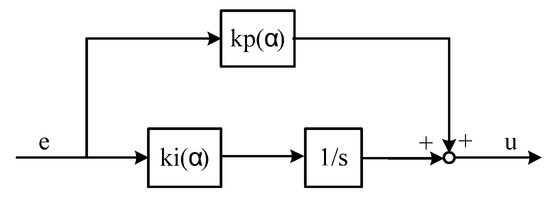
Figure 4.
PI gain scheduled controller: case 1.
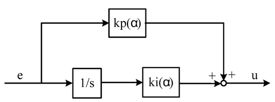
Figure 5.
PI gain scheduled controller: case 2.
If the PI controller is initially arranged and scheduled as in Figure 4, the system matrices are
and the steady state variables are
According to Theorem 2, the controller arranged as in Figure 4 can be designed following a conventional gain scheduling procedure. The scheduling will provide desired performance as displayed in Figure 6.
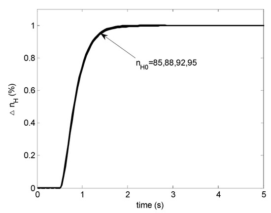
Figure 6.
Step responses with a scheduled PI controller: case 1.
Substituting
and
into Equations (A11) and (A12) in Appendix gives
which implies that does not depend on . For general scheduled PI controller designs, this cannot be satisfied and such a scheduled controller cannot work well without modification. As can be seen in Figure 7, the step responses exhibit undesirable behavior and the close loop system is even unstable at (not included in the figure).
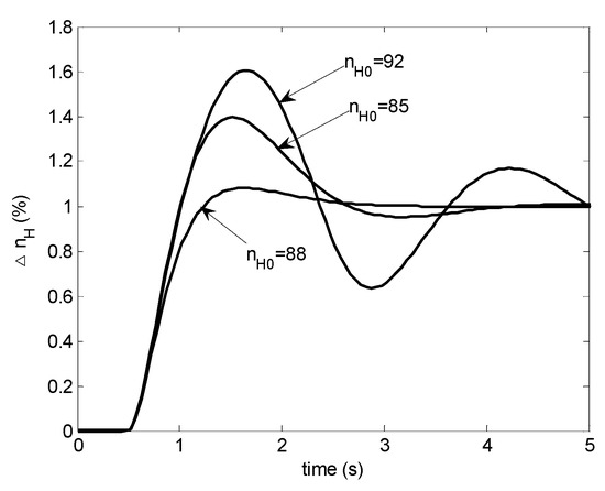
Figure 7.
Step responses with a scheduled PI controller: case 2.
To modify this controller, a pair of functions and should be solved from
which gives
To obtain from Equation (20), direct integration of the expression of should be avoided, as such an expression is usually much too complex. An alternative way is to first fit the numerical derivative by a polynomial, and then integrate the polynomial. Here, a 5th polynomial is used to fit . The results are plotted in Figure 8.
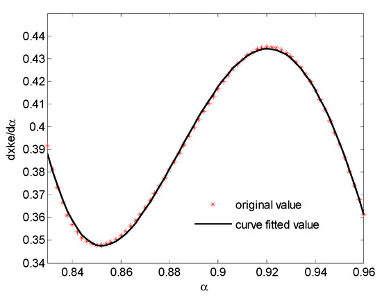
Figure 8.
Polynomial fitted result of .
The modified PI-based scheduling controller is shown in Figure 9. With this modified controller, the desired performance is achieved as shown in Figure 10, which agrees very well with Figure 6. It can been seen that the fitting result is good but not perfect. In our simulations, if a 3rd polynomial is used in the fitting, the goodness of fit is much worse but still can provide similar control performance to those shown in Figure 10. Therefore, the design result is not very sensitive to the solution inaccuracy of .
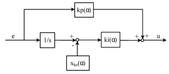
Figure 9.
Modified PI gain scheduled controller.
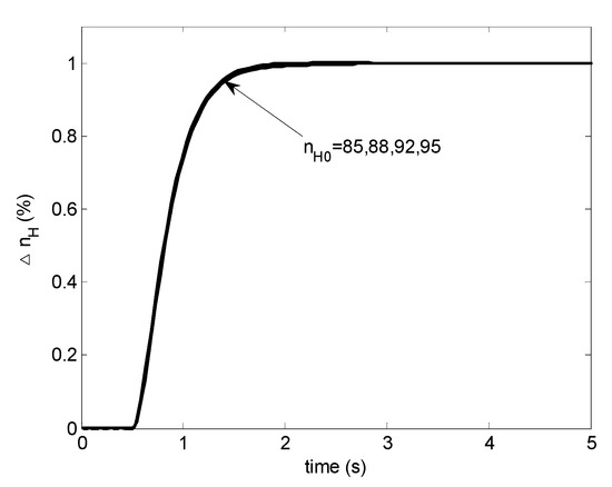
Figure 10.
Step responses with a modified scheduled PI controller.
4.2. H∞ Robust LPV Control
To control a general LPV plant, a linear time-invariant controller is required to be designed for a corresponding possible value of . For the turbofan engine in this paper, the gridding method is used.
In H∞ robust control, the system robustness and desired performance are achieved through weighting function specifications. Weighting functions consist of a sensitivity weighting function and a complementary sensitivity weighting function . should be large at low frequency, to obtain good disturbance attenuation and a small steady state tracking error. is shaped to be large at high frequency, in order to guarantee system robustness to un-modeled high frequency dynamics. and should be designed as first-order lags and leads, respectively.
Here, the unity-gain crossover frequency of is 0.4 rad/s.’s static gain needs to be adequately small, and the unity-gain crossover frequency is 100 rad/s. Following the above specifications, choose the weighting functions as
The H∞ controller design is performed at conditions of from 88% to 96% gridded with intervals of 0.5% for the extended LPV model Equation (19). As expected, the H∞ controller obtained has an order of five, the same as that of the augmented system. The controller is then reduced to order three while still providing acceptable performance. Then the controller is reformed to a controllable canonical form with system matrices as
With this reformation, only six parameters are scheduled. The H∞ controller scheduled conventionally does not provide acceptable step responses as shown in Figure 11. In the condition of lower than 83% or higher than 95%, the system is unstable and the corresponding step responses are not shown.
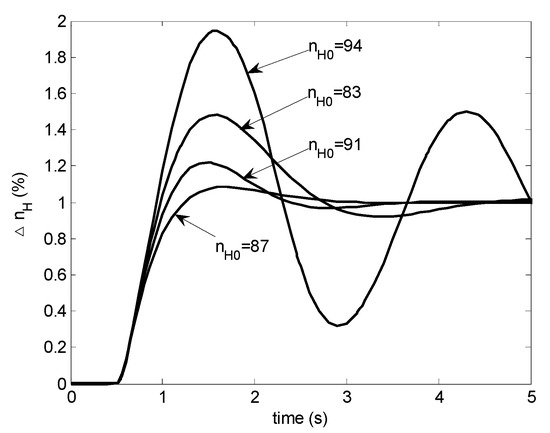
Figure 11.
Step responses with H∞ LPV controller.
Modification of this scheduled controller requires solving of the following equation according to Section 3.1:
The solution is
For simplicity, and are set to be zeros. and are obtained in the same way as in the modification for the PI-based scheduling controller. The resulting scheduled H∞ controller is shown in Figure 12. Fitted results of and by 4th and 5th polynomials, respectively, are plotted in Figure 13.
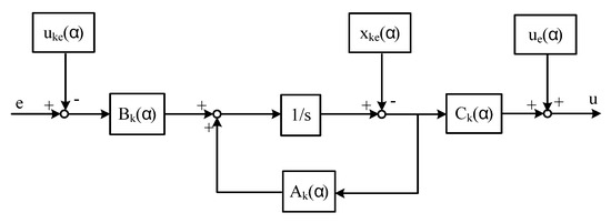
Figure 12.
Modified H∞ LPV controller.
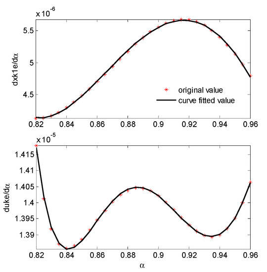
Figure 13.
Polynomial fitted result of and .
This modified LPV controller provides desired performance as shown in Figure 14, nearly the same as Figure 15 which is achieved by a group of H∞ controllers frozen at the corresponding operating conditions. For the condition of at 91%, it seems to be a little slower. Detailed examination reveals that the linearized model is not perfectly fitted by the LPV plant model in this condition. Therefore, it is not a problem with the modified scheduling approach.
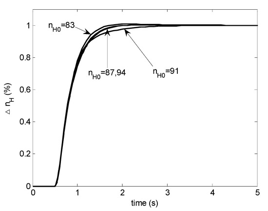
Figure 14.
Step responses with the modified H∞ LPV controller.
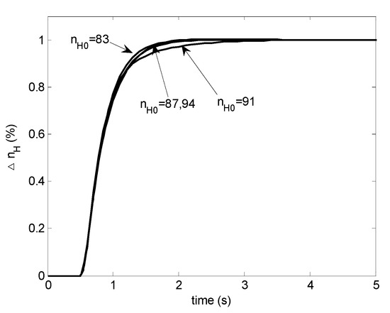
Figure 15.
Step responses with the frozen-parameter H∞ controller.
To avoid modification work, H∞ controllers should be designed and realized as in Figure 2. The weighting function is slightly changed to
to produce a pure integrator in the H∞ synthesis result. Again 5th order H∞ controllers are obtained. This time the controllers can only be reduced to 4th order without performance degradation. The controller other than the pure integral part is again reformed to controllable canonical form with six parameters to be scheduled. Satisfactory performance can be seen in Figure 16 with minor differences from Figure 14.
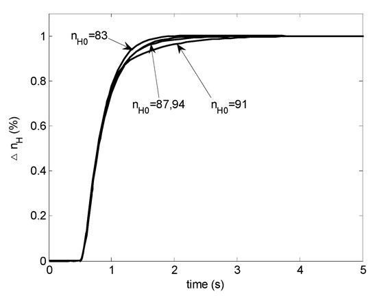
Figure 16.
Step responses with the H∞ LPV controller containing a pure integral part.
4.3. Discussion
In the above design examples, PI-based scheduling controller is a traditional gain scheduling design, while the H∞-based LPV is a more advanced one. For both of them, it is shown that although linear time-invariant controllers work well at any design point, a conventional scheduling of these controllers may yield unacceptable performance or even instability. The failure owes to the parameter variation in the controller. Although LPV synthesis can take the parameter variation into account, the variation rate of should be small enough. It can be verified that a constant Lyapunov matrix can always be found to satisfy
for any small enough varying range of . This implies that the result should guarantee required H∞ performance for arbitrary fast varying according to the LPV synthesis. In fact even the stability is not guaranteed as can be seen from the above simulations.
On the contrary, LTI controllers are designed separately during the above H∞ LPV design, i.e., the parameter-dependent Lyapunov function is used with no consideration of the variation of . With our improved design procedure, both stability and performance are achieved.
When LPV synthesis is implemented through the gridding method, it seems not much different to the traditional gain scheduling. It is impressive that the PI controller can serve as a good structure for gain scheduling design if special attention is paid to the arrangement of its components. Unfortunately, this regularly used design method was not well discussed before our research.
5. Conclusions
Gain scheduling is widely used as a nonlinear control strategy for aero-engines. The problem of traditional gain scheduling has been well discussed and LPV synthesis comes to be a more promising gain scheduling technique. For aero-engines, Jacobian linearization is adopted to build the LPV model for LPV synthesis. Theoretical analysis and simulation study both reveal that the well-established LPV synthesis may also fail to provide reliable stability and performance because it does not take the variation rate of scheduling parameters into consideration.
To solve this problem, the paper describes the controller as a Jacobian linearization-based LPV description and introduces two theorems to search for a solution to this nonlinear controller. The method essentially describes equilibrium points as a function of varying scheduling parameters, and designs a modified LPV controller around the varying equilibrium points.
Unlike traditional LPV controllers that only work well in a small region near a series of fixed equilibrium points, the modified controller can provide satisfying performance in a successive wilder operating region. It describes the nonlinearity of system more precisely.
The proposed method is applied to the controlling of a turbofan engine. Both the improved gain scheduling controller and improved H∞ robust LPV controller achieve reliable performance, which the proves effectiveness of the method.
Although the improved LPV synthesis proposed in this paper can attain a theoretical guarantee on stability and performance, the modification procedure inevitably increases the design task. So, the paper discusses some cases where the conventional gain scheduling method is mathematically equivalent to the improved method. In these cases, traditional gain scheduling will also work well, and gain scheduling control can be more easily implemented without modification work.
Author Contributions
Conceptualization, J.L. and D.Y.; Investigation, Y.M. and L.Z.; Methodology, J.L. and H.Z.; Software, Y.M. and L.Z.; Supervision, J.L. and H.L.; Validation, Y.M. and L.Z.; Writing—Original draft, H.Z.; Writing—Review and Editing, Y.M. and L.Z. All authors have read and agreed to the published version of the manuscript.
Funding
This research was funded by National Natural Science Foundation of China, grant number 51976042 and National Science and Technology Major Project, grant number 2017-V-0005-0055.
Acknowledgments
The authors would like to thank the anonymous reviewers for their valuable suggestions to refine this work.
Conflicts of Interest
The authors declare no conflict of interest.
Appendix A
Theorem A1.
System
is a Jacobian linearization description of some nonlinear controllers at the equilibrium point, if and only if there exists a pair of functionsandthat satisfy
for any value of. The corresponding nonlinear controllers can be described as
Proof.
(Necessity) Consider a nonlinear controller
Define
The linearization of (A5) at the equilibrium point gives
If the controller (A5) has the linearization description (A1), then
must hold.
In a steady state, partial derivation of the steady state equation
to gives
So (A2) holds. (A3) can be proved in the same way.
(Sufficiency) Define
Obviously
and
Using (A2), we have
Therefore, at the equilibrium point , nonlinear system
has a linearization description
The second equation in Equation (A4) can be proved in the same way. Therefore when Equations (A2) and (A3) are satisfied, Equation (A4) is the required nonlinear controller. □
Appendix B
Theorem A2.
LPV controller
for a Jacobian linearization-based LPV system has the linearization description Equation (A10) at the equilibrium pointif and only if its parameterized steady state variableandsatisfy the Equations (A2) and (A3) for any value of.
Proof.
(Necessity) Linearization of Controller Equation (A10) at equilibrium point gives
If controller Equation (A10) has a linearization description as Equation (A1), then
According to the Equations (A8), equation (A2) holds. Similarly, Equation (A3) holds.
(Sufficiency) According to Theorem 1, if Equations (A2) and (A3) hold for the LPV controller Equation (A10), then nonlinear controller Equation (A4) have the linearization description Equation (A9). Substituting the steady state equation
into Equation (A4) yields Equation (A10), which means system Equation (A10) has a linearization description as Equation (A1) at the equilibrium point . □
References
- Jaw, L.C.; Mattingly, J. Aircraft Engine Controls; American Institute of Aeronautics and Astronautics: New York, NY, USA, 2009; pp. 289–298. [Google Scholar]
- Weiser, C.; Ossmann, D.; Looye, G. Design and flight test of a linear parameter varying flight controller. CEAS Aeronaut. J. 2020, 11, 955–969. [Google Scholar] [CrossRef]
- Samar, R.; Postlethwaite, I. Design and Implementation of a Digital Multimode H∞ Controller for the Spey Turbofan Engine. ASME J. Dyn. Syst. Meas. Control 2010, 132, 64–71. [Google Scholar] [CrossRef]
- Sato, M.; Peaucelle, D. Gain-scheduled output-feedback controllers using inexact scheduling parameters for continuous-time LPV systems. Automatica 2013, 49, 1019–1025. [Google Scholar] [CrossRef]
- Pakmehr, M.; Fitzgerald, N.; Feron, E.M.; Shamma, J.S.; Behbahani, A. Gain scheduled control of gas turbine engines: Stability and verification. J. Eng. Gas Turbines Power 2014, 136. [Google Scholar] [CrossRef]
- Liu, Z.; Gou, L.; Fan, D.; Zhou, Z. Design of Gain-Scheduling Robust Controller for Aircraft Engine. In Proceedings of the 2019 Chinese Control Conference (CCC), Guangzhou, China, 27–30 July 2019. [Google Scholar]
- Yazar, I.; Kiyak, E.; Caliskan, F.; Karakoc, T.H. Simulation-based dynamic model and speed controller design of a small-scale turbojet engine. Aircr. Eng. Aerosp. Technol. 2018, 2, 351–358. [Google Scholar] [CrossRef]
- Shamma, J.S. Analysis and Design of Gain Scheduled Control. Ph. D. Thesis, Massachusetts Institute of Technology, Cambridge, MA, USA, 1988. [Google Scholar]
- Lu, B.; Wu, F.; Kim, W.S. Switching LPV control for high performance tactical aircraft. In Proceedings of the AIAA Guidance, Navigation, and Control Conference and Exhibit, Providence, RI, USA, 16–19 August 2004. [Google Scholar]
- Abbas, H.S.; Hanema, J.; Tóth, R.; Mohammadpour, J.; Meskin, N. An improved robust model predictive control for linear parameter-varying input-output models. Int. J. Robust Nonlinear Control 2018, 28, 859–880. [Google Scholar] [CrossRef]
- Abdalla, M.; Shaqarin, T. Industrial Process Control Using LPV. Mod. Appl. Sci. 2017, 11, 39–50. [Google Scholar] [CrossRef]
- Jia, Q.; Shi, X.; Li, H.; Han, X.; Xiao, H. Multivariable robust gain scheduled LPV control synthesis of turbofan engine. In Proceedings of the 2017 8th International Conference on Mechanical and Aerospace Engineering (ICMAE), Prague, Czech Republic, 22–25 July 2017. [Google Scholar]
- Emedi, Z.; Karimi, A. Fixed-structure lpv discrete-time controller design with induced l 2-norm and h 2 performance. Int. J. Control 2016, 89, 494–505. [Google Scholar] [CrossRef]
- Du, X.; Sun, X.M.; Wang, Z.M.; Dai, A.N. A scheduling scheme of linear model predictive controllers for turbofan engines. IEEE Access 2017, 5, 24533–24541. [Google Scholar] [CrossRef]
- Gilbert, W.; Henrion, D.; Bernussou, J.; Boyer, D. Polynomial LPV synthesis applied to turbofan engines. Control Eng. Pract. 2010, 18, 1077–1083. [Google Scholar] [CrossRef]
- Pan, M.; Zhang, K.; Chen, Y.H.; Huang, J. A New Robust Tracking Control Design for Turbofan Engines: H∞/Leitmann Approach. Appl. Sci. 2017, 7, 439. [Google Scholar] [CrossRef]
- Dong, Y.; Zhao, J. H∞ output tracking control for a class of switched LPV systems and its application to an aero-engine model. Int. J. Robust Nonlinear Control 2017, 27, 2102–2120. [Google Scholar] [CrossRef]
- Liu, T.J.; Du, X.; Sun, X.M.; Richter, H.; Zhu, F. Robust tracking control of aero-engine rotor speed based on switched LPV model. Aerosp. Sci. Technol. 2019, 91, 382–390. [Google Scholar] [CrossRef]
- Yang, D.; Zhao, J. H∞ bumpless transfer for switched LPV systems and its application. Int. J. Control 2019, 92, 1945–1958. [Google Scholar] [CrossRef]
- Huang, X.; Wu, C.; Liu, Y. Finite-Time H∞ Model Reference Control of SLPV Systems and its Application to Aero-Engines. IEEE Access 2019, 7, 43525–43533. [Google Scholar] [CrossRef]
- Xiong, J.; Cheng, Z.; Gao, J.; Wang, Y.; Liu, L.; Yang, Y. Design of LPV Control System Based on Intelligent Optimization. In Proceedings of the 2019 Chinese Control and Decision Conference (CCDC), Nanchang, China, 3–5 June 2019; pp. 2160–2165. [Google Scholar] [CrossRef]
- Qian, Y.; Ye, Z.; Zhang, H.; Zhou, L. LPV/PI Control for Nonlinear Aeroengine System Based on Guardian Maps Theory. IEEE Access 2019, 7, 125854–125867. [Google Scholar] [CrossRef]
- Rosa, P.; Silvestre, C.; Cabecinhas, D.; Cunha, R. Auto landing Controller for a Fixed Wing Unmanned Air Vehicle. AIAA Paper 2007, 6770. [Google Scholar] [CrossRef]
- Bruzelius, F.; Pettersson, S.; Breitholtz, C. Linear Parameter-Varying Descriptions of Nonlinear Systems. In Proceedings of the American Control Conference, Boston, MA, USA, 30 June–2 July 2004; pp. 1374–1379. [Google Scholar]
- Reberga, L.; Henrion, D.; Bernussou, J.; Vary, F. LPV Modeling of a Turbofan Engine. In Proceedings of the 16th IFAC World Congress, Prague, Czech Republic, 3–8 July 2005; 2005; pp. 3–8. [Google Scholar]
- Leith, D.J.; Leithead, W.E. On Formulating Nonlinear Dynamics in LPV Form. In Proceedings of the 39th IEEE Conference on Decision and Control, Sydney, Australia, 12–15 December 2000; pp. 3526–3527. [Google Scholar]
- Zhao, H.; Liu, J.; Yu, D. Approximate Nonlinear Modeling and Feedback Linearization Control for Aeroengines. J. Eng. Gas Turbines Power 2011, 133. [Google Scholar] [CrossRef]


Publisher’s Note: MDPI stays neutral with regard to jurisdictional claims in published maps and institutional affiliations. |
© 2020 by the authors. Licensee MDPI, Basel, Switzerland. This article is an open access article distributed under the terms and conditions of the Creative Commons Attribution (CC BY) license (http://creativecommons.org/licenses/by/4.0/).