Abstract
Vapor compression systems (VCS) cover a wide range of applications and consume large amounts of energy. In this context, previous research identified the optimization of the condenser fans speed as a promising measure to improve the energy efficiency of VCS. The present paper introduces a steady-state modeling approach of an air-cooled VCS to predict the ideal condenser fan speed. The model consists of a hybrid characterization of the main components of a VCS and the optimization problem is formulated as minimizing the total energy consumption by respectively adjusting the condenser fan and compressor speed. In contrast to optimization strategies found in the literature, the proposed model does not relay on algorithms, but provides a single optimization term to predict the ideal fan speed. A detailed experimental validation demonstrates the feasibility of the model approach and further suggests that the ideal condenser fan speed can be calculated with sufficient precision, assuming constant evaporating pressure, compressor efficiency, subcooling, and superheating, respectively. In addition, a control strategy based on the developed model is presented, which is able to drive the VCS to its optimal operation. Therefore, the study provides a crucial input for set-point optimization and steady-state modeling of air-cooled vapor compression systems.
1. Introduction
Vapor compression systems (VCS) are used in many technical applications, such as the air conditioning of buildings, food temperature control, automotive applications, etc., and consume a considerable amount of energy. For instance, air conditioning and refrigeration account for about 24% of household energy consumption in the USA [1] and for hot and high humid countries like Singapore this consumption can represent over 50% [2]. Therefore, increasing the energy efficiency of VCS through optimization and control appears to be a key issue [3]. One prospective possibility for energy saving is the quasi-stationary control, which aims to achieve the highest possible efficiency within one operating condition, i.e., set-point optimization.
1.1. Ideal Condenser Fan Speed
According to Jensen and Skogestad [4], the optimal energy efficiency of a VCS can be obtained by adjusting the five degrees of freedom: refrigerant mass flow rate, superheating, subcooling, condensing, and evaporating pressure. These theoretical degrees of freedom can be influenced by the actuators of the given system. Considering a conventional air-cooled chiller with a thermostatic expansion valve (TXV), as shown in Figure 1, the compressor and condenser fan speed are available actuators to set the five degrees of freedom. Hence, an infinite number of combinations of the compressor and condenser fan speed can meet the load demand, but with different energy efficiency [5,6]. Thereby, the energy efficiency can be quantified by the coefficient of system performance
where , , and are refrigeration capacity, compressor power, and condenser fan power. The optimization problem of the ideal condenser fan speed occurs because of a tradeoff between the compressor and fan power consumption [5]. For instance, rising fan speed increases the fan power consumption, but decreases the condensing pressure due to higher heat rejection, which in turn leads to lower compression work. Figure 1 shows the power consumption of compressor, fan, and the sum of both against the fan speed at constant cooling load, coolant inlet temperature (), and condenser air inlet temperature () to illustrate the tradeoff.
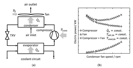
Figure 1.
Air-cooled vapor compression system (VCS) comprising compressor, condenser, thermostatic expansion valve (TXV), evaporator, and condenser fan (a). Electric power of the condenser fan, compressor, and the sum of both for constant air inlet temperature, coolant temperature, and refrigeration capacity. The characteristic of the compressor and condenser fan power results in an energy efficiency optimum. A low curvature in the vicinity of the minimum can be observed (b).
The ideal condenser fan speed exhibits a strong dependence on the ambient temperature and the refrigeration capacity [7,8]. Consequently, the speed of the condenser fan must be adjusted in accordance with the operating conditions in order to achieve optimum performance.
1.2. Optimization of the Condenser Fan Speed Control
A key aspect of the condenser fan speed optimization is the VCS modeling, which can be separated into black box and component-based [9]. While black box models use a set of data to characterize the system, component-based models consider physical aspects for describing each component of the system. Furthermore, component-based models can be subdivided regarding the heat exchanger modeling into empirical, distributed, moving boundary, and hybrid or lumped models [10,11]. An overview of steady-state VCS modeling is given by Wan et al. [9] and Zhang et al. [12]. The VCS models are usually assessed on the basis of the prediction accuracy of the coefficient of performance (COP). In this context, Scarpa et al. [13] have stated that the most accurate models lead to a COP estimation error of ±5%, and ±10% can be considered as a high level of accuracy. In fact, the most models for set-point optimization perform a COP estimation accuracy of about ±10% [14,15,16,17,18,19,20].
Using different modeling approaches, various optimizing system controls of varying complexity are proposed in the literature [21,22]. As a simple solution, the ideal condenser fan speed can be determined in advance to derive a linear function [7,8] or a regression [19,23] for control. In 2004, Chan and Yu [8] published a control of the condensing temperature as a linear function of the ambient temperature. In a further publication, Yu and Chang [19] suggested a load-based speed control for a small ambient temperature range. These solutions can provide a significant improvement compared to the traditional constant condensing pressure control, but only achieve suboptimal results for different operating conditions of ambient temperature and cooling load [7,8]. Larsen et al. [24] proposed a linear, online control of the VCS, which calculates the ideal settings iteratively via gradient method and thus obtains high energy efficiency for various operating conditions. Thereby, the condenser fan and compressor speed are considered as actuators. The applied hybrid model is verified by measurements on a supermarket refrigeration system. Although some rough assumptions are made in terms of a lump condenser model and constant compressor efficiency, high accuracy is achieved when calculating the ideal settings. As a drawback of this method, a long time (over 50 min [7]) is required to drive the system to ideal operation. Zhao et al. [10] and Ruz et al. [17] presented steady-state optimization strategies based on the hybrid heat exchanger model suggested by Ding et al. [25]. Zhao et al. used a modified genetic algorithm to obtain optimum set-points, minimizing the total operating costs of the compressor, evaporator fan, and condenser fan. Ruz et al. iteratively optimized the settings of a VCS to achieve the ideal condenser pressure and expansion valve opening. Huang et al. [26] also used a hybrid model to develop an optimizer that incorporates the speed of the compressor, condenser fan, and evaporator fan of an automotive air conditioning system. Further studies employ artificial neuronal networks (ANN) [18,20], sate space modeling [27], exergy-based models [28], and semi-empirical models [16] to predict the ideal condenser fan speed. In addition to these model-based methods, the model-free method of extremum seeking control is discussed for the set-point optimization of VCS [29,30]. The extremum seeking control is a very prospecting solution, since no advanced component models are required. On the other hand, the disadvantages include a long convergence time, until an ideal operation is achieved and there are no predictive capabilities [22].
The most set-point optimization strategies deal with more than condenser fan and compressor speed optimization [10,16,17,18,26,27,28], resulting in complicated cross-coupling, especially due to superheating and evaporating pressure [31,32]. Therefore, the published model-based set-point optimization strategies generally need complicated algorithms, whereas black models always require detailed data from measurements for the validation and training [13]. In addition, most solutions for set-point optimization need considerable time to achieve the ideal settings [7,29,30]. To the authors’ knowledge, no method has yet been published that predicts the ideal condenser fan speed according to a single optimization term.
The main contribution of the present paper is the introduction of a model-based optimization method for a fast and simple determination of the ideal condenser fan speed under stationary operating conditions. Therefore, a new hybrid model approach is developed to derive a single optimization term. The optimization problem is formulated as minimizing energy consumption of the condenser fan and the compressor subject to constant refrigeration capacity and ambient temperature. To demonstrate the feasibility, a detailed model validation is carried out of 250 measuring points and the model assumptions are discussed. The influences of several parameters on the ideal condenser fan speed are studied to contribute to the understanding of the model accuracy, although some rough simplifications are made. In addition, a control strategy based on the model approach is suggested.
2. Experimental Methodology
Experimental tests have been conducted on an air-cooled vapor compression system to verify the hybrid model proposed in this research. The test setup, calculation backgrounds, and the experimental procedure are described in order to provide an appropriate basis for the interpretation of the findings.
2.1. Test Bench Description
The test specimen of the present study is a serial battery cooling unit of the Mahle GmbH [33]. The system works as an air-cooled vapor compression system and consists of a refrigerant-coolant evaporator (chiller), a suction gas-cooled electric scroll compressor, an air-refrigerant condenser with integrated receiver and dryer, an axial condenser fan, and a thermostatic expansion valve (TXV). The working fluid is a mixture of R134a and polyalkylene glycol (PAG) synthetic oil. A description of the VCS components is detailed in Table A1. The VCS is instrumented with temperature () and pressure () sensors before and after each component. In the liquid line, the speed of sound () is measured to calculate the oil fraction and a Coriolis sensor is equipped to detect the refrigerant mass flow rate (). Furthermore, voltage (,), current (,), and speed (,) are recorded at the compressor and condenser fan, respectively. A picture of the instrumented battery cooling unit is highlighted in Figure A1. The experimental setup of the test specimen and the corresponding test bench is detailed in Figure 2.
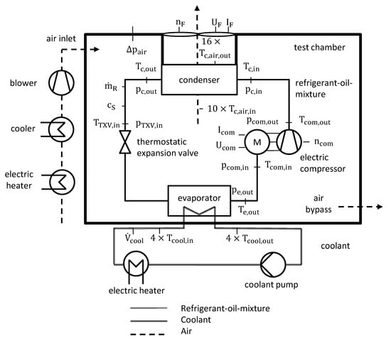
Figure 2.
Schematic overview of the experimental setup. The VCS is placed in an air-conditioned test chamber. The VCS is instrumented with sensors to measure the temperature (), pressure (), speed of sound (), and refrigerant mass flow rate () of the VCC, as well as the speed (), current (), and voltage () of the compressor and condenser fan. A temperature and volume flow rate ()-controlled coolant flow is provided at the evaporator.
The VCS itself is placed in an air-conditioned test chamber. Thereby, an electric air heater and a cooler are employed to control the air temperature in the chamber. The air temperature is measured at the inlet () and outlet () of the condenser. The blower of the test bench supplies the conditioned air into the test chamber, while the air flow through the condenser is provided by the condenser fan of the VCS. To ensure a free suction of the condenser fan, the pressure difference () between the test chamber and the environment is monitored and controlled. The secondary mass flow rate through the evaporator is a coolant (50/50 mas.-% water/glycol), which is provided by the coolant pump of the test bench and measured magnetic-inductively (MID). The temperature of the coolant is monitored at the inlet () and outlet () by three calibrated type K thermocouples and one Pt100 sensor, respectively. An electric heater is installed in the coolant circuit to adjust the coolant temperature.
2.2. Calculation Background
For the assumption of an isenthalpic expansion, the refrigeration capacity
can be balanced on the refrigerant side of the evaporator, where , , and are refrigerant mass flow rate, enthalpy at the evaporator outlet, and at the thermostatic expansion valve (TXV) inlet, respectively. The refrigerant mass flow rate is a direct measured value provided by the Coriolis sensor, whereas the enthalpies must be calculated on the basis of the pressure, temperature, and oil percentage. Therefore, the specific enthalpy of the refrigerant-oil-mixture
is determined with respect to Youbi-Idrissi et al. [34] as a function of the oil content of the total mass flow , the steam fraction related to the total mass flow , the refrigerant enthalpy of liquid and vapor , the oil enthalpy , and the excess enthalpy (describing the mixing enthalpy of the refrigerant-oil-mixture) [34]. The enthalpy values are taken from Span et al. [35] and measurements of the ILK Dresden mbH on behalf of the Mahle Gmbh [36]. The oil percentage
can be calculated using a polynomial of temperature, pressure, and sound velocity [37]. The coefficients of the polynomial are carried out by ILK Dresden mbH on behalf of the Mahle GmbH [38]. Based on the aforementioned considerations, the coefficient of system performance can be identified according to Equation (1). Thereby, the compressor and fan power are calculated by the product of the measured current and voltage.
The uncertainty of the measurement chain is developed according to the type B of the “Guide to the expression of uncertainty in measurement” (GUM) [39]. Detailed information about the sensors and their corresponding uncertainty are listed in Table A2 and Table A3. The extended measurement uncertainty (coverage factor of k = 2) of the derived quantities are calculated with respect to the Gaussian error propagation. Detailed information on the measurement uncertainty calculation is described by Angermeier et al. [40].
2.3. Experimental Procedure and Test Matrix
The energy efficient operation of the VCS is investigated for fifteen different set-points, which are oriented to the specifications of battery cooling units for electric buses. The considered set-points are listed in Table 1.

Table 1.
Boundary conditions for fifteen set-points regarding the refrigeration capacity, condenser air inlet temperature, and evaporator coolant inlet temperature.
Subject to the conditions in Table 1, each set-point is measured for several combinations of compressor and condenser fan speed to investigate the effect on the coefficient of system performance (COSP). In sum, 250 steady-state measuring points are conducted. Thereby, a stationary measuring point is defined for fluctuations below ±0.1 K and ±50 W for the temperatures of the secondary fluids (air and coolant) and the refrigeration capacity, respectively. Within one set-point, the air volume flow rate through the condenser is changed by about 100 rpm of the condenser fan speed between different measuring points. At the same time, the compressor speed is adjusted to maintain a constant refrigeration capacity. In this way, the determination of the COSP is covered for the entire application range of the air-cooled VCS to identify the ideal condenser fan speed of a given set-point. Thereby, the ideal condenser fan speed for a set-point is specified as the fan speed leading to the highest COSP. The results of the COSP and the associated measurement uncertainty for one set-point are presented in Figure 3. As reported in literature, a flat optimum of the COSP to the condenser fan speed can be observed. With respect to the uncertainty in measurement, only a range of fan speeds can be defined as ideal. Consequently, a range of ±300 rpm is considered to be ideal in this research.
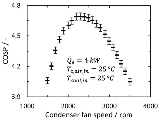
Figure 3.
The coefficient of system performance (COSP) for varying condenser fan speed within a constant set-point of 4 kW refrigeration capacity, 25 °C ambient air temperature and coolant temperature. The error bars define the uncertainty in determining the COSP and indicate a range of ±300 rpm as the ideal condenser fan speed, due to the low curvature around the optimum.
3. Mathematical Model
The mathematical model is developed for steady-state conditions and is based on a hybrid characterization of the air-cooled VCS components. Thereby, the model aims to obtain a tradeoff between accurate prediction of the ideal condenser fan speed and low calculation effort.
3.1. Calcualtion Procedure
The required model input parameters are the refrigeration capacity (), ambient air temperature (), evaporating pressure (), superheating (), subcooling (), thermophysical properties of the air and the refrigerant, and component specifications. For the model validation, a secondary mass flow rate through the condenser, i.e., air mass flow rate () can be inserted to calculate the condensing temperature (), condensing pressure (), refrigerant mass flow rate (), air outlet temperature of the condenser (), compression power (), fan power (), COP, and COSP. Thereby, the model outputs can be compared with the experimental results. In the case of the condenser fan speed optimization, all input parameters must be assumed to be constant within a single set-point. An overview of the calculation procedure is provided in Figure 4.
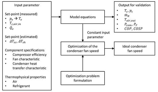
Figure 4.
Overview of the calculation procedure. Inputs are set-point specifications, component characteristics of the compressor, fan, and condenser heat transfer, as well as thermophysical properties of the air and the refrigerant. For the calculation of the ideal condenser fan speed, the input parameters are assumed to be constant.
3.2. Model Description
3.2.1. Condenser Fan
Assuming that the motor torque is a quadratic function of the fan speed and the speed is proportional to the air mass flow rate (), the fan power
can be calculated by the third power of the air mass flow rate and the combined fan specification .
3.2.2. Evaporator and Expansion Valve
No model of the evaporator heat transfer and the expansion valve is required due to the input of the refrigeration capacity, evaporating pressure, and superheating. Instead, an energy balance for the evaporator heat transfer rate
with an isenthalpic expansion is applied to derive a relation between the condensing temperature and the refrigerant mass flow rate. Thereby, , , are the mean specific heat capacity of subcooling, superheating, and boiling curve from evaporating to condensing pressure, , , , , are subcooling, superheating, evaporating and condensing temperature, and are specific evaporating enthalpy and refrigerant mass flow rate, respectively. The relationship is demonstrated in Figure 5.
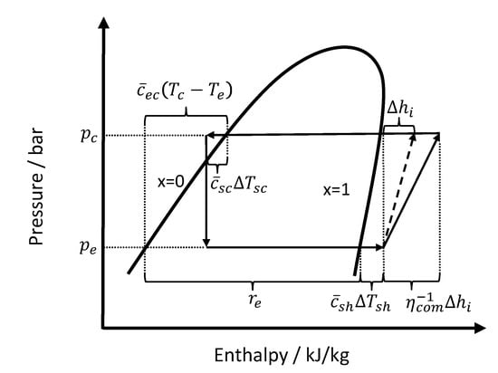
Figure 5.
Simplified log p-h diagram of the vapor compression cycle. The terms employed for the energy balance of the refrigeration capacity and the compression work are highlighted.
A modification of Equation (6) leads to the condensing temperature
as a function of the refrigerant mass flow rate, since the substitutions and merge model input parameters.
3.2.3. Compressor
The electric compression power
is a function of the compressor efficiency , refrigerant mass flow rate , and isentropic enthalpy difference (compare Figure 5). Neglecting the pressure losses due to superheating, desuperheating, condensing area, and between the heat exchangers and compressor, the isentropic enthalpy is defined as:
To find a reasonable solution for , the real gas behavior of the specific volume
described by the gas constant , real gas factor , temperature, and pressure is applied. For an isentropic state change, the product is fairly constant, and thus a possible approach for an isentropic state change is found:
A second expression of the refrigerant properties combines condensing pressure and temperature:
Further information of both approaches is provided in Appendix B. Inserting these relations into Equation (8) yields an equation for the compressor power
The combination of Equations (7) and (13) gives a linear expression of the compression power
as a function of the refrigerant mass flow rate and the combined input parameters and .
3.2.4. Condenser
For a simple characterization of the complex heat transfer of the condenser, a lumped number of transfer units (NTU) method is chosen. Considering a uniform wall temperature equal to the condensing temperature, and neglecting superheating and subcooling, the condenser heat flow
is given, where , , , , , and are the maximal possible condenser heat transfer, air mass flow rate, specific heat capacity of the air, air inlet temperature, heat exchanger characteristic, and the number of transfer units, respectively. Assuming thermal resistance is only determined by the air side heat transfer, the number of transfer units
of the condenser can be expressed according to Ding et al. [25], where is the overall heat transfer coefficient and is a constant that depends on the air properties and the heat transfer area. The exponent is a constant reflecting the flow characteristic of the heat exchanger. With respect to the external forced convection correlation of Zukauskas [41], the exponent is defined.
3.2.5. System
An energy balance of the overall cycle
reveals in combination with Equations (7) and (14), the coupling of the air and the refrigerant mass flow rate:
Therefore, the refrigerant mass flow rate
with the substitutions
of the input parameters, is a direct function of the air mass flow rate and the current set-point. Thus, a necessary term for the direct solution of the optimization problem is identified.
3.3. Formulation of the Condenser Fan Speed Optimization Problem
The optimization of the condenser fan speed intends to minimize the total energy consumption of the VCS at constant refrigeration capacity and secondary fluid outlet temperature at the evaporator, i.e., coolant outlet temperature . The mathematical formulation of the problem is:
with subject to
A reasonable solution is to derive the cost function according to the air mass flow rate of the condenser
and to set it to zero. The chain rule is obtained to calculate the derivation of the compression power to air mass flow rate. Assuming constant input parameters, the derivation
can be expressed using the model Equations (5) and (14). The coupling function derivation
is an implicit function of the air mass flow rate and the operating conditions, and its development is described in Appendix C. Subsequently, an implicit optimization term for the ideal air mass flow rate
is attained. Indeed, Equation (20) can easily be solved by fix point iteration in Matlab or Microsoft Excel, for example.
4. Model Validation
The model validation is demonstrated for the air-cooled VCS described in Section 2.1 and carried out of 250 steady-state measuring points. The deviation of the experimental and the model data are discussed for two different cases:
- Component model validation (varying model inputs)
- Condenser fan speed optimization validation (constant model inputs)
In detail, this means that for case 1, the input variables are taken from measurement, except the coefficient of the condenser heat transfer, i.e., and the refrigerant fitting parameters , , , which are constant, respectively. For the validation of the condenser fan speed optimization (case 2), all input parameters are constant within an operation point. Furthermore, the compressor efficiency, subcooling, superheating, and the specific heat capacities of the refrigerant are constant for all set-points. The evaporating pressure, temperature, and enthalpy vary between different set-points. By subdividing into case 1 and 2, the error sources can be evaluated for the components and the optimization scenario, separately. The maximal deviation, the relative root mean square error (R-RMSE), and the coefficient of determination are summarized in Table 2. The statistic calculation background is detailed in Appendix D.
Table 2.
Maximum deviation, R-RMSE, and coefficient of determination for the model approach. The first value is for varying model inputs (case 1) and the second for constant model inputs (case 2).
4.1. Condenser Fan
The condenser fan power prediction and the test data are plotted in Figure 6. A constant input of the fan characteristic induces a coefficient of determination and a maximal deviation of 99.67% and 0.02 kW, while a varying input of results in no error and is therefore not depicted. Evidently, the model describes the fan power with sufficient accuracy for a cycle analysis.
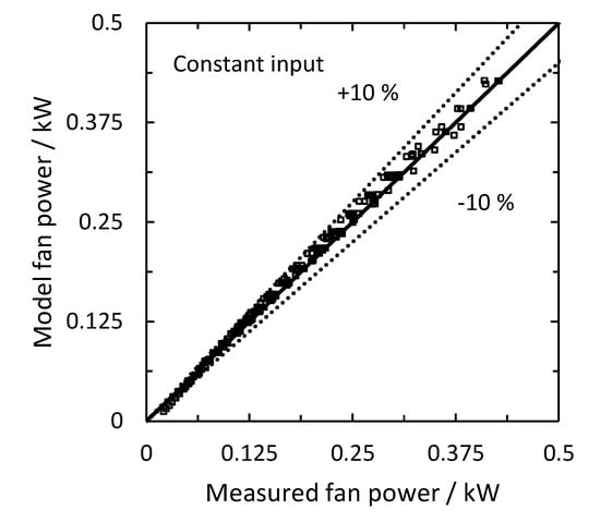
Figure 6.
Experimental validation of the condenser fan power for a constant fan characteristic .
4.2. Evaporator and Expansion Valve
The hybrid model in Section 3.2 neither includes an evaporator heat transfer model nor an expansion valve model, as the evaporating pressure and superheating are inputs of the model. Therefore, a reasonable validation of the assumptions for the expansion valve and the evaporator is the evaluation of the condensing temperature in Equation (7). The results for case 1 and 2 are presented in Figure 7.
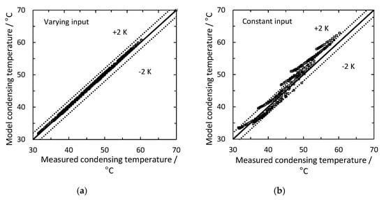
Figure 7.
Experimental validation of the evaporator and the expansion valve. (a): Varying input parameters (b): Constant input parameters. The accuracy decreases for constant input parameters.
A maximal deviation of 0.6 K, an R-RMSE of 0.72%, and a coefficient of determination of 99.93% are performed for varying input parameters. The discrepancy may be caused by the measurement uncertainty of the inputs and the assumption of an isenthalpic expansion. For a constant input, the error increases to a maximal deviation of 4.5 K, a R-RMSE of 4.36, and a of 97.07%, respectively. However, a sufficient prediction of the condensing temperature is obtained. Consequently, the input parameters in Equation (7), i.e., superheating, subcooling, evaporating pressure, and coolant load do not change significantly within a constant set-point or barely affect the condensing temperature. In fact, the main source of error for the VCS under consideration is the change in subcooling, whereas superheating and subcooling remain fairly constant.
4.3. Compressor
Figure 8 depicts the comparison of the compression power predicted by the model approach and measured in the experiments. For varying model inputs, the error due to the refrigerant model, condensing temperature calculation, and uncertainty in measurement of all input parameters are included. However, the main error is caused by the modeling of the specific volume, especially for higher pressure. In this context, the validation of refrigerant model is provided in Appendix B. Nevertheless, the refrigerant properties approach in Equations (11) and (12) is suitable for compression power calculation achieving a R-RMSE of 2.65% and a coefficient of determination of 99.69%. If constant input parameters are taken into account, the accuracy of the prediction deteriorates, particularly due to the constant compressor efficiency, but still leads to a coefficient of determination of 96.69% and thus can be used for system analysis. This finding is in good agreement with the results of Larsen [7], who also used constant compressor efficiency and came to the same conclusion carrying out the validation of a supermarket refrigerator.
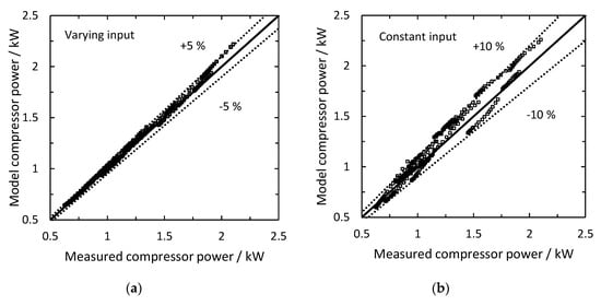
Figure 8.
Experimental validation of the compressor power. (a): Varying input parameters. (b): Constant input parameters. High prediction accuracy despite constant compressor efficiency.
4.4. Condenser
For the validation of the condenser heat transfer modeling, the air outlet temperature according to Chi and Didion [42]
can be employed. The results are highlighted in Figure 9. The measured condensing temperature is used as input in Equation (11) to provide an isolated consideration of the condenser model prediction error. Thereby, a R-RMSE and a coefficient of determination of 2.73% and 99.78% are performed, respectively. With respect to the expanded measurement uncertainty of 0.55 K of the air outlet temperature, a maximal deviation of 1.3 K reveals high accuracy despite rough assumptions.
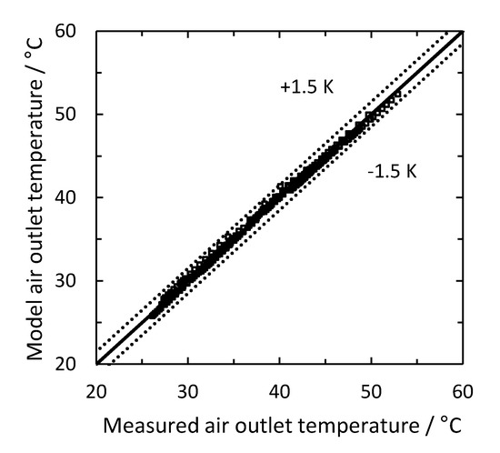
Figure 9.
Experimental validation of the condenser air outlet temperature. High accuracy despite rough assumptions is obtained.
4.5. System
Model predictions and test data of the refrigerant mass flow rate are provided in Figure 10. With respect to Equation (19), the mass flow rate calculation includes the errors due to the component modeling of the evaporator, compressor, and condenser. However, for varying input parameters, the coefficient of determination is 99.67%, and for constant inputs is 99.27%.
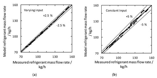
Figure 10.
Experimental validation of the refrigerant mass flow rate. (a): Varying input parameters. (b): Constant input parameters.
Figure 11 highlights the results for the model estimation and the test data of the COSP for varying and constant input parameters. The prediction errors of the component models superpose for the COSP calculation. Nevertheless, for varying input, a COSP prediction error within ±10% and a R-RMSE of 2.94% are obtained. Hence, the model can be considered as a model with good accuracy [13].
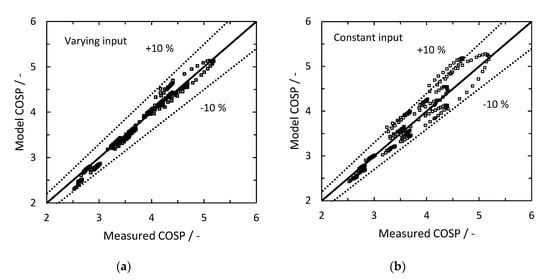
Figure 11.
Experimental validation of the COSP. (a): Varying input parameters. (b): Constant input parameters. The prediction accuracy decreases for constant input parameters.
On the other hand, the proposed hybrid model does neither simulate the evaporator heat transfer nor the expansion valve characteristics. As a consequence, the model requires the input of the evaporating pressure and superheating, which limits the comparability. However, for constant input, parameters over 93% of the predicted COSP are still within ±10% deviation and the R-RMSE is 6.12%. Therefore, the results are more accurate than the model results of Chan and Yu [6] or Braun et al. [16], for example. Moreover, the model is developed to predict the ideal condenser fan speed within a constant set-point, and in this respect, only small changes in evaporating pressure and superheating can be expected.
4.6. Prediction of the Ideal Condenser Fan Speed
The aim of the model approach in Section 3 is the prediction of the ideal condenser fan speed according to Equation (26). The results for the measured and the calculated ideal condenser fan speed are compared in Figure 12 and outline a deviation within a range of ±300 rpm, respectively. Considering the measurement uncertainty (compare Section 2.3), the predictions appear to be ideal in terms of energy efficiency for varying and constant input parameters.
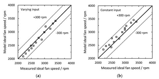
Figure 12.
Comparison of the measured and the calculated ideal condenser fan speed. (a): Varying input parameters. (b): Constant input parameters. The prediction accuracy is comparable for both cases and is within the uncertainty range of ±300 rpm.
Based on the results of the model validation in Section 4.5, the high accuracy for the varying input is not particularly surprising. In contrary, the estimation accuracy for the constant input may be surprising, bearing in mind that the COSP estimation error for constant and varying input in Figure 11 differs significantly. However, the results of the measured and the predicted COSP for a single set-point in Figure 13 point out that the absolute value of COSP vary for a constant input, whereas shape and position in terms of condenser fan speed are comparable. Consequently, some input parameters influence the prediction error with regard to COSP, but influence less the ideal fan speed. In order to explain this circumstance, the impacts of the input parameters are examined in the following.
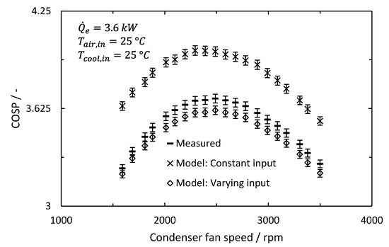
Figure 13.
Measured and predicted COSP of varying and constant input demonstrated for one set-point. The model input parameters influence the COSP, but hardly the ideal condenser fan speed.
5. Condenser Fan Speed Optimization
5.1. Influences on the Ideal Condenser Fan Speed
The ideal condenser fan speed is influenced by various variables, and according to Equation (26), all input parameters of the model in Figure 4 have an impact. Strong effects have already been reported for the ambient temperature and the refrigeration capacity, while the influences of the other values like the superheating, subcooling, compressor efficiency, and the suction pressure are not yet clear.
To investigate the effect of a parameter to the ideal air mass flow rate and consequently to the ideal condenser fan speed, the formulation of a sensitivity coefficient
with
can be defined. For a constant fan characteristic , the sensitivity coefficient
is yielded as a function of the current set-point, the parameter , and the ideal air mass flow rate. Thereby, Equation (30) clarifies that only a change of the gradient of the compressor power to the air mass flow rate impacts the ideal fan speed. The shape of the compression power in Figure 1 illustrates this gradient. It can be seen that an increase in the negative slope would move the ideal fan speed to higher values. The gradient itself depends on the heat transfer rate at the condenser, as an adjustment of the condenser fan speed is only reasonable from an energetic point of view, if the influence of the fan speed on the condensing pressure and thus on the compression power changes. Consequently, the ideal condenser fan speed changes solely, if the input parameter modifies the condensing pressure. Thereby, surging condensing pressure causes a higher ideal condenser fan speed. In general, it is fair to assume that the condensing pressure is more influenced by the ambient temperature and the refrigeration capacity than by the subcooling, superheating, compressor efficiency, or the evaporating pressure.
However, to quantify this general consideration, the validated model can be used. Therefore, the absolute change of the ideal condenser fan speed is investigated at one reference set-point and highlighted in Figure 14. Here, the adjustment scope of the input parameters is selected with regard to the operating range of the VCS under consideration. With respect to the input values, the total changes of the ideal fan speed are 1100 rpm, 620 rpm and 280 rpm for an increasing refrigeration capacity, ambient temperature, and evaporating pressure, respectively. Changing the compressor efficiency from 0.4 to 0.6 causes a fan speed adjustment of 220 rpm. This small effect is in line with previous results [7]. The modification of the lumped heat transfer coefficient of 30% leads to a change of the fan speed of 130 rpm. Even lower is the effect of the subcooling and the superheating with 120 rpm and 70 rpm. In addition, the common application range for the subcooling and the superheating is much smaller than 15 K. Yet, the model assumption ignores the repercussions of the superheating on the oil circulation, compressor efficiency, and the evaporator heat transfer rate. A change in the heat transfer coefficient of the condenser due to the changing subcooling is also not addressed. However, there is a strong probability that the influence on the condensing pressure is still small, even if the aforementioned cross-coupling is taken into account. In fact, the prediction of the ideal fan speed in Figure 12 provides strong evidence here, as the accuracy is comparable for both constant and varying input of subcooling and superheating.
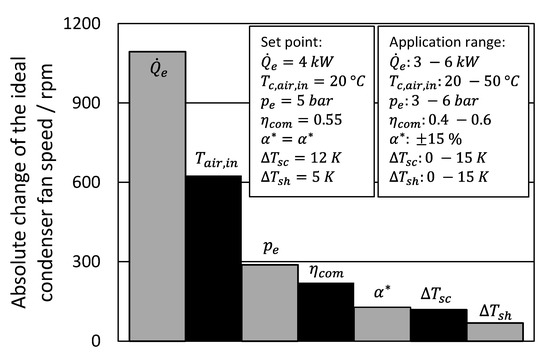
Figure 14.
The absolute change of the ideal condenser fan speed for a given application range and a referring set-point. The results are based on the validated model approach. The influence of the refrigeration capacity () and the ambient temperature () are dominant, followed by the evaporating pressure () and the compressor efficiency ().
In terms of the hybrid model approach, the distribution in Figure 14 clearly explains the reason for the high prediction accuracy of the ideal condenser fan speed at constant input parameters, since the coolant load and ambient temperature are constant within a constant set-point and the suction pressure is coupled by the secondary side of the evaporator with only slight changes. Moreover, the remaining input parameters barely affect the ideal fan speed and vary only within a small range under real application conditions. Despite the exact values only being valid for the VCS under consideration at the reference point, the distribution in Figure 14 does not significantly change for different references and point to the likelihood that the relative order of magnitude may be generalized to other air-cooled VCS with similar characteristics.
In sum, the analysis of the impact of different input parameters on the ideal condenser fan speed reveals high effect of the refrigeration capacity and ambient temperature, moderate impact of the evaporating pressure and compressor efficiency, while the lumped heat transfer coefficient of condenser, subcooling, and superheating have minor impacts. These results are not particularly surprising given the fact that the condensing pressure is the most decisive value for the condenser fan speed optimization. Nevertheless, these findings clarify that only parameters having a high impact on the condensing pressure need to be considered for the ideal condenser fan speed prediction. As a result, an evaporator model is not required and the compressor efficiency, subcooling, and superheating can be kept constant, resulting in a simple, high precision model and a directly solvable system of equations. Hence, an explanation is provided for the high accuracy of the ideal condenser fan speed prediction, although some rough assumptions are made, and only limited plant specifications are required.
5.2. Control Strategy and Energy Saving Potential
The proposed optimization method can be employed to control the condenser fan speed of air-cooled vapor compression systems. Therefore, a control strategy with two separated control loops is suggested and depicted in Figure 15. The first loop adjusts the compressor speed to obtain the required refrigeration capacity and the second loop controls the condenser fan speed according to the model approach. Therefore, uncertainties of the model predictions only have an influence on the fan speed (and on the COSP), but not on the refrigeration capacity. During operation, the described input parameters of the model (Figure 4) must be partially measured (refrigeration capacity, air inlet temperature and evaporating pressure), partially estimated (subcooling and superheating), and the rest is taken from component specifications and physical properties. However, for the optimization within a set-point, all inputs are assumed to be constant.
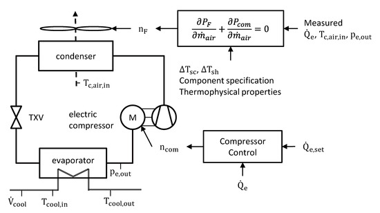
Figure 15.
Control strategy for the set-point optimization of a VCS, based on the proposed model to calculate the ideal condenser fan speed. Required measuring spots are marked.
The proposed control strategy in Figure 15 is applied to the VCS described in Section 2.1 and obtains an energy efficiency loss below 1.5% compared to the ideal operation for all fifteen set-points. The results are highlighted in Figure 16 and outline small deviations for all considered conditions.
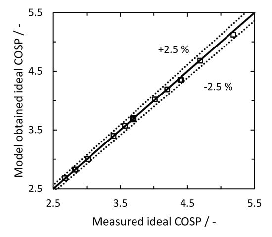
Figure 16.
Experimental validation of the ideal COSP based on the calculated ideal fan speed and the measured ideal COSP for fifteen different constant operation conditions.
As a drawback, there is no guarantee that the exact, ideal operation is reached. However, the investigation in Section 5.1 indicates the prediction accuracy to be quite robust. Consequently, the hybrid model is sufficient to be used in optimization control strategies and due to the simplicity of the model it is expected that it can be used for real time applications. Especially for applications with a quasi-stationary coolant demand, the proposed method represents a promising alternative to extremum seeking control or other advanced methods that may be more accurate but have a high convergence time. Furthermore, the method can be easily adapted to other air-cooled vapor compression systems for optimization purposes and only limited input parameters are necessary. In fact, the required input parameters are usually known during the development process of VCS. Besides real time application, the calculation method can be further used to determine the ideal condensing pressure and ideal fan speed to adjust the parameters of the control method proposed by Chan and Yu et al. [6], for example.
6. Conclusions
In this research study, a steady-state model approach is presented to predict the ideal condenser fan speed of air-cooled vapor compression systems (VCS) within constant operation conditions. The model consists of a hybrid characterization of the main components and the optimization problem is formulated as minimizing the total energy consumption by adjusting the condenser fan and compressor speed. Thereby, the hybrid model approach provides a new optimization method for the calculation of the ideal fan speed, while only limited plant specifications are required. The result is a simple and fast operating optimization method that does not rely on algorithms as compared to other strategies in the literature. To demonstrate the feasibility, a detailed model validation is carried out of 250 steady-state measuring points based on fifteen different operating conditions. The validation reveals a prediction error of the coefficient of system performance (COSP) within ±10%. Moreover, the prediction error of the ideal condenser fan speed is negligible with regard to the flat optimum. An explanation for this high accuracy is given by the discussion of the model assumptions, which implies that only parameters with a high influence on the condensing pressure must be considered for the ideal condenser fan speed calculation. Thereby, the analysis confirms the high effect of refrigeration capacity and ambient temperature reported in the literature. However, the results further suggest that the ideal condenser fan speed can be calculated with sufficient precision, assuming constant evaporating pressure, compressor efficiency, subcooling, and superheating, respectively. In addition, a set-point optimization control strategy is proposed on the basis of the model approach and obtains the maximal efficiency of the VCS for the fifteen different set-points. Consequently, the hybrid model is suitable to be utilized in optimization control strategies, and is expected to be used in real time applications due to the simplicity of the model. Furthermore, the method can be easily adapted to other air-cooled VCS for optimization purposes. Therefore, the results provide a deep insight into the set-point optimization and hybrid steady-state modeling of air-cooled vapor compression systems.
Author Contributions
S.A. outlined the structure and content of this article. S.A. performed the validation and investigation. C.K. proved the content. S.A. wrote the manuscript. All authors have read and agreed to the published version of the manuscript.
Funding
This research received no external funding.
Acknowledgments
We acknowledge support for the Article Processing Charge from the Open Access Publication Fund of the Technische Universität Ilmenau.
Conflicts of Interest
The authors declare no conflict of interest.
Nomenclature
| Area/m2 | |
| Speed of sound/m/s | |
| Mean specific heat capacity/J/(kg∙K) | |
| Specific enthalpy/J/kg | |
| Current/A | |
| Overall heat transfer coefficient/W/(m2∙K) | |
| Refrigerant mass flow rate/kg/s | |
| Rotation speed/rpm | |
| Power/W | |
| Pressure/bar | |
| Heat flux/W | |
| Evaporating enthalpy/J/kg | |
| Specific gas constant/J/(kg∙K) | |
| Coefficient of determination/% | |
| Temperature/°C | |
| Voltage/V | |
| Specific volume m3/kg | |
| Volume flow rate/m3/s | |
| Vapor fraction | |
| Real gas factor/- | |
| Greek Letters | |
| Convective heat transfer coefficient/W/(m2∙K) | |
| Compressor efficiency/- | |
| Substitution | |
| Density/kg/m3 | |
| Heat exchanger characteristic/- | |
| Subscripts | |
| Air | |
| Condenser | |
| Compressor | |
| Coolant | |
| Evaporator | |
| Fan | |
| Isentropic | |
| Ideal | |
| Inlet | |
| Outlet | |
| Refrigerant | |
| Subcooling | |
| Superheating | |
| Abbreviations | |
| Coefficient of Performance/- | |
| Coefficient of System Performance/- | |
| Magnetic inductive flow meter | |
| Number of Transfer Units | |
| Polyalkylene glycol | |
| Root mean square error | |
| 1,1,1,2-Tetrafluorethan | |
| Thermostatic expansion valve | |
| Vapor compression cycle | |
| Vapor compression system | |
Appendix A

Figure A1.
Instrumented air-cooled VCS. 1: Compressor, 2: Condenser (covered), 3: TXV and Evaporator (covered), 4: Fan (covered), 5: Coriolis sensor, 6: Sound velocity sensor, 7: Air inlet, 8: Air outlet, 9: Coolant inlet, 10: Coolant outlet.
Figure A1.
Instrumented air-cooled VCS. 1: Compressor, 2: Condenser (covered), 3: TXV and Evaporator (covered), 4: Fan (covered), 5: Coriolis sensor, 6: Sound velocity sensor, 7: Air inlet, 8: Air outlet, 9: Coolant inlet, 10: Coolant outlet.

Table A1.
Mahle GmbH serial battery cooling unit component description.
Table A1.
Mahle GmbH serial battery cooling unit component description.
| Component | Description | Specification |
|---|---|---|
| Evaporator | Serial component of MAHLE Behr GmbH & Co. KG refrigerant-coolant evaporator (Chiller) | Plate heat exchanger Plate amount: 50 Fluid guidance: Refrigerant “S-Flow”, Coolant “I-Flow” |
| Compressor | Suction gas-cooled electric scroll | Displacement: 24 cm3 Speed: 2400–6000 rpm |
| Condenser | Serial component of MAHLE Behr GmbH & Co. KG air-refrigerant condenser Fin tube type cross-flow system | Four passes with 15, 10, 6 und 4 tubes in1st, 2nd, 3rd and 4th pass respectively Receiver between 3rd and 4th pass |
| Expansion valve | Thermostatic expansion valve of Otto Egelhof GmbH & Co. KG. | Capacity: 2 ton Charge: C6 |
| Fan | Serial component of Spal Automotive | Diameter: 305 mm Speed: 800 to 4000 rpm. |
| Refrigerant-Oil | Serial component of Sanden Inc. Product name: SP-A2 | Polyalkylene glycol (PAG) synthetic oil |
Table A2.
Sensor description.
Table A2.
Sensor description.
| Sensor | Manufacturer | Product Name |
|---|---|---|
| Data logger | Dewetron GmbH | System: DEWE2-M Cards: 2402-dSTG, 2402dACC, CNT, 2402-V, EPAD2-TH8, EPAD2-RTD8 |
| Thermocouple–refrigerant | Electornic Sensor GmbH | IKT 15/10/2KSTS33/2m/ZEH/MFM.K |
| Thermocouple–coolant | Electornic Sensor GmbH | EST 01 |
| Pt100–coolant | SONTEC Sensorbau GmbH | TP1051-A0B1C3D1, TE6-G1/2-A0B1C4D2 |
| Pt100–air | Electornic Sensor GmbH | PT100A 20/050/NB/4 Cu TT17/2 m/LR12.S30 |
| Current | Deweton GmbH | CLAMP-DC-POWER-4-EXT with PA-IT-65-S-BUNDLE, PA-IT-205-S-BUNDLE |
| Fan speed | Keyence Deutschland GmbH | FS-N40 |
| Compressor speed | Brüel Kjaer GmbH | Type 4524 |
| Sound velocity | Anton Paar Germany GmbH | L-SONIC 6100 with PICO 3000 |
| Pressure | ALTHEN GmbH | PDCR 5060-TB-A2-CC H0-PC-030B0000G |
| Coriolis sensor | Emersson | Micro Motion ELITE Coriolis Messsystem: CMF025M176N4FZGZZZMC with Micro Motion 2700 Messumformer: 2700R12CFZGZZZ |
| MID | Siemens AG | MAG 5100 TW with MAG 6000 IP 67 |
Table A3.
Measurement uncertainty of the instruments of the measuring chain MR: regarding measurement range, No declaration: regarding measurement value.
Table A3.
Measurement uncertainty of the instruments of the measuring chain MR: regarding measurement range, No declaration: regarding measurement value.
| Element | Measuring Chain | Uncertainty | Distribution |
|---|---|---|---|
| Pt100 | Sensor | 0.05 °C | normal |
| - | Module | 0.08 °C | rectangular |
| Thermocouple | Sensor | 0.5 °C | normal |
| - | Module | 0.2 °C | rectangular |
| Pressure | Sensor | 0.3% | normal |
| - | Module, Input | 0.02%, 0.02% MR | rectangular |
| - | Module, Output | 0.03% | rectangular |
| Coriolis | Sensor | 0.1% | normal |
| - | Module, Input | 0.02%, 0.02% MR | rectangular |
| - | Module, Output | 0.05% | rectangular |
| MID | System | 0.15% | normal |
| Sound Velocity | Sensor | 0.1 m/s | normal |
| - | Transducer | 0.12% | rectangular |
| - | Module, Input | 0.02%, 0.02% MR | rectangular |
| - | Module, Output | 0.05% | rectangular |
| - | Calculation | 0.96% | normal |
| Acceleration (Compressor speed) | System | 1% | normal |
| Fiber optic (Fan speed) | System | 0.1% | normal |
| Current (Compressor) | Sensor | 83 ppm | rectangular |
| - | Module | 0.02%, 0.02% MR | rectangular |
| Voltage (Compressor) | Sensor | 83 ppm | rectangular |
| - | Module | 0.3%, 0.02% MR | rectangular |
| Current (Fan) | Sensor | 270 ppm | rectangular |
| - | Module | 0.02%, 0.02% MR | rectangular |
| Voltage (Fan) | Sensor | 270 ppm | rectangular |
| - | Module | 0.3%, 0.02% MR | rectangular |
Appendix B
The validation of the refrigerant property models of Equations (11) and (12) is shown in Figure A2. The error of the property model is within 3%. The coefficient of determination for the specific volume and the condensing pressures are 99.99% and 99.85%, respectively. Constant entropy of 1730 J/kgK is assumed for the calculation of the specific volume. For a significant change in entropy, the value must be adjusted. However, for the research in this paper, no change of is necessary.

Figure A2.
Validation of specific volume model approach (a). Validation of condensing pressure model approach (b).
Figure A2.
Validation of specific volume model approach (a). Validation of condensing pressure model approach (b).

The validation of the model is presented for the working fluid R134a and the property data are taken from Span and Wagner [35]. For the same pressure boundaries, the working fluids R1234yf and R290 (Propane) have a maximal error of 6% and 3% for specific volume, and 3% and 3.5% for condensing pressure prediction, respectively.
Appendix C
The coupling function of the air mass flow rate and the refrigerant mass flow rate is given as
with the substitution
and
and
The derivation of the refrigerant mass flow rate to the air mass flow rate is given as:
with
Both gradients of Equation (A5) can be developed separately:
and
The combination of the Equations (A7) and (A8) leads to:
Inserting the substitutions from Equation (A4) leads to the derivation of the coupling function:
Appendix D
The coefficient of determination in percent is defined as
the root mean square error is defined as
the relative root mean square error in percent is defined as
where is the number of validation test data, and indicate the predicted and the measured value of one test point , respectively.
References
- EIA. Residential Energy Consumption Survey. U.S. Energy Information Administration 2015. Available online: https://www.eia.gov/consumption/residential/index.php (accessed on 30 September 2020).
- Tiat, S.; Keung, J. Green Building Design Guide. S. Building & Construction Authority, Singapore 2015. Available online: https://www.bca.gov.sg/GreenMark/others/3rd_Green_Building_Masterplan.pdf (accessed on 30 September 2020).
- UN-Enviorment. The Importance of Energy Efficiency in the Refrigeration, Air-conditioning and Heat Pump Sectors 2018. Available online: https://ozone.unep.org/sites/default/files/2019-08/briefingnote-a_importance-of-energy-efficiency-in-the-refrigeration-air-conditioning-and-heat-pump-sectors.pdf (accessed on 30 September 2020).
- Jensen, J.B.; Skogestad, S. Optimal operation of simple refrigeration cycles. Comput. Chem. Eng. 2007, 31, 712–721. [Google Scholar] [CrossRef]
- Jakobsen, A.; Rasmussen, B. Energy-optimal speed control of fans and compressors in a refrigeration system. In Proceedings of the Eurotherm 62, Grenoble, France, 17–18 November 1998; pp. 317–323. [Google Scholar]
- Chan, K.; Yu, F. Optimum Setpoint of Condensing Temperature for Air-Cooled Chillers. HVAC&R Res. 2004, 10, 113–127. [Google Scholar]
- Larsen, L. Model Based Control of Refrigeration Systems. Ph.D. Thesis, Aalborg University, Aalborg, Denmark, 2005. Available online: https://www.osti.gov/etdeweb/servlets/purl/20833740 (accessed on 30 September 2020).
- Yu, F.; Chan, K. Tune up of the set point of condensing temperature for more energy efficient air cooled chillers. Energy Convers. Manag. 2006, 47, 2499–2514. [Google Scholar] [CrossRef]
- Wan, H.; Cao, T.; Hwang, Y.; Oh, S. A review of recent advancements of variable refrigerant flow air-conditioning systems. Appl. Therm. Eng. 2020, 169, 114893. [Google Scholar] [CrossRef]
- Zhao, L.; Cai, W.-J.; Ding, X.-D.; Chang, W.-C.; Chang, V.W.-C. Decentralized optimization for vapor compression refrigeration cycle. Appl. Therm. Eng. 2013, 51, 753–763. [Google Scholar] [CrossRef]
- Qiao, H.; Radermacher, R.; Aute, V. A Review for Numerical Simulation of Vapor Compression Systems. In Proceedings of the International Refrigeration and Air Conditioning Conference, Purdue University, West Lafayette, IN, USA, 12–15 July 2010; pp. 1–10. Available online: https://docs.lib.purdue.edu/cgi/viewcontent.cgi?article=2089&context=iracc (accessed on 30 September 2020).
- Zhang, G.; Xiao, H.; Zhang, P.; Wang, B.; Li, X.; Shi, W.; Cao, Y. Review on recent developments of variable refrigerant flow systems since 2015. Energy Build. 2019, 198, 444–466. [Google Scholar] [CrossRef]
- Scarpa, M.; Emmi, G.; De Carli, M. Validation of a numerical model aimed at the estimation of performance of vapor compression based heat pumps. Energy Build. 2012, 47, 411–420. [Google Scholar] [CrossRef]
- Zhao, L.; Cai, W.; Ding, X.; Chang, W. Model-based optimization for vapor compression refrigeration cycle. Energy 2013, 55, 392–402. [Google Scholar] [CrossRef]
- Jakobsen, A.; Rasmussen, B.D.; Skovrupity, M.J.; Fredsted, J. Development of Energy Optimal Capacity Controlin Refrigeration Systems. In Proceedings of the 8th International Refrigeration Conference, Purdue University, West Lafayette, IN, USA, 25–28 July 2000; pp. 329–336. Available online: https://docs.lib.purdue.edu/cgi/viewcontent.cgi?article=1498&context=iracc (accessed on 30 September 2020).
- Braun, M.; Walton, P.; Beck, S. Illustrating the relationship between the coefficient of performance and the coefficient of system performance by means of an R404 supermarket refrigeration system. Int. J. Refrig. 2016, 70, 225–234. [Google Scholar] [CrossRef]
- Ruiz, A.G.; Garrido, J.; Vázquez, F.; Morilla, F. A hybrid modeling approach for steady-state optimal operation of vapor compression refrigeration cycles. Appl. Therm. Eng. 2017, 120, 74–87. [Google Scholar] [CrossRef]
- Yang, J.; Chan, K.; Dai, T.; Yu, F.; Chen, L. Hybrid Artificial Neural Network−Genetic Algorithm Technique for Condensing Temperature Control of Air-Cooled Chillers. Procedia Eng. 2015, 121, 706–713. [Google Scholar] [CrossRef]
- Yu, F.; Ho, W.; Chan, K.; Sit, R. Logistic regression-based optimal control for air-cooled chiller. Int. J. Refrig. 2018, 85, 200–212. [Google Scholar] [CrossRef]
- Shin, J.-H.; Kim, Y.-I.; Cho, Y.-H. Development of Operating Method of Multi-Geothermal Heat Pump Systems Using Variable Water Flow Rate Control and a COP Prediction Model Based on ANN. Energies 2019, 12, 3894. [Google Scholar] [CrossRef]
- Goyal, A.; Staedter, M.A.; Garimella, S. A review of control methodologies for vapor compression and absorption heat pumps. Int. J. Refrig. 2019, 97, 1–20. [Google Scholar] [CrossRef]
- Behrooz, F.; Mariun, N.; Marhaban, M.; Radzi, M.; Ramli, A. Review of Control Techniques for HVAC Systems—Nonlinearity Approaches Based on Fuzzy Cognitive Maps. Energies 2018, 11, 495. [Google Scholar] [CrossRef]
- Yu, F.; Ho, W. Load allocation improvement for chiller system in an institutional building using logistic regression. Energy Build. 2019, 201, 10–18. [Google Scholar] [CrossRef]
- Larsen, L.F.S.; Thybo, C.; Stoustrup, J.; Rasmussen, H. A method for online steady state energy minimization, with application to refrigeration systems. In Proceedings of the 43rd IEEE Conference on Decision and Control (CDC), Nassau, Bahamas, 14–17 December 2004; Volume 5, pp. 4708–4713. [Google Scholar]
- Ding, X.; Cai, W.; Jia, L.; Wen, C.; Zhang, G. A hybrid condenser model for real-time applications in performance monitoring, control and optimization. Energy Convers. Manag. 2009, 50, 1513–1521. [Google Scholar] [CrossRef]
- Huang, Y.; Khajepour, A.; Ding, H.; Bagheri, F.; Bahrami, M. An energy-saving set-point optimizer with a sliding mode controller for automotive air-conditioning/refrigeration systems. Appl. Energy 2017, 188, 576–585. [Google Scholar] [CrossRef]
- Yeh, T.-J.; Chen, Y.-J.; Hwang, W.-Y.; Lin, J.-L. Incorporating fan control into air-conditioning systems to improve energy efficiency and transient response. Appl. Therm. Eng. 2009, 29, 1955–1964. [Google Scholar] [CrossRef]
- Jain, N.; Alleyne, A.G. Exergy-based optimal control of a vapor compression system. Energy Convers. Manag. 2015, 92, 353–365. [Google Scholar] [CrossRef]
- Burns, D.; Bortoff, S.; Laughman, C.; Guay, M. Comparing Realtime Energy-Optimizing Controllers for Heat Pumps. In Proceedings of the 17th International Refrigeration and Air Conditioning Conference, Purdue University, West Lafayette, IN, USA, 9–12 July 2018; Available online: https://docs.lib.purdue.edu/cgi/viewcontent.cgi?article=3007&context=iracc (accessed on 30 September 2020).
- Wang, W.; Li, Y. Real-time optimization of intermediate temperature for a cascade heat pump via extreme seeking. In Proceedings of the 13th International Modelica Conference, Regensburg, Germany, 4–6 March 2019; pp. 251–258. [Google Scholar]
- Bejarano, G.; Alfaya, J.A.; Ortega, M.G.; Vargas, M. On the difficulty of globally optimally controlling refrigeration systems. Appl. Therm. Eng. 2017, 111, 1143–1157. [Google Scholar] [CrossRef]
- He, X.; Liu, S.; Asada, H. Modeling of vapor compression cycles for advanced controls in HVAC systems. In Proceedings of the 1995 American Control Conference—ACC’95, Seattle, WA, USA, 21–23 June 1995; pp. 3664–3668. [Google Scholar]
- Hipp, C.; Schauer, M.; Zimmermann, R. System for Controlling the Temperature of an Electric Energy Storage Device. Patent Nr. WO 2019/016021 A2, 2019. Available online: https://patentimages.storage.googleapis.com/77/97/f2/7be732563f0615/WO2019016021A2.pdf (accessed on 28 September 2020).
- Youbi-Idrissi, M.; Bonjour, J.; Terrier, M.-F.; Marvillet, C.; Meunier, F. Oil presence in an evaporator: Experimental validation of a refrigerant/oil mixture enthalpy calculation model. Int. J. Refrig. 2004, 27, 215–224. [Google Scholar] [CrossRef]
- Span, R.; Wagner, W. Equations of State for Technical Applications. I. Simultaneously Optimized Functional Forms for Nonpolar and Polar Fluids. Int. J. Thermophys. 2003, 24, 1–39. [Google Scholar] [CrossRef]
- Heide, R. Stoffdatenbestimmung des Gemisches Kältemittel R134a-Öl ND8; Institut für Luft- und Kältetechnik Gemeinnützige Gesellschaft mbH: Dresden, Germany, 1998; Available online: https://www.ilkdresden.de/en/ (accessed on 28 September 2020).
- Jean-Marc, L.; Louis, V.; Evelyne, M.; Lottin, O. Oil Concentration Measurement in Saturated Liquid Refrigerant Flowing Inside a Refrigeration Machine. Int. J. Thermodyn. 2001, 4, 53–60. [Google Scholar]
- Braumoeller, J.; Riedel, R.; Schenk, J. Messung der Schallgeschwindigkeit in R134a-Oel-Gemischen; Institut für Luft- und Kältetechnik gemeinnützige Gesellschaft mbH: Dresden, Germany, 2004; Available online: https://www.ilkdresden.de/en/ (accessed on 28 September 2020).
- JCGM, Evaluation of measurement data—Guide to the expression of uncertainty in measurement. Joint Committee for Guides in Metrology 2008. Available online: https://www.bipm.org/en/publications/guides/gum.html (accessed on 28 September 2020).
- Angermeier, S.; Föhner, L.; Kerler, B.; Karcher, C. Uncertainty in measurement of a vapor compression system. In Proceedings of the 27th Fachtagung für Experimentelle Strömungsmechanik, Erlangen, Germany, 3–5 September 2019; Available online: https://www.gala-ev.org/images/Beitraege/Beitraege2019/pdf/46.pdf (accessed on 28 September 2020).
- Žukauskas, A. Heat transfer from tubes in crossflow. Adv. Heat Transf. 1972, 8, 93–160. [Google Scholar]
- Chi, J.; Didion, D. A simulation model of the transient performance of a heat pump. Int. J. Refrig. 1982, 5, 176–184. [Google Scholar] [CrossRef]


Publisher’s Note: MDPI stays neutral with regard to jurisdictional claims in published maps and institutional affiliations. |
© 2020 by the authors. Licensee MDPI, Basel, Switzerland. This article is an open access article distributed under the terms and conditions of the Creative Commons Attribution (CC BY) license (http://creativecommons.org/licenses/by/4.0/).