Abstract
Optimizing the operation of ground source heat pumps requires simulation of both short-term and long-term response of the borehole heat exchanger. However, the current physical and neural network based models are not suited to handle the large range of time scales, especially for large borehole fields. In this study, we present a hybrid model for long-term simulation of BHE with high resolution in time. The model uses an analytical model with low time resolution to guide an artificial neural network model with high time resolution. We trained, tuned, and tested the hybrid model using measured data from a ground source heat pump in real operation. The performance of the hybrid model is compared with an analytical model, a calibrated analytical model, and three different types of neural network models. The hybrid model has a relative RMSE of 6% for the testing period compared to 22%, 14%, and 12% respectively for the analytical model, the calibrated analytical model, and the best of the three investigated neural network models. The hybrid model also has a reasonable computational time and was also found to be robust with regard to the model parameters used by the analytical model.
1. Introduction
Ground source heat pumps (GSHPs) use the heat capacity of the ground to provide efficient heating and cooling for buildings. GSHP is widely recognized as an essential technology for the future of energy systems, due to its high efficiency and ability to store energy. In 2015, GSHPs provided 90.9 TWh of energy worldwide, which grew at 10.3% per year from 2010 to 2015 [1]. Sweden is one of the pioneers in GSHP, where around 20% of the heating for the residential and service sector comes from GSHPs. In recent years, the GSHP market in Sweden has shifted from small GSHP for single-family houses to large GSHPs and borehole thermal energy storage (BTES) for commercial and institutional buildings, often used in combination with other heat sources [2]. This trend is expected to continue since an increasing proportion of renewable energy in the energy mix has focused the need of integrating thermal storage in district energy systems [3].
The heat demand of a building does not constrain the operation of GSHPs that work in combination with other heat sources. This provides flexibility to the heating systems that can be utilized to heat a building with reduced economic and environmental costs by optimizing the operation of the heating system. Models are necessary for optimizing the operation of a GSHP. Optimal operation of GSHP requires the short-term response of the borehole heat exchanger (BHE) [4], and the long-term response of the BHE to ensure that the performance of the GSHP does not deteriorate over its lifetime [5]. Therefore, a long-term model with high time resolution is required to optimize the operation of a BHE. The considerable variation in timescales makes the modeling of BHE particularly challenging.
Modeling of BHE is an active research field. The models developed can be classified into long-term models and short-term models. Long-term models focus on modeling the ground surrounding the borehole and simplify the heat transfer inside the borehole. Hence, they cannot accurately represent the short-term response of the borehole [6]. Short-term models have a more detailed representation of the borehole, but do not consider the interaction between boreholes, which affects the long-term performance of the borehole [7].
Several numerical models for long-term performance of BHE, based on the finite difference method [8] and the finite element method [9,10] have been presented. The numerical models are used in commercial software [11,12] since they represent the BHE more accurately than analytical models. However, due to high computational time, the numerical models are seldom used directly, but through pre-calculated non-dimensional response functions, called g-functions. Therefore, the numerical models can only be used for a limited number of BHE configurations. Analytical models are less restricted in terms of BHE configuration and hence are preferred in many cases.
Most long-term analytical models represent the boreholes as finite line sources (FLSs). This solution, first proposed by Eskilson [8], was later used by Zeng et al. [13]. Since then, several researchers have improved the FLS model. The improvements have reduced the computational time [14,15,16] made the representation of the BHE more accurate [7], included a more detailed representation of the ground [17,18] and made it possible to represent different BHE configurations [19,20,21,22].
The recent advances in BHE modeling have made the models more accurate, but the complexity of the solutions has also increased, which reduces their usefulness to many professionals [23]. The increased complexity not only makes the models harder for implementing but also increases the computational time. Moreover, for simulations less than a few hours, the long-term models need to be coupled with short-term models.
Several studies have used both numerical [24,25,26] and analytical approaches for short-time models. Similar to the long-term models, the short-term numerical models can be more precise than the analytical models, but they have higher computational cost, and they are difficult to couple with dynamic simulations [27]. A common analytical approach for the short-term models is to represent the borehole as a network of resistors and capacitors [27,28,29,30,31]. Javed and Claesson [32] also represented the borehole as a thermal network but in the Laplace domain. Other analytical models simplify the problem by defining the borehole pipes as an infinite line source [33], or as a single pipe of an equivalent radius [34,35,36,37].
Despite the advances, there are still many issues in modeling of BHE. One of the issues is the modeling of groundwater-filled boreholes [38,39] which are common in Scandinavia. The coupling of long-term models with short-term models is a challenge [5,24,40] and the computational time required for simulation of such models makes them unfeasible for optimizing the operation of large GSHPs. Moreover, the accuracy of detailed models depends on the accuracy of a large number of parameters. However, the uncertainty of the parameters is high, especially the ground parameters [41]. Determining accurate properties of the ground is an active research field [42] and obtaining accurate properties of the ground in an economically feasible way is still a significant challenge.
Artificial neural networks (ANNs) are often used as a solution for such complex problems. ANN models are data-driven models with a structure that vaguely mirrors the function of a brain. An ANN consists of a network of interconnected nodes, as shown in Figure 1. Each node consists of a summation function that calculates the weighted sum of outputs of the previous layer of nodes and an activation function that introduces non-linearity into the ANN model. The weights of the ANN are calculated using the training data. ANNs are capable of approximating any continuous function [43]. Due to their ability to detect complex non-linear relationships between the inputs and outputs, ANNs are used to solve several complex problems. The use of ANN in heating, ventilation, and air-conditioning systems has also increased in the last two decades [44].
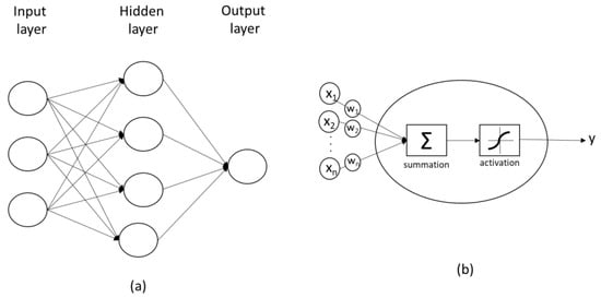
Figure 1.
Schematic of (a) an ANN and (b) a single neuron.
Several studies have used ANN as a solution to the difficulties in the modeling of BHE and obtaining the parameters. ANN leverages the increase in data available in recent years, due to better monitoring of GSHP to solve the issues of BHE modeling. Esen and Inalli [45], Sun et al. [46], and Fannou et al. [47] used ANN to predict the overall performance of the GSHP. ANN has also been used for design [48,49], determination of ground properties [50], and g-function generation [23,51].
Gang and Wang [52] and Lee et al. [53] developed ANN models of BHE as a component, for control of GSHP. Both studies developed ANN models to predict the outlet temperature of a BHE, and both studies used numerical models of a single borehole to train the model. Gang and Wang [52] used fluid inlet temperature and temperatures outside the wall of the pipes and temperature outside the wall of the grouting as inputs. Lee et al. [53] used the heat load of the borehole and outlet temperature of the previous step as input. Both studies concluded that using information from the previous time steps improves the accuracy of the model. The ANN models considered in these studies are not suitable for long-term simulation as both the models were trained using data from short simulations, 9–10 weeks. Moreover, the numerical models used to train the ANN only considered a limited domain around the borehole, and the interaction between the boreholes was not considered.
ANNs were used in the above examples since they did not have many of the issues of the classical modeling techniques of BHE. ANN models have a computational time of less than a second on a standard computer [53]. ANN models use the training data to calculate the weights of the models; hence they do not require any parameters that might be hard to obtain. The ANN models can deduce the complex relationships between the inputs and outputs. These relationships are otherwise hard to determine due to natural convection in the borehole, groundwater flow, heterogeneous ground, etc. However, for the ANN model to predict the outputs accurately, it is necessary to choose the right set of inputs and have a large set of data covering the entire range of operation of the BHE. Due to the large heat capacity of the ground, the thermal response of BHE is influenced by the entire thermal history of the BHE. Therefore, for any BHE model to have an accurate long-term prediction, it must consider the entire thermal history of the BHE. Selecting the input set for such an ANN will be challenging. Moreover, obtaining a training set covering the full range of operations is very difficult, since the thermal history changes with time, especially for an unbalanced system.
In this paper, we propose a hybrid approach that uses a simple long-term analytical model with low time resolution to guide the ANN model as a solution to this issue. This approach attempts to combine the analytical model’s long-term modeling capability with ANN models’ high accuracy and simplicity.
2. GSHP Installation
The proposed BHE model is applied to a GSHP installation at a hospital in Umeå, Sweden. The GSHP is designed to provide 95% of the cooling load of the hospital and 5% of the heating load. The remaining heating and cooling loads are supplied by the district heating and cooling network and additional heat pumps. The GSHP consists of 125 boreholes, three heat pumps, and a heat exchanger for domestic hot water production, as shown in Figure 2. The boreholes are divided into two groups, A and B, which have independent fluid loops.
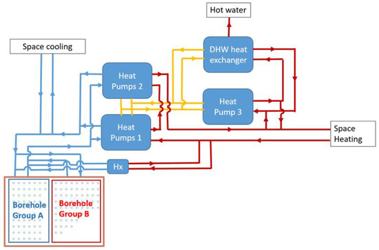
Figure 2.
Schematic of the GSHP (Reproduced from [54], Infroma UK Limited: 2020).
The GSHP provides both heating and cooling throughout the year. The operation of the heat pump is governed by the cooling demand during summer and by heating demand during winter. The GSHP has three operation modes, heat production and free cooling mode, active cooling and free cooling mode, and active cooling mode. During winter, when the heating demand governs the heat pumps, the GSHP operates in heat production and free cooling mode. In this mode, the heat required by the evaporators of the heat pumps 1 and 2 is higher than the cooling demand. Hence, the heat extracted from the BHE provides additional heat. During summer, the cooling load controls the heat pump. On most summer days, the GSHP operates in active cooling and free cooling mode. In active cooling and free cooling mode, free cooling from borehole group B and cooling from heat pumps 1 and 2 supplies the cooling demand. The heat produced by heat pumps 1 and 2 will be greater than space heating demand. Hence, the excess heat from the heat pumps is injected into borehole group A. When borehole group A cannot absorb all the excess heat from the heat pumps, both borehole groups A and B are used for the injection of excess heat. This mode is the active cooling mode. Heat pump 3 uses the intercooler from heat pumps 1 and 2 as a source. It provides heat for domestic hot water and additional heat for space heating during winter.
The borehole groups A and B consists of 62 and 63 boreholes, respectively, as shown in Figure 2. The depth of boreholes in borehole groups A and B are 250 m and 200 m, respectively. The distance between the boreholes is 7 m. The boreholes are single U-tube heat exchangers and are naturally filled with groundwater. The groundwater level is 10 m. The working fluid of the BHE is 20% bioethanol, with heat capacity 4390 J(kg·K)−1 and density 976.6 kg·m−3. The properties of the ground were assumed homogenous. The borehole resistance, thermal conductivity, and undisturbed temperature of the ground and were determined by thermal response test (TRT), while the volumetric heat capacity was obtained from the geological data. Table 1 contains a summary of the properties of the BHE. In Puttige et al. [54], a more detailed description of the properties of the BHE.

Table 1.
Properties of the BHE.
2.1. Measurements
The GSHP has been thoroughly monitored since it started operating in February 2016. Temperature sensors measured the inlet and outlet temperature of each borehole group. The flow rate of each borehole group was measured from March 2017. The flow rate from February 2016 to March 2017 is estimated using the power consumed by the variable speed circulation pump of each borehole group. The tolerance of the temperature sensors are 0.15 °C and the tolerance of the flow meter is 0.33%. The time resolution of the temperature sensors and flow meter are 10 min and 1 min, respectively. However, the monitoring system calculates and stores the hourly average values, the raw data of higher time resolution is deleted at regular intervals. The tolerance of the hourly averaged measurements will be smaller as averaging reduces the random errors.
The hourly averaged measurements from 16 February 2016 to 15 July 2020, 1612 days, is used in this study. For 6.4% of this period, the measurements are not available due to faults in the monitoring system or maintenance. The majority of the missing loads occurs during 2016. 27.9% of data is missing during the first year, while only 1.1% of data is missing for the remaining period. The ground heat loads for the periods without measured data are estimated using the ambient temperature. Figure 3 shows the measured load of borehole groups A and B. The figure shows that the first year contains the most periods without measured data. Figure 3 also shows that the heat injected into the ground during the cooling season is greater than heat extracted from the ground, i.e., the BHE is not balanced.
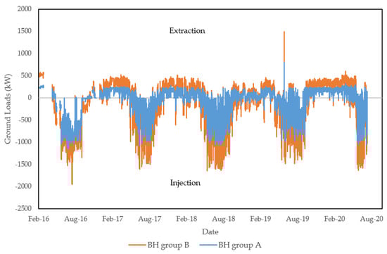
Figure 3.
Measured loads of the BHE.
2.2. Filtering of Data
Figure 3 shows that the measured data have a high variance, where some points have sudden changes in the load. The large differences could be due to a sudden change in the operation mode of the GSHP or due to erroneous measurements. The models are trained to minimize the squared error. Hence, a few points with high errors will disproportionately influence the model. Due to the large number of data points, random measurement errors will not affect the model. However, errors due to malfunctions in the measurement systems will result in some obviously erroneous measurements. These erroneous measurements can be identified as outliers in measured data.
In order to identify the outliers we studied the deviation between the measured data and a prediction model. An analytical model was used to identify the outliers, since the analytical model is not trained on the measured data. Therefore, it is better suited than the hybrid model presented in this study to identify measurement errors. The analytical model developed by Puttige et al. [54] with one-hour time resolution was used. Section 3 includes a short explanation of the model. Figure 4 shows a histogram of the deviation between the load from the analytical model and the measured data. The mean residual for borehole groups A and B are −0.6 kW and 18.5 kW, and the standard deviations of the residuals are 80.4 kW and 57.2 kW for borehole group A and B, respectively. The data points with residuals outside the window of three times the standard deviation are considered as outliers. Note that the deviation includes both measurement errors and model inaccuracies therefore a large window was chosen to accommodate for the inaccuracies of the analytical model. A total of 1.3% of the points were identified as outliers. The outliers were removed from the data, and the filtered data will be used in the following sections.
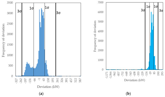
Figure 4.
Histogram of deviation between analytical and measured loads for BH group A (a) and B (b).
3. Hybrid Approach
We present a hybrid ANN model that predicts long-term high time resolution performance of a BHE using the outputs of an analytical model as an input to the ANN model. The hybrid model predicts the hourly load at time t using the inlet temperature and mass flow rate of the last 24 h and the output of the analytical model with 24 h time resolution. With the analytical model to guide the ANN model, the ANN model can predict the long-term performance of the BHE with high accuracy. We chose a simple analytical model that uses only a few physical parameters that are easy to obtain. The authors have presented the analytical model for the BHE described in Section 2 in a previous study [54]. A 24 h time resolution was selected for the analytical model to have a reasonable computational time. Increasing the time resolution of the analytical model improves the accuracy of the hybrid model. An initial trial showed that increasing the time resolution from 30-days to 24 h decreases the relative error of the model by 2.7%, but increasing the time resolution further to one-hour reduces the relative error by just 0.8%. Therefore, we chose a time resolution of 24 h for the analytical model as a tradeoff between computational time and accuracy.
The analytical model uses an approach proposed by Lamarche [20]. The main reason to select this approach was to represent BHE with multiple inputs and outputs. Although the model does not consider geothermal gradient and groundwater, it was chosen because of its simplicity. Moreover, geothermal gradient and groundwater flow were not significant at the installation location [54]. The model’s inputs are inlet temperatures and mass flow rates for each borehole group as inputs, and its outputs are the temperature at the borehole wall and heat load of each borehole. The borehole wall refers to the interface between the ground and the groundwater inside the borehole. The model uses the properties of the ground and the geometric properties of the BHE as parameters. The parameters are listed in Table 1 of Section 2. The model first calculates the coefficients that depend only on the geometry of the BHE. The calculation of these coefficients is a computationally-intensive process, but they are calculated just once for the given geometry and can be used with different inputs and ground parameters. The model uses these coefficients to determine the current temperature at the borehole wall of each borehole using the current inputs and the effect of the previous inputs. The current loads are then calculated using the borehole wall temperatures. Although the borehole wall temperatures and heat loads for each borehole are available, we will only use the average values for each borehole group in this study. For a detailed explanation about the model and its implementation, the readers can refer to [54].
The inputs of the ANN model are chosen to include information about the entire thermal history of the BHE. Hence, the selected inputs for the ANN model are the inlet temperature and mass flow rate of the last 24 h and the output of the last step of the analytical model before time t. The outputs of the analytical model are calculated using the inlet temperature and mass flow rate of all time until the last step. Since the analytical model has a time resolution of 24 h, the last time step of the analytical model can end 1 to 24 h before the time t. Hence, the number of hours between the end of the last step of the analytical and the current time is included as an additional input.
Several studies have used the result that the thermal history of a few immediate hours is more important than the thermal history of the past to decrease computational time by aggregating loads of the past thermal history [24,55,56]. The studies show that past loads can be aggregated into larger time steps without affecting the accuracy of the model. We used the same approach to reduce the number of inputs to the ANN model. Reducing the number of inputs reduces the complexity of the ANN model, which not only reduces the computational time but also reduces the possibility of overtraining. Therefore, instead of using hourly steps as the input for the last 24 h, we used six hourly steps and an aggregated step of 18 h for the remainder of the 24 h.
Thus, the inputs to the ANN model are:
- Prediction step: inlet temperature (Tin,A,t, Tin,B,t) and mass flow (mfA,t, mfB,t) of both borehole group;
- Thermal history of 24 hours: Inlet temperature and mass flow rate of 6 hourly steps (Tin,A,t-1, mfA,t-1, Tin,B,t-1, mfB,t-1, Tin,A,t-2, mfA,t-2, Tin,B,t-2, mfB,t-2, Tin,A,t-6, mfA,t-6, Tin,B,t-6, mfB,t-6,), and one 18 h aggregated step (Tin,A,18h, mfA,18h, Tin,B,18h, mfB,18h) for both borehole group;
- The output of the last step of the analytical model before time t: Borehole wall temperature (Tb,A,ana, Tb,B,ana) and heat load (PA,ana, PB,ana) of both borehole group;
- Number of hours after the last step of the analytical model (Naa);
The outputs of the ANN model are:
- Prediction step: Heat load of both borehole groups (PA,t, PB,t)
Figure 5 shows all the inputs and outputs of the ANN model on a timeline.
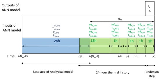
Figure 5.
Inputs and outputs of the ANN model represented on a timeline.
The total number of inputs to the ANN is 37, 4 from the current step, 6 × 4 from 6 previous hourly steps, 4 from the 18 h aggregated step, 4 from the outputs of the analytical model, and Naa. The two outputs of the ANN model are heat loads of the current time step for each borehole group. The choice of the number of hidden nodes was made based on the rule of thumb mentioned in [57], two-thirds of the number of inputs plus the number of outputs. Therefore, the initial architecture was chosen as one hidden layer with 27 nodes. The activation function of the hidden layer is the hyperbolic tangent, and the output layer has a linear activation function. The ANN was implemented in MATLAB (R2020a, The MathWorks Inc, Natick, MA, USA).
The filtered measured data from the GSHP described in Section 2.1 is used for training and testing of the ANN. The data from 2016 is less reliable than the remaining period, as a large portion of the data is missing. Hence the data from 2016 is not used for training or testing of the models. However, the loads during this period will affect the future operation of the BHE. Therefore, the analytical model includes data from 2016. Two years of data, 2017 and 2018, are used for training. The data from 2019 are used as a validation set. The error of the validation set after each training iteration is used to determine the criteria to stop the training algorithm and to select hyper-parameters in Section 4.1. The rest of the data, 2020, is used as a testing set.
The network was trained using the Levenberg-Marquardt (LM) algorithm to minimize the mean squared error (MSE). The probability of overtraining the ANN was reduced using the early stopping criteria. The early stopping criteria stop the optimization algorithm if the MSE of the validation set does not decrease for a specified number of iterations of the algorithm. The LM algorithm only finds local minima and might not find a good solution. Therefore the ANN was trained multiple times, 50 times, with different random initial weights, and the network with the least MSE for the validation set was selected.
4. Results and Discussion
The RMSE of the ANN model for training, validation, and testing are 12.0 kW, 19.3 kW, and 26.6 kW, respectively. The RMSEs correspond to 3.2%, 6.1%, and 7.3% error for training, validation, and training. Note that the percentage of error is with respect to the mean absolute load of the corresponding period. The total error corresponds to 4.9%. The relative RMSE is higher for validation and testing periods compared to training period since the model over fits to the training data to some degree.
Due to a large number of data points, the 30-day moving relative RMSE of the hybrid model is plotted in Figure 6, instead of hourly RMSE. The maximum 30-day moving relative RMSE is 12.3%. The relative RMSE for validation and testing is greater than training but the relative RMSE of in the validation and testing periods is similar. The relative RMSE in the testing period has an upward trend. However, the variation is within the error range of the validation period. To check if the relative RMSE increases in the testing period, we used the data from only 2017 training, and 2018 was used for validation, and 2019 and 2020 were used for testing. Figure 7 shows the moving relative RMSE for this case. For the 19 months of the testing period in Figure 7, the relative RMSE shows no clear increase over time. This implies that the model can be used for predicting the load for multiple years. The relative RMSE for validation and testing is higher in Figure 7 compared to Figure 6. Therefore, we will use the original scheme, with 2017 and 2018 for training, 2019 for validation, and 2020 for testing in this study.
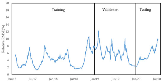
Figure 6.
30-day moving relative RMSE of the hybrid model.
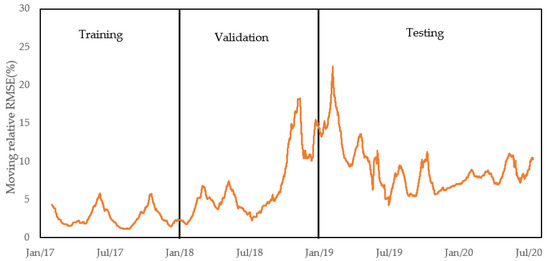
Figure 7.
30-day moving relative RMSE for the hybrid model with one year of training period.
4.1. Model Improvement
The performance of the model was improved by tuning the hyper-parameters of the model and by using an ensemble of multiple neural networks instead of a single network.
4.1.1. Ensemble
Neural network ensemble is a technique to refine the neural network models by using multiple neural networks to solve a problem. In this technique, several ANNs are trained, and then the output of all the networks produce a better prediction than any individual network. Hansen and Salamon [58] first showed that neural network ensembles could be an effective method to reduce the error of ANNs. Since then, several approaches to training individual networks have been developed [59]. In this study, we will use the simple approach of training each of the networks using the same set of data with different initial weights. More complex approaches were not explored since it is outside the scope of our study. The output of the ensemble is calculated as the average of the networks, giving equal weight to each network.
Fifty ANNs were trained using the filtered data set similar to the previous model, but instead of using the predations of the best network, the average of all the networks is used as output. Figure 8 shows the relative RMSE of the average of first N networks. The ensemble of all 50 networks has a relative RMSE of 2.6%, 5.9%, and 6.6% for training, validation, and testing, respectively. Therefore, the average prediction of all the models is better than the prediction of the best model. However, from Figure 8, we notice that after a certain point adding more models does not result in any significant change in the accuracy of the ensemble. Hence the number of models in the ensemble can be lower than 50. The validation relative RMSE changes by less than 0.1% when the number of models varies from 15 to 50. Therefore, an ensemble of 15 models will be used for the remainder of this study. The relative RMSE for training, validation, and testing of the ensemble of 15 models is 2.7%, 5.9%, and 6.7%, respectively.
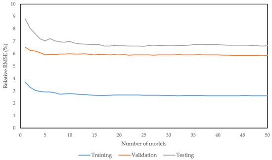
Figure 8.
Variation of the percentage of relative RMSE with the number of models in the ensemble.
4.1.2. Choosing the Number of Hidden Nodes
The number of nodes in the hidden layer is an important parameter of the ANN model. If the number of nodes is too low, the model will be under-fitted, and the model will not be able to represent the variance of the system. If the number of nodes is too high, the model has a higher risk of over-fitted, and random errors of the model will be represented in the model. Therefore, we tried different numbers of hidden nodes to find an appropriate architecture for the ANN.
Table 2 shows the relative RMSE for training, validation, and testing of the model with different numbers of nodes in the hidden layer. Each model is an ensemble of 15 models trained on filtered data. As expected, the training error decreases as the number of nodes increases. The validation error initially decreases as the number of nodes increases. However, increasing the number of nodes after a certain point increases the validation error, i.e., the model overfits the training data after a certain point. The validation error increases when the number of nodes is higher than 45. We, therefore, limit the number of nodes in the hidden to be 45. The number of nodes was not refined further because the difference in the RMSE among the models was not significant, i.e., the choice of the number of nodes would be affected by the random initial weights of the model.
Table 2.
Relative RMSE as a function of the number of nodes in the hidden layer.
4.1.3. Choosing Optimization Algorithm
The choice of the optimization algorithm used for training the network can also have an impact on the accuracy of the model. Hence, we tested three optimization algorithms, namely, scaled conjugate gradient (SCG), Levenberg–Marquardt (LM), and Bayesian regularization within the LM algorithm (BR). The BR algorithm does not use the validation set; therefore, a predefined goal for MSE is set as the stopping criteria for the algorithm. After a few trials, the goal for the MSE was set as 50 kW2.
Table 3 shows the relative RMSE for training, validation, and testing for models trained using the three algorithms. An ensemble of 15 models with 45 nodes in the hidden layer was used, i.e., the parameters selected in the Section 4.1.1 and Section 4.1.2. The SCG algorithm performs significantly worse than the other two algorithms. Both LM and BR have similar RMSE values, but the validation RMSE of the LM model is lower. We, therefore, chose the LM optimization algorithm. Both algorithms use the LM algorithm to update the weights, the BR algorithm uses regularization to reduce overfitting. In the LM model, overfitting was prevented by using early fitting. The results show that LM using early stopping is slightly better than BR and is therefore we chose the LM algorithm.
Table 3.
Relative RMSE of the model for different optimization algorithms
4.1.4. Choosing the Number of Non-Aggregated Steps
In the initial model, we divided the 24 h thermal history into six non-aggregated 1 h steps and one aggregated 18 h step. Increasing the number of non-aggregated steps will increase the number of inputs of the model. A higher number of inputs means more information, which can result in a more accurate model, but the risk of overfitting and local minima is also higher.
Table 4 shows the relative RMSE of the training, validation, and training set. The models use the parameters selected in the Section 4.1.1 and Section 4.1.3. The RMSE of the validation set decreases when the number of non-aggregated steps increases from 3 to 6, but a further increase in the number of non-aggregated steps did not decrease the RMSE of the validation set. We selected the number of non-aggregated steps as six since an additional increase in the number of non-aggregated steps did not improve the model, but the computational time for training increased.
Table 4.
Relative RMSE as a function of the number of non-aggregated steps.
4.2. Comparison with Other Models
We evaluated the proposed hybrid model by comparing it with various analytical and ANN models for BHE. The models in the following section use the filtered data set described in Section 2.2 for training and testing.
4.2.1. Analytical Models
We compared the hybrid model with the two analytical models presented in [54], ANA, and ANA_calib. ANA is the same model used by the hybrid model but with a time resolution of one hour. ANA_calib is the ANA model, but the properties of the ground calibrated using the measured data. Four parameters are calibrated, namely thermal conductivity of the ground (k), volumetric heat capacity of the ground (ρCp), thermal resistance between the fluid and the borehole wall (Rb), and undisturbed temperature of the ground (Tug). Puttige et al. [54] recommended the used of different parameters for heating and cooling seasons. Based on this recommendation, the loads were determined using two sets of parameters. We used filtered data from 2017 and 2018 to calibrate the model, which is the same dataset as training set of the hybrid model. Table 5 lists the calibrated model parameters for heating and cooling seasons.
Table 5.
Calibrated model parameters.
Figure 9 shows the moving relative RMSE for the two analytical models and the final hybrid model. The hybrid model has lower relative RMSE during the whole period. The ANA_calib and hybrid models use data from 2017 and 2018 for training, and the hybrid model is validated using the data from 2019. None of the models uses the data from 2020. It is therefore best to compare the models by the error of 2020. The relative RMSE for 2020 for ANA, ANA_calib, and hybrid models is 21.9%, 13.2%, and 6.3%. The results show that the error of the hybrid model is significantly lower than the analytical models.
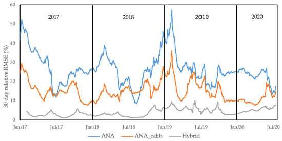
Figure 9.
30-day relative RMSE of the hybrid model compared to two analytical models.
The hybrid model has an advantage in terms of computational time as well. The two analytical models have a computational time of approx. 5 h for each run on a computer with a 3.4 GHz quad-core processor and 16 GB RAM. While the hybrid model has a computational time of approx. 15 min for the analytical model and less than a second for the ANN model. The computational time for calibrating the ANA_calib model is approx. 40 h, while the time for training the hybrid model is approx. 25 min. Note that the computational times for the analytical models do not include the time required for calculating the geometric coefficients, since they were calculated just once for the BHE and used for all the models.
The physical parameters necessary for both the ANA and hybrid models are the geometry of the BHE and four properties of the ground. ANA_calib model uses the measured data to calculate the properties of the ground, so it only requires the geometry of the BHE. However, the accuracy of the parameters required for the hybrid model is lower than regular ANA model since the hybrid model is capable of correcting the inaccuracy of the analytical model. We tested this by adding random error in the range of ±20% to the measured ground parameters, i.e., the measured parameters were multiplied by a random number in the range of 0.8 to 1.2. Two hybrid models with different random errors were tested. The relative RMSE of the models were 6.2% and 6.4% for the testing period.
4.2.2. Neural Network Models
We compared the hybrid model with three different types of neural network models. The first is a simple feedforward network, while the other two networks that use the outputs from the previous time steps.
The inputs of the feedforward network (ANN) are similar to the hybrid model but without the outputs of the analytical model and Naa. Therefore, the inputs of the ANN model are the inlet temperatures and mass flow rates of the current one-hour step, six previous one-hour steps, and one aggregated step of 18 h. The ANN model has 32 inputs. The outputs of the ANN model are the same as the hybrid model, the predicted load of the current step. The suitable number of hidden nodes in the ANN model is determined to be 32, using the same method as Section 4.1.2. An ensemble of 15 ANN models trained using the LM algorithm is used to obtain the predicted loads.
Temporal dependencies of a neural network can be included using a class of neural networks called recursive neural networks (RNN). RNNs use the outputs of previous time steps as inputs of the current time step. Since each step of the RNN depends on the previous step/s, the output of the current step depends on the entire sequence of inputs before the current step, as shown in Figure 10. Therefore, RNNs are capable of considering the history of the BHE. Kose and Petlenkov [60] used RNNs to model BHE, but the structure of the RNN used is not clear. Lee et al. [53] predicted the current outlet temperature using different inputs and found that using the four inputs, current heat load, outlet temperature at the previous time step, heat load at the previous time step, and the outlet temperature at two time steps prior, was the best option. However, they did not use an RNN, but the outlet temperature from the target outputs. In practice, when predicting outlet temperatures of multiple time steps ahead, the target output will not be available. Hence, we must use the simulated output. In this study, we will use inputs similar to [53], but we will use simulated outputs from the previous steps instead of target outputs. The inputs to the RNN model are inlet temperatures and mass flow rate of the current and the previous step for each borehole, and the output of the two previous time steps. The output of the model is the heat loads of borehole groups A and B.
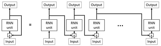
Figure 10.
Schematic of an RNN.
Since the output of the RNN model depends on the sequence of inputs, the inputs must contain the complete time series, i.e., from the start of the operation to the current step. However, the input data has some missing data. To resolve this issue, we calculated the loads during the missing periods using the ambient temperature. The mass flow rate of the BHE group was assumed to be constant and equal to the average mass flow rate of the borehole group during the missing periods. The inlet temperature was calculated using the analytical model with load and mass flow rates as inputs. This method gives us an estimate of the inputs to the RNN model, but these inputs are not accurate. Therefore, we used weighted MSE to calculate the error only when the inputs to the model are reliable. In order to have the same inputs as the hybrid model, the weights were set to 0 for 2016, during periods of missing data, and the points removed by the filtering process described in Section 2.2. The model uses data from 2017 and 2018 as the training set, 2019 as the validation set, and 2020 as the testing set.
An ensemble of 15 models was used to determine the output similar to the hybrid model. The models were trained using, but the early stopping criteria cannot be used for RNN in MATLAB; therefore, the stopping criteria was set by defining the maximum number of iterations. The maximum number of iterations and the number of hidden nodes in the hidden layer were selected by trial and error. We selected 30 as the maximum number of iterations and 5 as the number of hidden nodes.
Typical RNNs like the one described above have an issue called vanishing gradient problem. The vanishing gradient problem causes the long-term inputs to lose their effect on the output, i.e., the output will only depend on the short-term inputs. Hochreiter and Schmidhuber [61] introduced long short-term memory (LSTM) networks as a solution to the vanishing gradient problem. LSTM resolves the issue of vanishing gradients by using gates, sigmoid functions, which decide how much information from the previous steps must be retained, and therefore important information from the previous steps is not lost. In this study, we will use a simpler variant of LSTM introduced by Cho et al. [62] called the gated recursion unit (GRU).
The GRU and the RNN model are similar, with the same training, validation, and testing data sets and the same weights for data and the same inputs and outputs. However, the output of the GRU ht is not used directly as the output of the network. The size of ht (hidden units size) determines how much information is passed from one time step to the next and should not be fixed by the number of outputs of the network. The GRU is therefore implemented using a four-layer network, sequence input layer, GRU layer, fully connected layer, and weighted regression layer. The sequence input layer coverts the input data into the right format so that it can be used in the GRU layer. The GRU layer uses the sequence of inputs to calculate the hidden states. The fully connected layer converts the hidden states into the required output, i.e., the load of the current step. The weighted regression layer calculates the weighted MSE using the measured and simulated loads.
Adam optimizer was used to train the model. The maximum number of iterations set the stopping criteria. The maximum number of iterations, the hidden unit size, and the learning rate of the algorithm were determined by trial and error. The selected number of hidden unit size, the maximum number of iterations, and the learning rate of the algorithm are 50, 250, and 0.02.
Figure 11 shows the moving relative RMSE of the ANN, RNN, GRU, and the final hybrid models. All four models have the same training, validation and testing data. All the models use an ensemble of 15 neural networks. The relative RMSE for the testing set for the hybrid, ANN, RNN, and GRU models is 6.3%, 13.4%, 12.5%, and 13.0%, respectively. The relative RMSE of the hybrid model is about half of the other models. Which shows that the hybrid model is significantly more accurate than the other models.
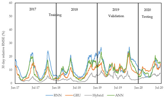
Figure 11.
30-day relative RMSE of the hybrid model compared to three neural network models.
The neural network models do not use the analytical model. Hence, they do not require any geometric parameters of the BHE or the thermal properties of the ground, and they have lower computational times. The run time of the ANN, RNN, and GRU models are 1, 7, and 8 s, respectively, and the training time for the three models is 11, 5, and 90 min. The training and the run time of the hybrid model are 25 and 15 min. The ANN, RNN, and GRU models could be a good option if the required parameters are not available or if the computational time is more important than accuracy for an application.
5. Conclusions
The proposed approach for BHE modeling uses an analytical model with low time resolution to guide an ANN model with high time resolution. This hybrid analytical-ANN model extends the range of typical ANN models, which are limited to short-term simulations, to long-term simulations of BHE, while maintaining good accuracy and reasonable computational time.
The hybrid model was applied to a large GSHP with more than four years of measured data. The measured data was used to train, validate, and test the model. After tuning the parameter of the model, we achieved a relative RMSE of 2.4% for training, 5.6% for validation, and 6.3% for testing. The model has a reasonable computational time of 15 minutes and requires only parameters that are easy to obtain. Moreover, the model is robust with respect to the model parameters used for the supportive analytical model.
The hybrid model was compared with two analytical models and three neural network models. The hybrid model was found to be significantly more accurate than the compared models. The best analytical and neural network models have a relative RMSE of 13.9% and 12.6% for the test set.
Author Contributions
Conceptualization: A.R.P., S.A., R.Ö., and T.O.; Methodology, A.R.P., S.A., R.Ö., and T.O.; Software, A.R.P.; Formal analysis, A.R.P.; Investigation, A.R.P.; Resources, T.O.; Data curation, A.R.P.; Writing—original draft preparation, A.R.P.; Writing—review and editing, A.R.P., S.A., R.Ö., and T.O.; Visualization, A.R.P.; Supervision, S.A., R.Ö., and T.O.; Project administration, T.O.; Funding acquisition, T.O. All authors have read and agreed to the published version of the manuscript.
Funding
This research was funded by Industrial Doctoral School at Umeå University and Umeå Energi AB.
Acknowledgments
We would like to thank Region Västerbotten for providing the field measurements from the heating system at Norrland’s university hospital. We would like to thank Zonghua Gu for his insights and suggestions in developing the neural network models.
Conflicts of Interest
The authors declare no conflict of interest.
Nomenclature
| rb | Borehole radius (m) |
| H | Active borehole depth (m) |
| D | Groundwater level (m) |
| k | Thermal conductivity of the ground (W/(m.K)) |
| ρ | Density (kg/m3) |
| Cp | Specific heat capacity (J/K.kg) |
| Rb | Borehole resistance (m.K/W) |
| T | Temperature (°C) |
| P | Heat load (W) |
| mf | Mass flow rate (kg/s) |
| Naa | Number of hours after the last step of the analytical model |
| Abbreviations | |
| GSP | Ground source heat pumps |
| BTES | Borehole thermal energy storage |
| BHE | Borehole heat exchanger |
| ANN | Artificial neural network |
| TRT | Thermal response test |
| LM | Levenberg–Marquardt |
| MSE | Mean squared error |
| RMSE | Root-mean-squared error |
| SCG | Scaled conjugate gradient |
| BR | Bayesian regularization |
| ANA | Analytical |
| ANA_calib | Calibrated analytical |
| RNN | Recursive neural networks |
| LSTM | Long short-term memory |
| GRU | Gated recursion unit |
| Subscripts | |
| ug | Undisturbed ground |
| b | Borehole wall |
| in | Fluid inlet |
| A | Borehole group A |
| B | Borehole group B |
| t | time |
| 18 h | 18-h time step |
| ana | From analytical model |
References
- Lund, J.W.; Boyd, T.L. Direct utilization of geothermal energy 2015 worldwide review. Geothermics 2016, 60, 66–93. [Google Scholar] [CrossRef]
- Gehlin, S.; Andersson, O. Geothermal energy use, country update for Sweden. In Proceedings of the European Geothermal Congress 2019, Den Haag, The Netherlands, 11–14 June 2019. [Google Scholar]
- Lund, H.; Werner, S.; Wiltshire, R.; Svendsen, S.; Thorsen, J.E.; Hvelplund, F.; Mathiesen, B.V. 4th Generation District Heating (4GDH): Integrating smart thermal grids into future sustainable energy systems. Energy 2014, 68, 1–11. [Google Scholar] [CrossRef]
- Zhang, C.; Wang, Y.; Liu, Y.; Kong, X.; Wang, Q. Computational methods for ground thermal response of multiple borehole heat exchangers: A review. Renew. Energy 2018, 127, 461–473. [Google Scholar] [CrossRef]
- Li, M.; Li, P.; Chan, V.; Lai, A.C.K. Full-scale temperature response function (G-function) for heat transfer by borehole ground heat exchangers (GHEs) from sub-hour to decades. Appl. Energy 2014, 136, 197–205. [Google Scholar] [CrossRef]
- Lamarche, L. Short-term behavior of classical analytic solutions for the design of ground-source heat pumps. Renew. Energy 2013, 57, 171–180. [Google Scholar] [CrossRef]
- Cimmino, M.; Bernier, M. A semi-analytical method to generate g-functions for geothermal bore fields. Int. J. Heat Mass Transf. 2014, 70, 641–650. [Google Scholar] [CrossRef]
- Eskilson, P. Thermal Analysis of Heat Extraction Boreholes; Lund Institute of Technology Sweden, Department of Mathematical Physics: Lund, Sweden, 1987. [Google Scholar]
- Monzó, P.; Puttige, A.R.; Acuña, J.; Mogensen, P.; Cazorla, A.; Rodriguez, J.; Montagud, C.; Cerdeira, F. Numerical modeling of ground thermal response with borehole heat exchangers connected in parallel. Energy Build. 2018, 172. [Google Scholar] [CrossRef]
- Naldi, C.; Zanchini, E. A new numerical method to determine isothermal g-functions of borehole heat exchanger fields. Geothermics 2019, 77, 278–287. [Google Scholar] [CrossRef]
- Hellström, G.; Sanner, B. Software for dimensioning of deep boreholes for heat extraction. Proc. Calorstock 1994, 94, 195–202. [Google Scholar]
- Spitler, J.D. GLHEPRO-A design tool for commercial building ground loop heat exchangers. In Proceedings of the Fourth International Heat Pumps in Cold Climates Conference, Aylmer, PQ, Canada, 17–18 August 2000. [Google Scholar]
- Zeng, H.Y.; Diao, N.R.; Fang, Z.H. A finite line-source model for boreholes in geothermal heat exchangers. Heat Transf. Asian Res. 2002, 31, 558–567. [Google Scholar] [CrossRef]
- Lamarche, L.; Beauchamp, B. A new contribution to the finite line-source model for geothermal boreholes. Energy Build. 2007, 39, 188–198. [Google Scholar] [CrossRef]
- Lamarche, L. A fast algorithm for the hourly simulations of ground-source heat pumps using arbitrary response factors. Renew. Energy 2009, 34, 2252–2258. [Google Scholar] [CrossRef]
- Marcotte, D.; Pasquier, P. Fast fluid and ground temperature computation for geothermal ground-loop heat exchanger systems. Geothermics 2008, 37, 651–665. [Google Scholar] [CrossRef]
- Molina-Giraldo, N.; Blum, P.; Zhu, K.; Bayer, P.; Fang, Z.H. A moving finite line source model to simulate borehole heat exchangers with groundwater advection. Int. J. Therm. Sci. 2011, 50, 2506–2513. [Google Scholar] [CrossRef]
- Abdelaziz, S.L.; Ozudogru, T.Y.; Olgun, C.G.; Martin II, J.R. Multilayer finite line source model for vertical heat exchangers. Geothermics 2014, 51, 406–416. [Google Scholar] [CrossRef]
- Lazzarotto, A. A network-based methodology for the simulation of borehole heat storage systems. Renew. Energy 2014, 62, 265–275. [Google Scholar] [CrossRef]
- Lamarche, L. Mixed arrangement of multiple input-output borehole systems. Appl. Therm. Eng. 2017, 124, 466–476. [Google Scholar] [CrossRef]
- Cimmino, M. A finite line source simulation model for geothermal systems with series- and parallel-connected boreholes and independent fluid loops. J. Build. Perform. Simul. 2018, 11, 414–432. [Google Scholar] [CrossRef]
- Dusseault, B.; Pasquier, P.; Marcotte, D. A block matrix formulation for efficient g-function construction. Renew. Energy 2018, 121, 249–260. [Google Scholar] [CrossRef]
- Dusseault, B.; Pasquier, P. Efficient g-function approximation with artificial neural networks for a varying number of boreholes on a regular or irregular layout. Sci. Technol. Built Environ. 2019, 25, 1023–1035. [Google Scholar] [CrossRef]
- Yavuzturk, C.; Spitler, J.D. A short time step response factor model for vertical ground loop heat exchangers. ASHRAE Trans. 1999, 105, 475–485. [Google Scholar]
- Xu, X.; Spitler, J.D. Modeling of vertical ground loop heat exchangers with variable convective resistance and thermal mass of the fluid. In Proceedings of the 10th International Conference on Thermal Energy Storage Ecostock, Pomona, NJ, USA, 31 May–2 June 2006. [Google Scholar]
- Naldi, C.; Zanchini, E. A one-material cylindrical model to determine short-and long-term fluid-to-ground response factors of single U-tube borehole heat exchangers. Geothermics 2020, 86, 101811. [Google Scholar] [CrossRef]
- Cazorla-Marín, A.; Montagud-Montalvá, C.; Tinti, F.; Corberán, J.M. A novel TRNSYS type of a coaxial borehole heat exchanger for both short and mid term simulations: B2G model. Appl. Therm. Eng. 2020, 164, 114500. [Google Scholar] [CrossRef]
- Zarrella, A.; Scarpa, M.; De Carli, M. Short time step analysis of vertical ground-coupled heat exchangers: The approach of CaRM. Renew. Energy 2011, 36, 2357–2367. [Google Scholar] [CrossRef]
- Bauer, D.; Heidemann, W.; Müller-Steinhagen, H.; Diersch, H.-J.G. Thermal resistance and capacity models for borehole heat exchangers. Int. J. Energy Res. 2011, 35, 312–320. [Google Scholar] [CrossRef]
- Pasquier, P.; Marcotte, D. Short-term simulation of ground heat exchanger with an improved TRCM. Renew. Energy 2012, 46, 92–99. [Google Scholar] [CrossRef]
- De Rosa, M.; Ruiz-Calvo, F.; Corberán, J.M.; Montagud, C.; Tagliafico, L.A. A novel TRNSYS type for short-term borehole heat exchanger simulation: B2G model. Energy Convers. Manag. 2015, 100, 347–357. [Google Scholar] [CrossRef]
- Javed, S.; Claesson, J. New Analytical and Numerical Solutions for the Short-term Analysis of Vertical Ground Heat Exchangers. ASHRAE Trans. 2011, 117, 3–12. [Google Scholar]
- Li, M.; Lai, A.C.K. New temperature response functions (G functions) for pile and borehole ground heat exchangers based on composite-medium line-source theory. Energy 2012, 38, 255–263. [Google Scholar] [CrossRef]
- Wei, J.; Wang, L.; Jia, L.; Zhu, K.; Diao, N. A new analytical model for short-time response of vertical ground heat exchangers using equivalent diameter method. Energy Build. 2016, 119, 13–19. [Google Scholar] [CrossRef]
- Young, T.R. Development, Verification, and Design Analysis of the Borehole Fluid Thermal Mass Model for Approximating Short Term Borehole Thermal Response. Ph.D. Thesis, Oklahoma State University, Stillwater, OK, USA, 2004. [Google Scholar]
- Lamarche, L.; Beauchamp, B. New solutions for the short-time analysis of geothermal vertical boreholes. Int. J. Heat Mass Transf. 2007, 50, 1408–1419. [Google Scholar] [CrossRef]
- Lamarche, L. Short-time analysis of vertical boreholes, new analytic solutions and choice of equivalent radius. Int. J. Heat Mass Transf. 2015, 91, 800–807. [Google Scholar] [CrossRef]
- Spitler, J.D.; Javed, S.; Ramstad, R.K. Natural convection in groundwater-filled boreholes used as ground heat exchangers. Appl. Energy 2016, 164, 352–365. [Google Scholar] [CrossRef]
- Johnsson, J.; Adl-Zarrabi, B. Modelling and evaluation of groundwater filled boreholes subjected to natural convection. Appl. Energy 2019, 253, 113555. [Google Scholar] [CrossRef]
- Ruiz-Calvo, F.; De Rosa, M.; Monzó, P.; Montagud, C.; Corberán, J.M. Coupling short-term (B2G model) and long-term (g-function) models for ground source heat exchanger simulation in TRNSYS. Application in a real installation. Appl. Therm. Eng. 2016, 102, 720–732. [Google Scholar] [CrossRef]
- Witte, H.J.L. Error analysis of thermal response tests. Appl. Energy 2013, 109, 302–311. [Google Scholar] [CrossRef]
- Luo, J.; Rohn, J.; Xiang, W.; Bertermann, D.; Blum, P. A review of ground investigations for ground source heat pump (GSHP) systems. Energy Build. 2016, 117, 160–175. [Google Scholar] [CrossRef]
- Hornik, K.; Stinchcombe, M.; White, H. Multilayer feedforward networks are universal approximators. Neural Netw. 1989, 2, 359–366. [Google Scholar] [CrossRef]
- Mohanraj, M.; Jayaraj, S.; Muraleedharan, C. Applications of artificial neural networks for refrigeration, air-conditioning and heat pump systems—A review. Renew. Sustain. Energy Rev. 2012, 16, 1340–1358. [Google Scholar] [CrossRef]
- Esen, H.; Inalli, M. Modelling of a vertical ground coupled heat pump system by using artificial neural networks. Expert Syst. Appl. 2009, 36, 10229–10238. [Google Scholar] [CrossRef]
- Sun, W.; Hu, P.; Lei, F.; Zhu, N.; Jiang, Z. Case study of performance evaluation of ground source heat pump system based on ANN and ANFIS models. Appl. Therm. Eng. 2015, 87, 586–594. [Google Scholar] [CrossRef]
- Fannou, J.-L.C.; Rousseau, C.; Lamarche, L.; Kajl, S. Modeling of a direct expansion geothermal heat pump using artificial neural networks. Energy Build. 2014, 81, 381–390. [Google Scholar] [CrossRef]
- Chen, S.; Mao, J.; Chen, F.; Hou, P.; Li, Y. Development of ANN model for depth prediction of vertical ground heat exchanger. Int. J. Heat Mass Transf. 2018, 117, 617–626. [Google Scholar] [CrossRef]
- Arat, H.; Arslan, O. Optimization of district heating system aided by geothermal heat pump: A novel multistage with multilevel ANN modelling. Appl. Therm. Eng. 2017, 111, 608–623. [Google Scholar] [CrossRef]
- Zhang, Y.; Zhou, L.; Hu, Z.; Yu, Z.; Hao, S.; Lei, Z.; Xie, Y. Prediction of layered thermal conductivity using artificial neural network in order to have better design of ground source heat pump system. Energies 2018, 11, 1896. [Google Scholar] [CrossRef]
- Pasquier, P.; Zarrella, A.; Labib, R. Application of artificial neural networks to near-instant construction of short-term g-functions. Appl. Therm. Eng. 2018, 143, 910–921. [Google Scholar] [CrossRef]
- Gang, W.; Wang, J. Predictive ANN models of ground heat exchanger for the control of hybrid ground source heat pump systems. Appl. Energy 2013, 112, 1146–1153. [Google Scholar] [CrossRef]
- Lee, D.; Ooka, R.; Ikeda, S.; Choi, W. Artificial neural network prediction models of stratified thermal energy storage system and borehole heat exchanger for model predictive control. Sci. Technol. Built Environ. 2019, 25, 534–548. [Google Scholar] [CrossRef]
- Puttige, A.R.; Andersson, S.; Östin, R.; Olofsson, T. Improvement of borehole heat exchanger model performance by calibration using measured data. J. Build. Perform. Simul. 2020, 13, 430–442. [Google Scholar] [CrossRef]
- Bernier, M.A.; Pinel, P.; Labib, R.; Paillot, R. A multiple load aggregation algorithm for annual hourly simulations of GCHP systems. Hvac&R Res. 2004, 10, 471–487. [Google Scholar]
- Claesson, J.; Javed, S. A load-aggregation method to calculate extraction temperatures of borehole heat exchangers. ASHRAE Trans. 2012, 118, 530–539. [Google Scholar]
- Heaton, J. Introduction to Neural Networks with Java; Heaton Research, Inc.: Chesterfield, MO, USA, 2008; ISBN 1604390085. [Google Scholar]
- Hansen, L.K.; Salamon, P. Neural network ensembles. IEEE Trans. Pattern Anal. Mach. Intell. 1990, 12, 993–1001. [Google Scholar] [CrossRef]
- Zhou, Z.-H.; Wu, J.; Tang, W. Ensembling neural networks: Many could be better than all. Artif. Intell. 2002, 137, 239–263. [Google Scholar] [CrossRef]
- Kose, A.; Petlenkov, E. System identification models and using neural networks for ground source heat pump with ground temperature modeling. In Proceedings of the 2016 International Joint Conference on Neural Networks (IJCNN) IEEE, Vancouver, BC, Canada, 24–29 July 2016; pp. 2850–2855. [Google Scholar]
- Hochreiter, S.; Schmidhuber, J. Long Short-Term Memory. Neural Comput. 1997, 9, 1735–1780. [Google Scholar] [CrossRef] [PubMed]
- Cho, K.; Van Merriënboer, B.; Gulcehre, C.; Bahdanau, D.; Bougares, F.; Schwenk, H.; Bengio, Y. Learning phrase representations using RNN encoder-decoder for statistical machine translation. arXiv 2014, arXiv:1406.1078. [Google Scholar]


Publisher’s Note: MDPI stays neutral with regard to jurisdictional claims in published maps and institutional affiliations. |
© 2020 by the authors. Licensee MDPI, Basel, Switzerland. This article is an open access article distributed under the terms and conditions of the Creative Commons Attribution (CC BY) license (http://creativecommons.org/licenses/by/4.0/).