Analysis of Building Parameter Uncertainty in District Heating for Optimal Control of Network Flexibility

Abstract

Network flexibility is the use of the thermal capacity of water that is contained in the district heating network pipes to store energy and shift the heat load in time. Through optimal control, this network flexibility can aid in applications such as peak shaving and operational heat pump optimisation. Yet, optimal control requires perfect predictions and complete knowledge of the system characteristics. In reality, this is not the case and uncertainties exist. To obtain insight into the importance of these uncertainties, this paper studies the influence of imperfect knowledge of building parameters on the optimal network flexibility activation and its performance. It is found that for the optimisation of heat pump operation, building parameter uncertainties do not present large risks. For peak shaving, a more robust result can be achieved by activating more network flexibility than may be required.

1. Introduction

In order to limit air pollution and green house gas emissions, a fundamental change in our energy system is required. In 2019, heating and cooling in the tertiary and residential sectors were responsible for 41.7% of the total final energy use in the EU28 [1], while 79% of energy used in European households went to space heating (SH) and domestic hot water (DHW) [2]. Furthermore, 75% of the energy used for heating and cooling of buildings is based on fossil fuels, while only 18% originates from renewable and residual energy sources (R²ES) (of which 90% biomass) [3]. Thus, the heating and cooling sector for buildings represents a large fraction of the total energy use and it is a viable opportunity for improving the system efficiency and energy source portfolio.

Energy efficiency for the heating and cooling sector can be improved by district heating and cooling (DHC) systems in areas with a large heat/cold density, i.e., a large heat/cold demand per square kilometre. As Frederiksen and Werner stated, the fundamental idea of district heating (DH) is found in local synergies between the heat sources and demand [4]. By connecting sources and demand through a pipe network, new heat and cold sources can be unlocked, such as combined heat and power (CHP), waste incineration, industrial residual heat, combustible renewables, and geothermal sources, thereby improving the energy efficiency and operational costs of the energy system. Connoly et al. [5] found that the inclusion of DHC in an EU energy efficiency strategy for 2050 can reduce the total costs for the heating and cooling of buildings by 15%.

In order to increase the share of R²ES, their intermittency must be dealt with. One possible solution is to introduce energy flexibility in the energy system. Its definition is as follows [6]: ‘Energy flexibility is the ability to shift the energy injection into or energy extraction from a system in time to bypass system limitations’. By introducing energy flexibility, the integration of R²ES can be improved, e.g., by preventing curtailment of R²ES. In this respect, DHC systems offer an interesting opportunity; they contain multiple thermal energy storage systems (TES), such as water storage tanks, aquifers, borefields, building thermal inertia, and the network itself. Intelligently deploying TES for creating energy flexibility [7] can pave the way to large shares of R²ES.

Within this context, this paper focuses on energy flexibility that is created by the thermal capacity of the water contained in DH network pipes, referred to as network flexibility from now on. By temporarily increasing/decreasing the supply temperature in the DH network, the network is charged/discharged. This way, energy can be stored for a while, bridging the gap between heat generation and heat demand. A detailed description of a typical network flexibility activation can be found in [6].

By solving an optimal control problem (OCP), two applications of network flexibility are considered in this paper. There is operational heat pump optimisation, in which the interaction with the day-ahead market is optimised, and peak shaving, in which the use of an expensive and/or polluting peak unit is minimised [8,9,10]. In the literature, other applications of network flexibility can be found: CHP optimisation [11,12,13], R²ES integration [14,15,16], and providing ancillary services [17].

However, the OCPs that are described in these studies all consider perfect predictions and perfect knowledge of the system model and parameters. However, this is not the case in reality, and the OCP solution will deviate from the actual optimal control strategy. This study investigates the influence of these deviations on the control performance. Before going into the novelty and the specific research questions of this paper, the uncertainties that play a role in DH systems are introduced first, followed by a discussion on robust control of energy systems with uncertainty: how to determine a control strategy that can achieve a satisfactory result in (almost) all possible cases?

1.1. Uncertainties in District Heating Systems

Kim et al. [18] divided uncertainty into three categories. Model uncertainties are caused by a lack of knowledge regarding the physical system and/or the necessity to simplify and neglect certain aspects to keep the model solvable within acceptable time. Process uncertainties either refer to inaccurate actuators and sensors, or to the inability to measure certain system states. Forecast uncertainties relate to the imperfect forecasts that are made of system disturbances, such as weather, electricity prices, R²ES generation, etc.

One example is heat demand uncertainty, which is, in fact, the result of other uncertainties. The main contributors are: user behaviour predictions, weather forecasts, and unknown building construction. Of these, the former two are related to forecasts, while the latter belongs to the model uncertainties category.

In order to accommodate the user behaviour uncertainties, several tools have been set up to stochastically generate user behaviour profiles describing indoor temperature set-points, electrical appliance usage, internal heat gains, and DHW use. These are mostly based on surveys and hence represent the typical behaviour of a certain population. Such tools include StROBe [19], Strathclyde University Demand Profile Generator [20], DELORES [21], and a Japanese activity-based modelling tool [22].

Regarding weather predictions, weather servers that provide regular weather forecasts can often be used to analyse weather uncertainties. For example, by combining imperfect weather forecasts with the corresponding measurements of the weather as it actually occurred, Oldewurtel [23] analysed the influence of these uncertainties for building heating.

The final contribution to heat demand uncertainty is the imperfect knowledge regarding building construction and building energy performance. Especially on the district or city level, building energy performance related data are often unavailable [24,25]. Because of the lack of detailed input data on building level, archetype buildings are often used. Archetype buildings are buildings that are considered to be representative for a larger group of buildings. As an example, the TABULA project defines archetype dwellings, i.e., typical dwellings, for multiple European countries [26]. For Belgium, 30 archetype buildings are characterised in terms of their geometry and U-values for roof, ground floor, exterior wall, and windows. Thanks to the rising popularity and availability of geographical information systems and geospatial data, the building geometry of all individual buildings can be included within district energy simulations. However, thermal quality data of the building envelope are still rarely available, although they are collected in some countries for the calculation and allocation of building energy performance certificates. Unfortunately, these data are often not shared due to privacy issues. To overcome this issue, De Jaeger et al. [27] developed a method for estimating the thermal quality of the building envelope based on construction year and geometrical data of the building based on statistical data from the Flemish energy performance certificates database.

In this paper, only the last source of heat demand uncertainty, the imperfect knowledge of building parameters, is discussed.

1.2. Robust Control of Energy Systems

With these uncertainties, the optimal solution of a deterministic OCP may be far from optimal for the actual system, which leads to a reduced performance. Hence, OCPs have been reformulated in the literature in order to integrate uncertainties and reduce the associated risk. Three approaches can be discerned, which range in complexity.

Firstly, deterministic model predictive control (MPC) is a first step towards improved robustness. In short, an MPC solves an OCP with a receding horizon, i.e., at frequent points in time, the OCP is solved with updated forecasts and system state measurements. The resulting optimal control strategy is then applied to the actual system [28]. Although the embedded OCP still does not consider the uncertainties, the regular update of relevant predictions and states ensures that the MPC control actions can adapt through time, all the while trying to minimise the objective. This technique is applied by Arnold and Göran [29], who alleviated prediction errors of electricity demand and R²ES generation in an electricity system with connected TES systems. They analysed the MPC performance by running Monte-Carlo simulations and concluded that the TES systems provided the MPC with an opportunity to deal with most of the prediction errors, thereby preventing unplanned start-ups of plants.

A second approach uses stochastic modelling in order to determine the robust optimal control of a system. This is done by incorporating probability distributions for the stochastic parameters into the OCP. Different types of stochastic modelling can be found. In single-stage stochastic programming, all control actions are decided at one instance. This is e.g., the case in chance-constrained programming. Here, the chance that a certain constraint will be violated is limited to a certain extent. Bruninx et al. [30] applied such a chance constraint problem in order to ensure that the energy demand in an electricity system would be successfully generated and delivered in e.g., 95% of the cases.

Two-stage optimisation problems are solved in two stages, as explained by Verrilli et al. [31]: ‘In two-stage stochastic programs, the decision variables are divided into two groups: the first-stage variables, which have to be decided before the actual realisation of the uncertain parameters becomes available, and the second stage or recourse variables, which can be decided once the random events occur. These recourse variables are also interpreted as correction actions to compensate any infeasibility from the first-stage decisions’. This technique has been applied multiple times. Wang et al. [32] applied it to the optimal control of a building energy system. In order to test the robust optimal control problem, they compared it to an MPC by running Monte-Carlo simulations of both controllers. They concluded the robust optimal control and the MPC reached about the same performance, but the stochastic OCP could do so with a single evaluation across the whole time horizon. Tian [17] optimised the operation of a CHP that was connected to both the electricity system and a DH system with a two-stage stochastic problem. The goal was to offer ancillary services and participate in the electricity spot market, while the electricity demand is uncertain. Interestingly, network flexibility is applied here in order to increase the CHP profits, yet no DH system uncertainties were included.

Other stochastic programming techniques that are found in the literature include scenario robust optimisation, in which a number of carefully selected scenarios are combined [18] in one OCP. Options to select such scenarios include Sample Average Approximations [31], Monte-Carlo sampling [33], Latin Hypercube Sampling [18], and the point-estimate strategy [34,35]. Monte-Carlo least squares regression analysis [36] and min-max optimisations (worst-case optimisations) have also been applied for the robust control of energy systems [37,38].

Finally, a third approach to reach robust control is by combining the first two: MPC and stochastic optimal control. While Oldewurtel [23] integrated a chance-constrained program for building energy system control into an MPC, Rantzer [39] and Verrilli et al. [31] both developed an MPC that contains a two-stage optimisation problem for DH system control.

This overview shows that plenty of research in the robust control of energy systems has been done. However, to the authors’ knowledge, there has been no research yet in robust control of network flexibility with respect to heat demand uncertainty or any other form of uncertainty in the DH system itself. Hence, the exploratory study that is presented in this paper focusing only on the impact of building parameter uncertainty provides a valuable contribution to the scientific literature.

1.3. Novelty and Research Questions

The main novelty of this paper is the assessment of building parameter uncertainties, leading to an uncertainty on the heat demand magnitude (i.e., the heat demand profile has been scaled up/down with an uncertain time-dependent factor). The term ‘magnitude’ is used in this text to emphasise that there are no timing changes. An example of heat demand profiles that only have magnitude changes is illustrated in Figure 5. The uncertainty on the heat demand magnitude impacts the network flexibility activation in DH systems based on a deterministic OCP. Two applications of network flexibility are studied: (1) operational heat pump optimisation in which the interaction of a central DH heat pump with the day-ahead electricity market is studied and (2) peak shaving.

This study indicates how sensitive the optimal network flexibility activation is to the building parameter uncertainties and, hence, a change in heat demand magnitude, and how much risk is associated with adopting a control strategy based on wrongly estimated building parameters. This paper shows whether simple measures can provide less risk and/or higher profits leading to a more robust control strategy. It is a first step in estimating the importance of robust network flexibility control and to the development of that robust control. The following research questions will be considered:

• How does the optimal network flexibility activation (i.e., the control strategy) alter when the building parameters are different?
• How sensitive is the network flexibility performance to the applied control strategy (and hence to uncertainty)?
• Does this preliminary study lead to insights for a more robust activation of network flexibility?

In this paper, the considered case study is described first. Subsequently, in Section 3, the methodology for the optimal control, the uncertainty on the heat demand and the uncertainty analysis is introduced. Subsequently, the results are presented in Section 4, followed by the discussion in Section 5. Finally, the conclusions are formulated in Section 6.

2. Case Study: GenkNET

The influence of building parameter uncertainty on network flexibility is tested by optimising the control of GenkNET. This is a fictive DH system that is based on the city of Genk, Belgium. To set up this case study, steps 1–4 in Figure 1 were followed. First, the geometrical data from 7775 buildings that were located in Genk were collected from a CityGML LOD2 model. Subsequently, Genk was divided into nine neighbourhoods and for every neighbourhood the average construction year was determined by a Google Streetview scan. In order determine the user behaviour of the people inhabiting these buildings, user behaviour profiles (temperature set-points, internal heat gains, DHW use, etc.) were generated with the stochastic toolbox StROBe [19].

In order to limit the computational complexity of this case study and prevent the simultaneous simulation of 7775 buildings, a thorough aggregation was carried out. Every neighbourhood in GenkNET is now represented by one substation that has to deliver the heat demand of the entire neighbourhood, neglecting the distribution network in a neighbourhood. For more details on this aggregation, please refer to [6]. This leads to the DH system layout that is shown in Figure 2. The nominal supply and return temperatures in this DH system are taken to be 57 ${}^{\circ }\mathrm{C}$ and 37 ${}^{\circ }\mathrm{C}$, respectively. The pipe sizes are determined by the sizing procedure that is presented in [6].

Instead of a whole year analysis, only a limited number of days is tested in this paper. In order to select a representative set of days, two aspects are considered: (1) the overall heat demand, leading to a distinction between winter and transitional (spring and autumn) days. The summer days are not considered, as summer heat demands proved to be too low for interesting network flexibility activations and hence interesting results. (2) The day-ahead electricity price profile can be either stable and positive (small $\Delta p_{\mathrm{e}}$), volatile and positive (large $\Delta p_{\mathrm{e}}$), or become negative during the day (negative $p_{\mathrm{e}}$). The electricity price $p_{\mathrm{e}}$ corresponds to the BELPEX day-ahead market prices in 2014. This leads to a selection of six days, as given in

Table 1. The nine days selected for the GenkNET case. These days will be referred to as <season>_<electricity price>.

Heat Demand	Winter	Trans(itional)
El. Price
Small $\Delta p_{\mathrm{e}}$	16/01	29/03
Large $\Delta p_{\mathrm{e}}$	14/01	17/11
Neg(ative) $p_{\mathrm{e}}$	16/02	16/03

. These days will be referred to as <season>_<electricity price>, according to the names of the columns and rows of Table 1.

In this paper, the heat generation unit is either a central air-to-water heat pump or a base/peak plant combination. The six selected days account for different electricity price profiles that allow for studying different heat pump cases, as the operational heat pump optimisation heavily depends on the electricity price variation through time. In order to study the base/peak plant combination in more depth, different base load ratios are studied. The base load ratio $r_{\mathrm{b}}$ defines the capacity of the base unit ${\dot{Q}}_{\mathrm{b},\max }$ relative to the peak heat demand of the analysed day ${\dot{Q}}_{\mathrm{dem},\max ,\mathrm{day}}$. Three base load ratios are tested: 60%, 80%, and 95%. Note that this will lead to base plant sizes that are different for every case (day and base load ratio).

$$r_{\mathrm{b}}=\frac{{\dot{Q}}_{\mathrm{b},\max }}{{\dot{Q}}_{\mathrm{dem},\max ,\mathrm{day}}}$$

(1)

3. Methodology

This section presents the methodology used. Firstly, it discusses the optimal control problems that will be solved in this study. Secondly, the set-up of the heat demand profiles with uncertainty is presented. Finally, the methodology of the uncertainty analysis in order to assess the influence of the building parameter uncertainty on network flexibility is described.

3.1. Deterministic Optimal Control

In order to determine the optimal network flexibility activation, the toolbox modesto [40] is used. It contains a library of (non-linear) DH component models, including pipe, substation, and heat generation models. The models, as they are used in this study, are presented in Appendix A. These models were specifically developed for determining optimal network flexibility activations, leading to a compromise between computational complexity and accuracy. Hence, these models are suited in order to model the temporary network temperature changes in the DH network and the corresponding energy storage that take place during a network flexibility activation. For more information on the interactions that take place during a network flexibility activation, we refer to [6]. However, note that the models are completely deterministic and they do not take into account any uncertainties.

modesto can automatically assemble the GenkNET DH system optimisation model that is based on its topology and a selection of models and optimisation objective. For each considered case, the network topology remains the same, yet the heat generation site and optimisation objective is changed depending on the studied case. In case of heat pump or peak shaving optimisation, either a heat pump model or a base/peak plant model is included. The optimisation objective depends on the heat generation site, Equations (2) and (3) show the objectives $C_{\mathrm{HP}}$ and $C_{\mathrm{PS}}$ for the operational heat pump and peak shaving optimisation, respectively. In these objectives, $\dot{W}$ is the electrical work done by the heat pump to generate the heat, $p_{\mathrm{e}}\left(i\right)$ is the day-ahead electricity market price during time step i, expressed in €/kWh${}_{\mathrm{el}}$, $\Delta t$ is the time step between two points in time in the discretised OCP with a total of N time steps. ${\dot{Q}}_{\mathrm{b}}$ and ${\dot{Q}}_{\mathrm{p}}$ are the heat delivered by the base and peak plant unit, respectively. Similarly, $p_{\mathrm{b}}$ and $p_{\mathrm{p}}$ are the prices of the heat that is generated by both units. They are expressed in €/kWh${}_{\mathrm{th}}$ and are constant in time. This price already includes the plant energy efficiency. In this study, only the ratio between the two prices is imposed, equal to $p_{\mathrm{p}}/p_{\mathrm{b}}=2$ [41].

$$C_{\mathrm{HP}}=\sum _{\mathrm{i}=1}^N{p}_{\mathrm{e}}\left(i\right){\dot{W}}_{\mathrm{i}}\Delta t$$

(2)

$$C_{\mathrm{PS}}=\sum _{\mathrm{i}=1}^N(p_{\mathrm{b}}{\dot{Q}}_{\mathrm{b},\mathrm{i}}+p_{\mathrm{p}}{\dot{Q}}_{\mathrm{p},\mathrm{i}})\Delta t$$

(3)

The price of heat generation by the base unit is lower than that by a peak unit. Hence, the peak shaving objective causes a preference for the base unit and incentivises peak shaving. The heat pump objective incentivises heat generation on moments during which the electricity price is low. In this study, network flexibility is the only available tool in the OCP for creating energy flexibility. The optimisation is run twice. First, network flexibility is not available, i.e., the supply temperature leaving the plant must remain equal to the nominal value. Second, network flexibility is available, i.e., the supply temperature may change between its nominal value and a value that is 10 ${}^{\circ }\mathrm{C}$ higher. By doing so, the network flexibility activation can be isolated and analysed. The 10 ${}^{\circ }\mathrm{C}$ temperature increase is based on values that are found in literature [42]. A more elaborate explanation on this workflow can be found in [43].

The OCP settings and models are elaborated on in Appendix A.

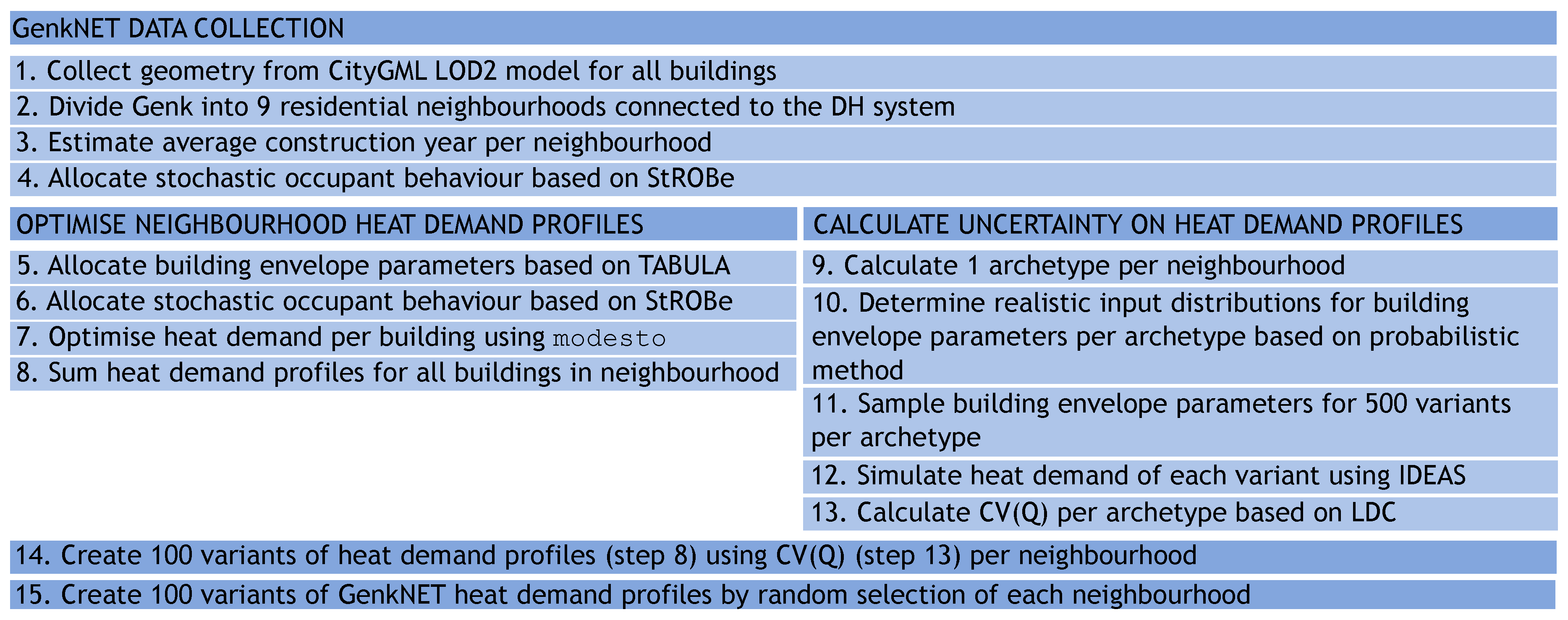
3.2. Heat Demand Profiles

Following the process presented in Figure 1 (steps 5–15), heat demand profiles containing building parameter uncertainties can be set up.

In a first part (steps 5–8), the heat demand profile for every neighbourhood in GenkNET is determined based on a minimum energy use optimisation. Starting from the geometries of the 7775 buildings in Genk (step 1) and the neighbourhood construction year (step 3), building parameters are allocated to each building based on the TABULA archetype U-values [26]. Based on these data and the StROBe user behaviour profiles (step 4), van der Heijde calculated the building heat demand profiles [44], based on the 4th order TEASER RC-model [45]. For this, he used the typical meteorological year of Uccle, Belgium. To calculate the heat demand profiles, van der Heijde made use of modesto in order to determine the heat demand profile that ensures thermal comfort with minimum energy use in every building. Finally, to reach one heat demand profile per aggregated GenkNET neighbourhood, the heat demand profiles of buildings that belong to one neighbourhood are summed.

In a second part (steps 9–13), the uncertainty on the heat demand profiles is calculated. In order to reduce the computational burden, the uncertainty in each neighbourhood is determined through the use of archetype buildings. The archetype building for a neighbourhood is characterised by the estimated average construction year of the neighbourhood (step 3) and the average building geometry. To obtain the average building geometry, the geometry of all buildings is required (step 2). The areas of the façades and roofs are merged towards four orientations (N, E, S, W), with a negligible loss of accuracy [46]. This simplifies calculating the average. This procedure is repeated for every neighbourhood and, resulting in nine archetype buildings.

For these nine archetype buildings, distributions on the U-values of the roof, ground floor, exterior wall, and windows are introduced along with variations on the window-to-wall ratio, based on the method of De Jaeger et al. [27]. The U-values represent the insulation quality of the building envelope and they are defined as the amount of heat transfer through the building component (expressed in W/m${}^2$K). These distributions are estimated to be as realistic as possible when considering the scarcely available data of Genk [27]. Note that building geometry is assumed to be perfectly known, as are user behaviour and weather predictions.

Using these distributions, 500 versions of every archetype building are generated. The distributions of all (9 × 500) generated building parameters can be seen in Figure 3. Next, yearlong simulations of the archetype buildings are carried out in Modelica using the IDEAS model library [47]. These simulations entail a two-zone white-box building envelope model, while the SH system consists of ideal radiator heating. The user behaviour and weather, as they were described in Section 2, are applied. This leads to the distribution in annual SH heat demand in GenkNET shown in Figure 4.

Based on the simulation results, load duration curves (LDC) of every variation are set up and the resulting coefficient of variation (CV) is studied. The CV is equal to the ratio of the standard deviation to the mean of a distribution (i.e., $\sigma /\mu$). The CV for one archetype was found to change in function of the expected SH heat demand of that building ${\dot{Q}}_{\mathrm{arch},\mathrm{SH},\mu }$. In addition, the CV could be well estimated by an exponential in function of the expected SH heat demand of the archetype building, with a, b, and c the fitting parameters that depend on the neighbourhood.

$$\mathrm{CV}({\dot{Q}}_{\mathrm{arch},\mathrm{SH},\mu })=aexp(-b{\dot{Q}}_{\mathrm{arch},\mathrm{SH},\mu })+c$$

(4)

By stating that the archetype building heat demand is the average building heat demand in a neighbourhood with $N_{\mathrm{b}}$ buildings and expected heat demand ${\dot{Q}}_{\mathrm{SH},\mu }$, the following expression for CV can be set up for each neighbourhood:

$$\mathrm{CV}({\dot{Q}}_{\mathrm{SH},\mu })=aexp(-b\frac{{\dot{Q}}_{\mathrm{SH},\mu }}{N_{\mathrm{b}}})+c$$

(5)

In a third part (steps 14–15), the uncertainties (steps 9–13) are added to the optimal heat demand profiles (steps 5–8). Based on the exponential curves that describe the CV, new SH heat demand profiles for each neighbourhood in GenkNET are set up. To do so, a normal distribution is assumed, which has been used in the literature before in order to describe building heat or electricity demand distributions [23,30,33,39,48]. When considering the distribution in Figure 4, this seems a reasonable assumption. This allows the use of the following quantile function:

$$F^{-1}\left(p\right)=\mu +\sigma \sqrt{2}{\mathrm{erf}}^{-1}(2p-1)$$

(6)

For a normally distributed variable, $F^{-1}\left(p\right)$ is the value of the variable for which there is a probability p, such that $F^{-1}\left(p\right)$ is greater than or equal to the variable. In this equation, $\mu$ and $\sigma$ are the expected value and standard deviation of the variable, and ${\mathrm{erf}}^{-1}$ is the inverse error function.

To set up the SH heat demand profile of version v, the following is done. The value for p is randomly selected from a uniform distribution between 0 and 1. Subsequently, starting from the optimal SH heat demand profiles (steps 5–8) [44], at every point in time the quantile function is applied along with the CV that corresponds to the expected heat demand ${\dot{Q}}_{\mathrm{SH},\mu ,\mathrm{i}}$ at the point in time i:

$${\dot{Q}}_{\mathrm{SH},v,\mathrm{i}}\left(p\right)={\dot{Q}}_{\mathrm{SH},\mu ,\mathrm{i}}\left(1+\mathrm{CV}({\dot{Q}}_{\mathrm{SH},\mu ,\mathrm{i}})\sqrt{2}{\mathrm{erf}}^{-1}(2p-1)\right)$$

(7)

This process yields curves that are scaled by a factor changing through time, with the factor depending on the heat demand at that time.

An additional step is added in order to introduce a small amount of random behaviour. Following the autoregressive process AR(1), an extra term was added to the heat demand profile. This term has an autocorrelation of 0.75 between two subsequent points in time separated by 15 min and it has a standard deviation of 3% of ${\dot{Q}}_{\mathrm{SH},\mu ,\mathrm{i}}$, following the prediction error analysis in [49].

This way, 100 different SH heat demand profiles are generated for every neighbourhood. To end up with 100 different versions of GenkNET, one generated profile of every neighbourhood is grouped together. This grouping was done fully at random, although it could be argued that there might be correlations between neighbourhoods, e.g., if the U-values were underestimated in one neighbourhood, the chances are that this also happened in other neighbourhoods. However, this effect is not included here.

No uncertainty was added to the DHW heat demand, so these are simply added to the different SH heat demand profiles. Finally, the left of Figure 5 shows the heat demand of GenkNET of all 100 versions for the Trans_Neg$p_e$ day. The right graph shows 11 selected profiles, spread over the entire range. Note that the range in variation is similar to that shown in Figure 4, with approximately a factor 2 between the most extreme cases. The extra random changes that were added to the profile have little effect and do not change the overall behaviour.

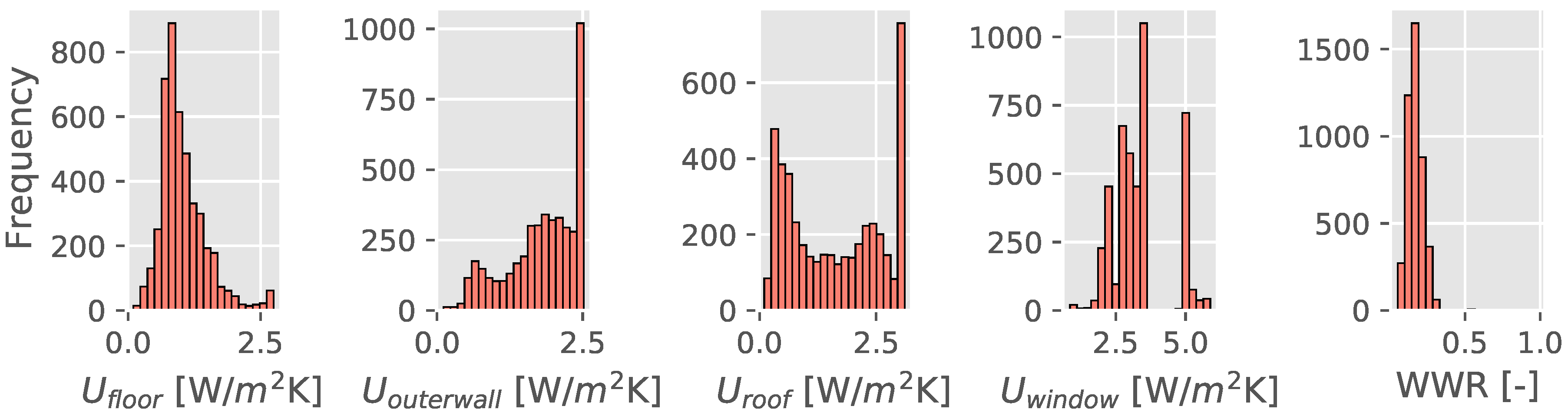
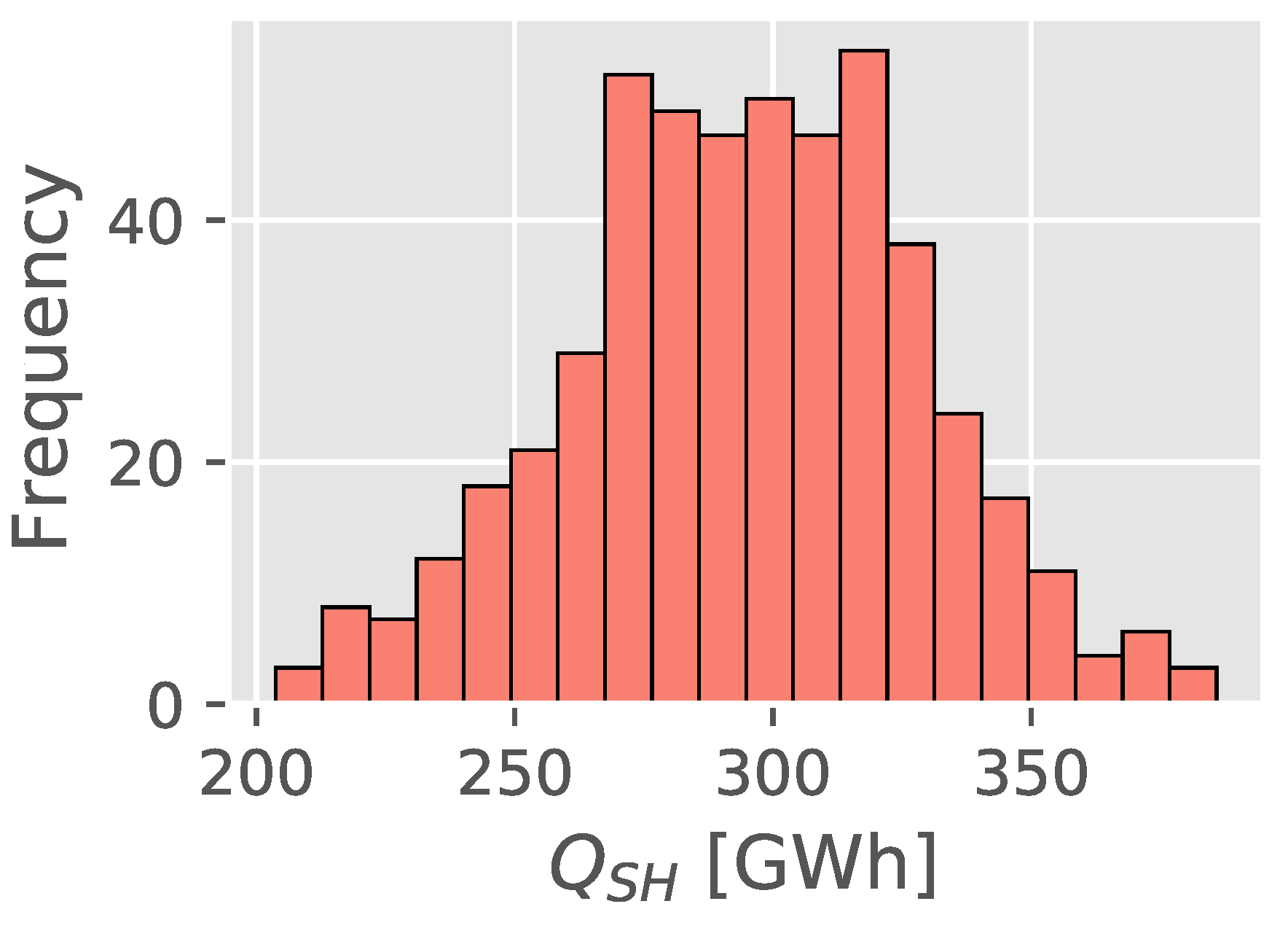
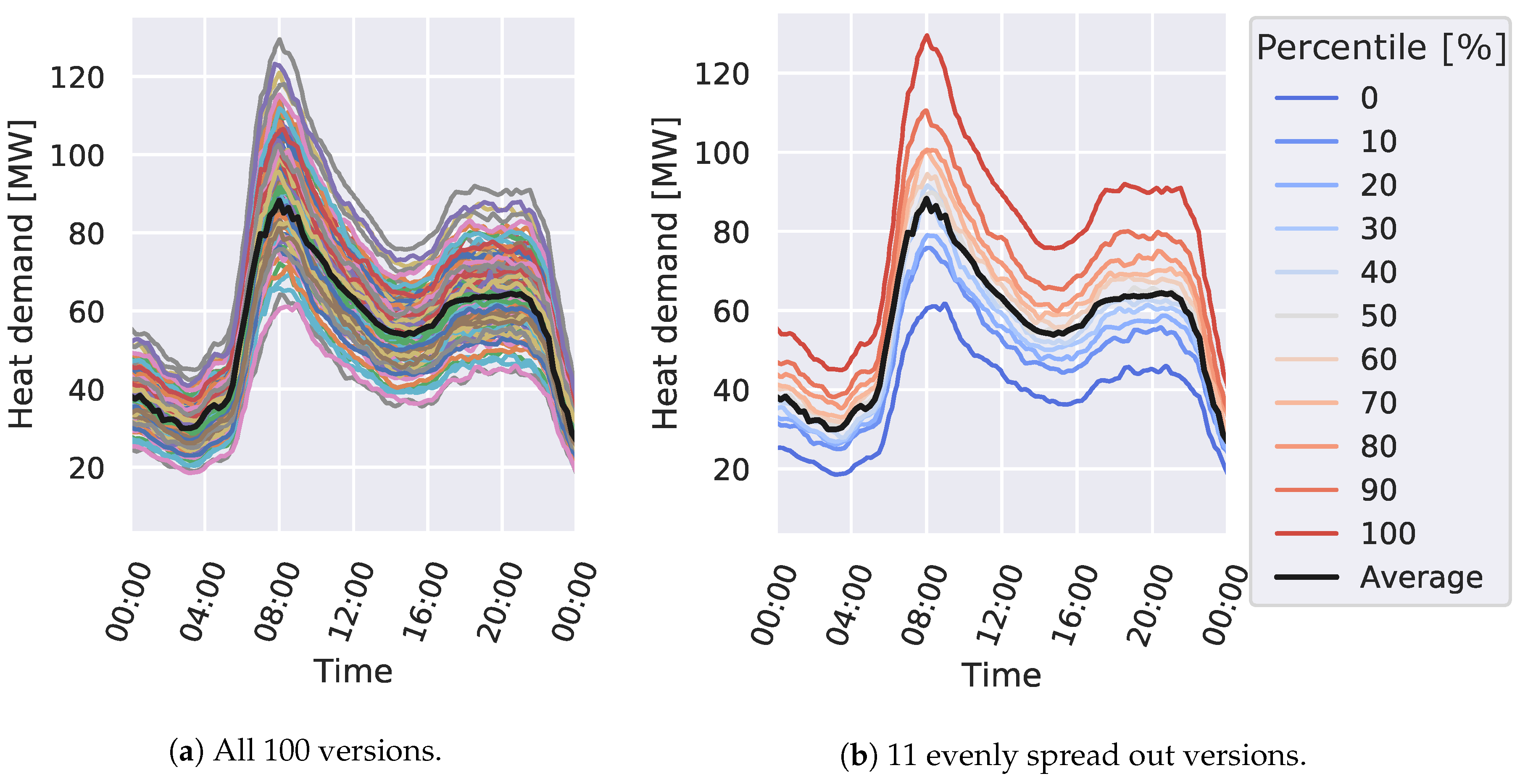
3.3. Uncertainty Analysis

Three steps are taken in order to analyse the influence of heat demand magnitude uncertainty on network flexibility activations, which are described below.

3.3.1. Step 1: Optimal Control of Each GenkNET  Version

With 100 possible versions of GenkNET created, the optimal control strategy of every version can be calculated. By solving the OCP twice, once with and once without network flexibility, referred to as the Flexibility and Reference cases, the optimal network flexibility activation can be isolated. Six days (see Table 1) will be analysed with respect to operational heat pump optimisation, and peak shaving for different base load ratios (60%, 80%, and 95%).

This leads to 100 optimal network flexibility activations for GenkNET, based on heat demand profiles that differ mostly in amplitude. This step will show how the optimal control changes as the heat demand magnitude changes. The nominal case mostly resembles version 50, which can be observed in several Figures. For an elaborate explanation on the nominal cases, the reader is referred to [50].

3.3.2. Step 2: Selection of 11 Control Strategies

All of the GenkNET versions are ordered from low to high annual heat demand. Using this ordering, every tenth profile is selected, corresponding to the selection in Figure 5b. Hence, when ordered according to the annual heat demand, versions 0, 10, 20, 30, 40, 50, 60, 70, 80, 90, and 100 are chosen. These versions will be named by these numbers in the remainder of this study, with 0 corresponding to the GenkNET version with the lowest annual heat demand and 100 to the one with the highest annual heat demand. Note that the ordering of the profiles is the same for each of the six days and any other variation that is analysed in this study.

3.3.3. Step 3: Applying the 11 Control Strategies to All 100 GenkNET  Versions

Finally, the optimal control strategies of the 11 versions that were selected in the previous step are applied to all 100 GenkNET versions. This leads to 1100 evaluations of GenkNET for one day and one optimisation case. This step shows how the optimal control performance changes when the ‘predicted’ and ‘actual’ heat demand differ from each other.

4. Results

The results are split up into a discussion of the optimisation of heat pump operation and peak shaving optimisation and they are presented below.

4.1. Operational Heat Pump Optimisation

The operation of the heat pump is optimised to achieve the lowest possible electricity costs to drive the heat pump while delivering the heat demand to the customers. The electricity prices are based on the 2014 BELPEX day-ahead electricity market.

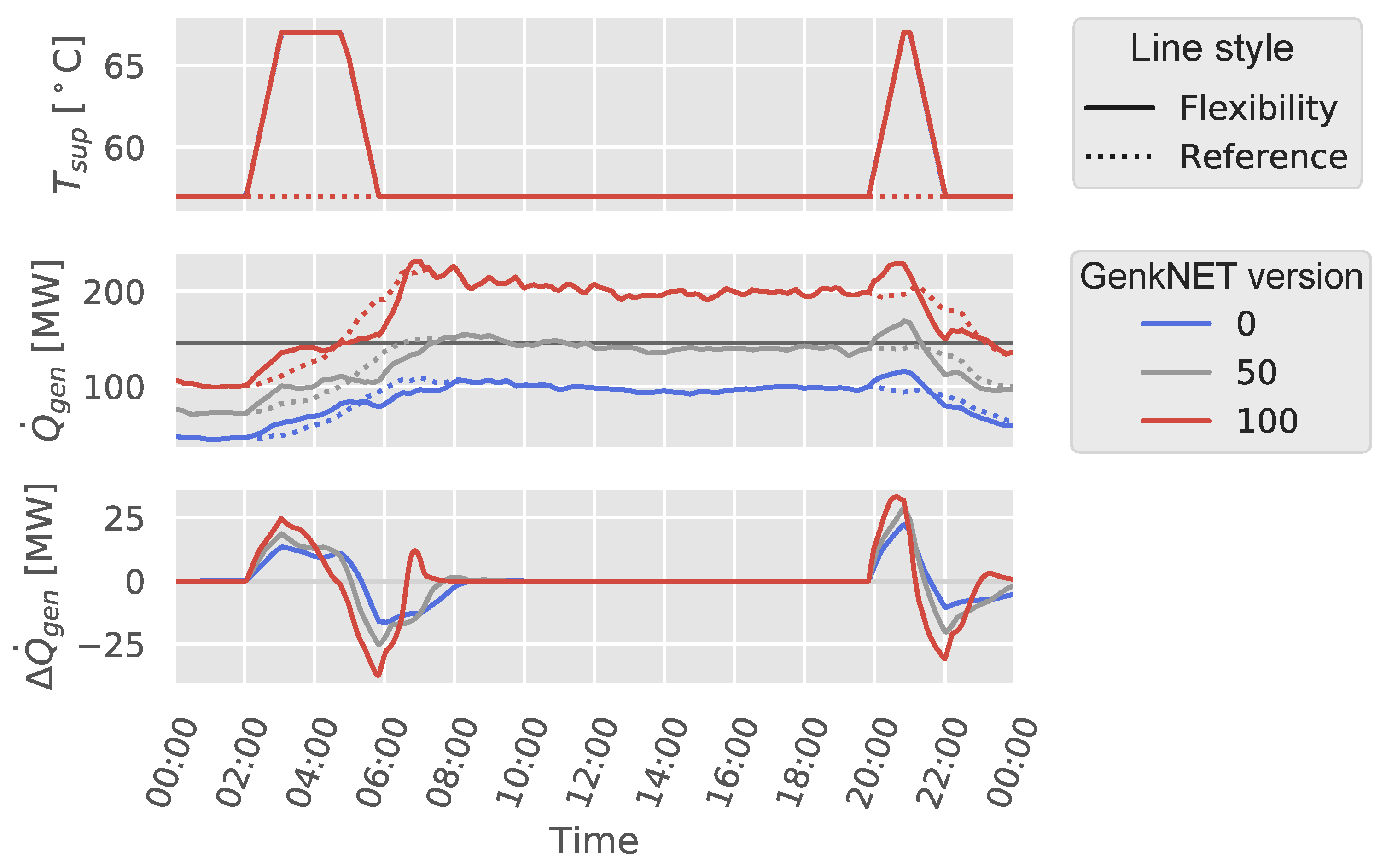
4.1.1. Optimal Control of the 11 Selected Versions

In Step 1 of the uncertainty analysis, the optimal control strategies of all 100 versions of GenkNET were calculated. Figure 6 shows the optimal control of the 11 selected versions on the Winter_Neg$p_e$ day (a winter day with an electricity price that becomes negative). These 11 versions are spread out over the entire range of heat demand magnitudes and they give a good overview of the optimal control of all versions. Figure 6 shows that the network is charged three times: during the two negative price periods and before a large change in electricity price. With the coefficient of performance (COP) reducing when the supply temperature is increased, which is inevitable when activating network flexibility, these are the only moments when network flexibility is profitable. In Figure 6, the Flexibility and Reference case refer to the cases in which network flexibility is available and in which it is unavailable, respectively.

During the first negative price period, there is a substantial difference between the supply temperature pulses of the different GenkNET versions, whereas the pulses are nearly identical in the second negative price period. The differences in the first period are likely caused by the second period that follows shortly after. In the low heat demand versions, the water travels so slowly that charging the network during the first negative period causes the network to discharge during the second, more interesting, negative period, which causes a loss in profits. In the high heat demand versions, the water travels faster and the discharge has ended by the time the second negative period starts.

When there is a large price difference, the supply temperature pulse remains similar in all cases but starts earlier as the heat demand reduces, again a consequence of the lower water speeds in the network. Hence, the general actions are largely based on the electricity price profile and remain similar throughout all versions. However, the exact timing can change considerably, with the pulse lengths doubling as the heat demand becomes lower. Note that the third pulse always ends at the same point in time, namely when the price increase is taking place.

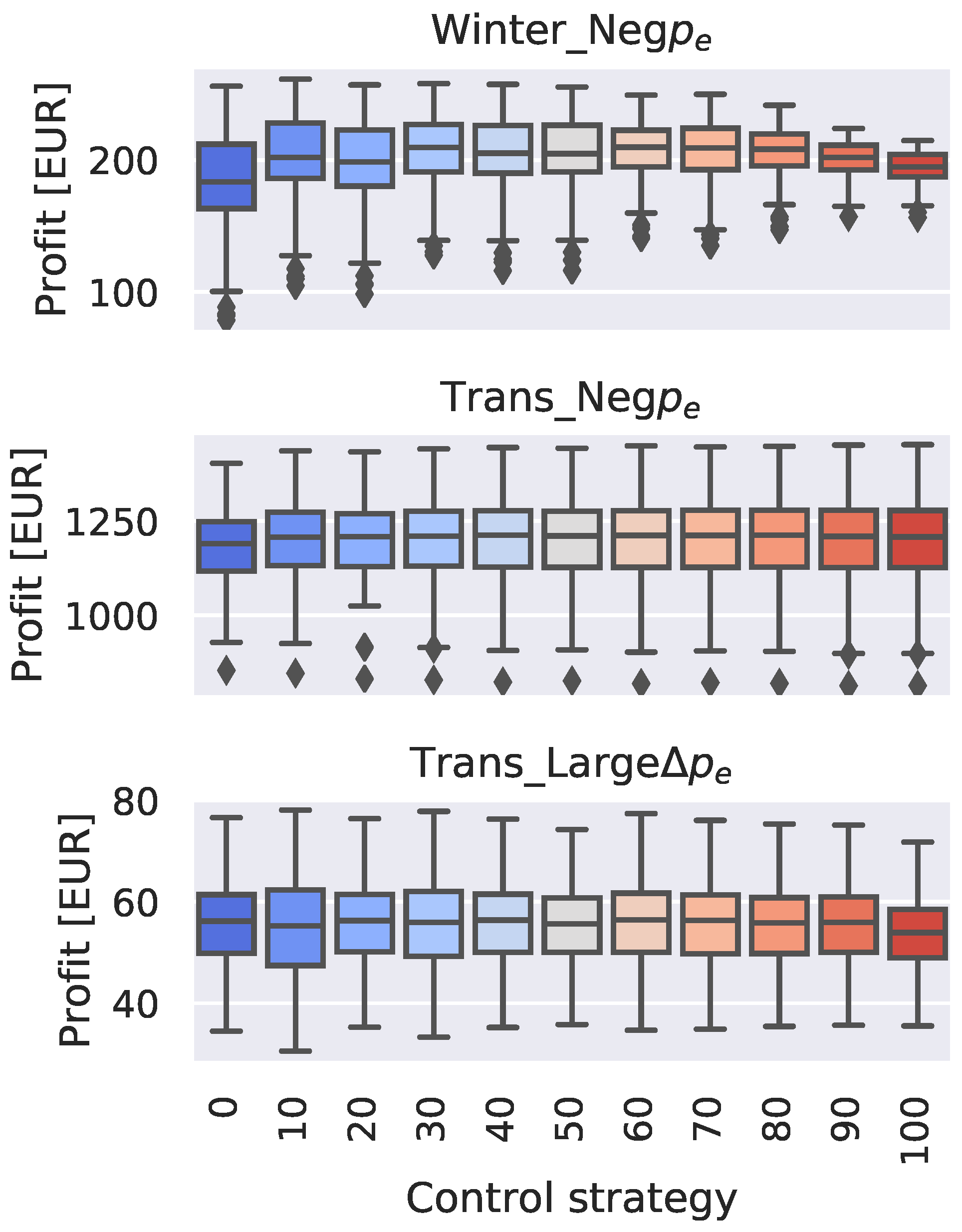
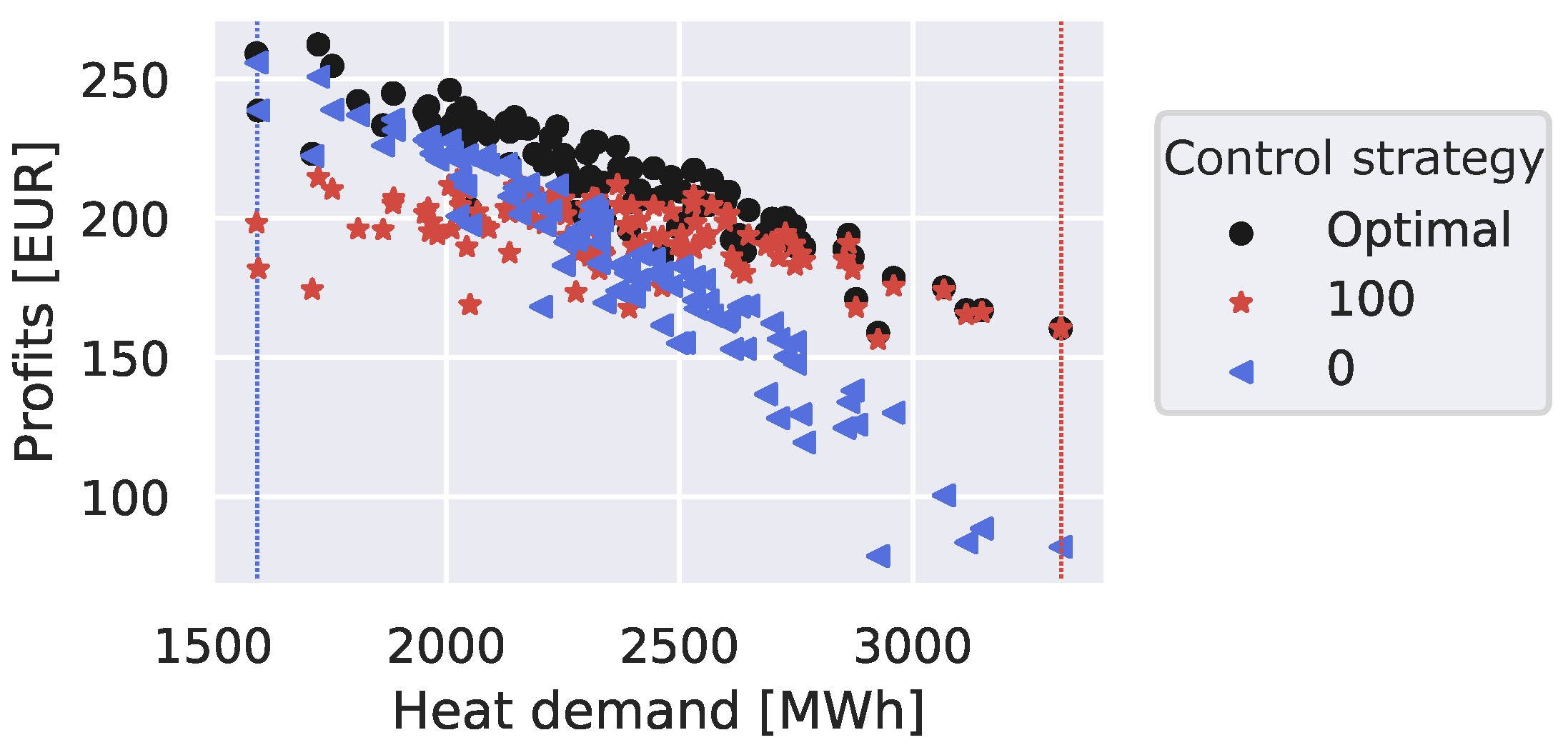
4.1.2. Applying 11 Different Control Strategies to All 100 GenkNET  Versions

In Step 3, the optimal supply temperature profiles in Figure 6 are applied to all 100 versions. This leads to 1100 evaluations for each day, which are presented in Figure 7. Only the three days during which there is a significant network flexibility activation are shown: Winter_Neg$p_e$, Trans_Neg$p_e$ and Trans_Large$\Delta p_e$. For each of the 11 selected control strategies, a box plot is set up. The box plot presents the profit of applying the selected control strategy to all GenkNET versions. Studying the median value, it seems that every optimal control strategy achieves a similar profit on average. On the Trans_Neg$p_e$ and Trans_Large$\Delta p_e$ days, the spread on the profits also remains similar, regardless of the control strategy. The profits are symmetrically spread around the median and show a possible deviation from the median profit of about 20% and 33% on Trans_Neg$p_e$ and Trans_Large$\Delta p_e$, respectively.

On the Winter_Neg$p_e$ day, the profit variation decreases as higher optimal control strategies are applied. Looking back at Figure 6, this is likely caused by the quick succession of two negative price periods. When a higher heat demand is predicted, a large supply temperature pulse is applied during the first negative period. If the actual heat demand is lower, the discharge phase is taking place during the more interesting second negative price period, thus limiting the profits. Vice versa, if a low heat demand is predicted, but it turns out to be high, the first negative price period was only covered by a small temperature pulse. The spread in profits for control strategies 0 and 100 can be seen in Figure 8, which also shows the difference with the actual optimal solution. It seems that an optimal control strategy that is based on a different heat demand prediction can lead to a profit reduction by up to a factor 2.

From the cases that are studied here, it seems that the risk related to heat demand magnitude uncertainty can cause a reduction in profits, yet there was no risk of losing money (negative profits). In general, the control strategy remained similar in all cases, as the control strategy mostly aims for moments with a negative price or with large price changes. The heat demand at those times seems less important.

4.2. Peak Shaving Optimisation

In the peak shaving optimisation, two plants are available to generate the heat. The base unit can generate heat cheaply, but it does not have a heat output that is sufficiently large to deliver the heat demand peaks. The peak unit can cover the peak but at a higher cost. To minimise the cost of heat generation, peak shaving is hence applied by activating network flexibility.

4.2.1. Optimal Control of the 11 Selected Versions

Figure 9 shows the optimal control results of the 11 selected profiles when the base unit can deliver 95% of the expected peak heat demand, with a peak-base price ratio of 2 on the Winter_Large$\Delta p_e$ day. It shows that the versions with a lower heat demand do not require any network flexibility, while those with a higher heat demand do not succeed in shaving the entire peak. For the versions with the highest heat demand, an additional large supply temperature pulse appears at the end of the peak period. As explained in [6], a flexibility activation takes place in several phases. First, the network is charged, then it is discharged and at the end a rebound takes place. The rebound compensates the part of the discharge that was not covered by the initial charge. In the last network flexibility activation at the end of the peak period in Figure 9, the initial charge and discharge are both covered by the peak unit, but the rebound is covered by the base unit, effectively moving a small amount of energy from the peak unit to the base unit.

The differences between the different control strategies are clearly larger than for the operational heat pump optimisation. Hence, it is expected that larger ranges of profits (and losses) will appear when applying these strategies to all 100 versions.

4.2.2. Applying 11 Different Control Strategies to All 100 GenkNET  Versions

Figure 10 shows the peak energy that could be avoided in all 100 versions with 11 different control strategies. This is done for the Winter_Large$\Delta p_e$ and Trans_Small$\Delta p_e$ days for base load ratios of 60%, 80%, and 95%. The variation in avoided peak energy has a much larger range than the profit range found for the operational heat pump optimisation. When comparing base load ratios, different trends can be observed.

Starting on the right of Figure 10 with a base load ratio of 95%, the lower control strategies cannot accomplish anything at all. Looking back at Figure 9, no network flexibility is required when the heat demand is low; hence, there is no network flexibility activation. Going to the higher control strategies, the average peak energy that can be avoided increases as does the possible range, although it always remains mostly positive, i.e., very little to no extra peak energy had to be generated even in the worst case for Trans_Small$\Delta p_e$.

However, the highest control strategies on Winter_Large$\Delta p_e$ cause extra amounts of peak energy to be generated in many cases. Here, a second large temperature pulse at the end of the peak period has appeared (see Figure 9). This type of network flexibility appears to entail a large risk, as illustrated in Figure 11. If this second pulse is applied to a case with a lower heat demand in which the peak unit is not active at that time, then the peak unit might have to be (re)activated in order to deliver this pulse while the base load is later on reduced, e.g., in version 50. This substantially increases the delivered peak energy. It seems that, in the case of a large base unit and heat demand magnitude uncertainties, it is better to overestimate than underestimate the heat demand, but to avoid a network flexibility activation at the end of a peak period.

Going to a base load ratio of 80%, a similar pattern appears, yet everything has shifted to the left; the base unit must now be activated more quickly. The Winter_Large$\Delta p_e$ day again shows a risk for generating more peak energy when going to higher control strategies. Again, this is caused by a network flexibility activation at the end of a peak period. This extra pulse has disappeared again at the highest control strategy, which shows no risk to increase the peak energy. The 80% case shows a clear best result in the intermediate control strategies. For these strategies, the heat demand was high enough that peak shaving is required, but not that high that the peak unit must be active (nearly) all the time, limiting chances for network flexibility.

In the case of 60%, another shift to the left has occurred, the peak unit is now activated even in case of the smallest heat demand. The average avoided peak energy now remains very constant up to the highest control strategies. Here, it decreases again, as hardly any network flexibility is activated any more. The heat demand has now become so high that the base unit must be active (nearly) all the time. Although the range of possible peak energy avoided can be large, there is little risk, i.e., the delivered peak energy will not increase. It seems that in case of a smaller base unit, it would be safe to underestimate the heat demand when deciding a control strategy.

In order to better understand what occurs when the heat demand changes and what influence the different control strategies have, Figure 12 shows the peak energy that could be avoided for all GenkNET cases in six days for a base load ratio of 95%. For each GenkNET version, the result of four different control strategies is shown: the optimal control strategy of that version, the result when the lowest and highest heat demand are ‘predicted’ and lastly a control strategy that follows the recommendations from before. For a base load ratio of 95%, it seemed to be advisable to select a control strategy that corresponds to a higher heat demand, without going too high. Hence, control strategy 70 is selected.

The optimal control solutions (black dots) presented in Figure 12 show some interesting results. With low heat demands, there is no need for peak shaving and, hence, no peak energy can be avoided either. After a while, the avoided peak starts increasing, until on most days a maximum is reached. This maximum corresponds to the maximum energy storage capacity of the GenkNET network. The maximum energy storage capacity is estimated to be $36.8$ $\mathrm{M}$$\mathrm{Wh}$, based on calculating the total water mass in the GenkNET network, see Figure 2, and multiplying this mass with the specific heat capacity of water and the allowed temperature increase of 10 ${}^{\circ }\mathrm{C}$. When this maximum energy storage capacity is exceeded, there are multiple peaks and network flexibility activations during one day, e.g., a morning and evening peak. These extra peaks appear and disappear as the heat demand magnitude changes.

Of all the control strategies, the optimal control strategy (black dots) reaches the best result in all cases, as is expected. Control strategy 0 cannot avoid any peak energy, as it does not activate network flexibility. Control strategy 100 can accomplish a reasonable result on the transitional days, noticing the afternoon peak that occurs with the highest heat demands on Trans_Neg$p_e$. However, on the winter days, it attempts to activate network flexibility at the end of a peak unit activation, which is risky in case the heat demand turns out to be lower. Lastly, when control strategy 70 is applied, it can, in most cases, follow the optimal strategy very well. It only misses the afternoon peak of Trans_Small$\Delta p_e$ and Trans_Neg$p_e$. On Winter_Small$\Delta p_e$, its performance decreases with increasing heat demand. Here, the peak period moves significantly through time as the heat demand changes. In the case of the highest heat demands, the peak has already started by the time case 70 starts charging the network. This implies that the changes in peak timing will complicate the selection of a robust control strategy even further.

Remember that each GenkNET version is composed of nine neighbourhoods, of which the heat demand variation was chosen at random and independently of the other neighbourhoods. This means that two GenkNET versions with equal total daily heat demand, could have a different distribution of heat demand throughout the nine neighbourhoods and a different reaction to the same supply temperature pulse. Yet, in Figure 12, all of the points show clear trends. It seems that a different heat demand distribution amongst the GenkNET neighbourhoods does not influence the network flexibility activation that much with the currently imposed building parameter distributions.

5. Discussion

This study investigates how optimal control changes when the building parameters and, hence, the heat demand magnitude changes and how the control performance changes when a control strategy that is based on a different ’predicted’ heat demand is applied. The results presented in this work are based on a tree-shaped network topology. Although there is no indication that the results do not apply to other networks, further research is highly recommended for meshed networks, distributed generation, etc.

5.1. How Does the Optimal Network Flexibility Activation Change When the Building Parameters/Heat Demand Magnitude Changes?

When the heat demand changes so do the mass flow rates and the network flexibility timing. This is an effect that is visible in the operational heat pump optimisations, although its influence is limited when electricity prices become negative. Only in certain circumstances when multiple negative price periods follow each other shortly, the heat demand magnitude may influence the network flexibility activation to a larger extent.

In the case of peak shaving, not only the mass flow rates in the system are important, so is the magnitude of the heat demand with respect to the maximum heat output of the base unit. This can largely influence the network flexibility activation. With a low heat demand, it may be that there is no need for peak shaving, while, with a high heat demand network, flexibility is not sufficient for shaving the entire peak.

5.2. How Does the Network Flexibility Performance Change When the Control Strategy Changes?

There was relatively little difference in the performance of different control strategies for operational heat pump optimisation.The resulting (average) profits were rather independent of the applied control strategy. Again, in the considered cases, it seems that the electricity price timing is at least as important as the heat demand magnitude. Only in special cases (with multiple negative price periods), a significant difference in control strategy performance could be noticed. Hence, for the case of GenkNET with variations on building parameters, operational heat pump optimisation does not present much risk. A minimum profit could be guaranteed in all cases.

For peak shaving, another observation can be made. The control strategies were highly dependent on the heat demand magnitude. Yet, an analysis of their performance (i.e., the peak energy that could be shaved) showed that the studied heat demand uncertainty does not introduce much risk. With most control strategies, the generated peak energy remained the same or decreased. In the few cases where network flexibility accomplished a result worse than the Reference case, this was caused by a network flexibility activation at the end of a peak period, or by a large change in the start time of a peak period. This does suggest that uncertainties in timing (related to user behaviour and weather), may induce larger risks.

5.3. Does This Preliminary Study Lead to Insights for a More Robust Activation of Network Flexibility?

For operational heat pump optimisation, it seems electricity price related uncertainties may be more relevant. Future research should look into this type of uncertainty in more detail in order to conclude what measures are required to achieve a more robust network flexibility activation. For now, considering only building parameter uncertainties, there seems to be little risk in selecting a control strategy.

For peak shaving, if only heat demand magnitude uncertainties are expected, then a recommendation for peak shaving can be made based on the results gathered in this paper. The losses associated with activating network flexibility needlessly are limited, while the possible gains are substantial. Hence, it seems better to activate too much flexibility, instead of too little. Only the activation at the end of a peak period should be avoided as it introduces a risk of generating more peak energy.

5.4. Remarks

This study only considers uncertainties on building parameters. Yet, in reality, these uncertainties may be the least problematic with respect to control. As building parameters do not change, the errors in heat demand predictions that are caused by them can be corrected over time. By contrast, the user behaviour and weather do change over time and may be much harder to deal with. However, for building parameter data, realistic data distributions could be set up and analysed.

The plant models are simple and do not contain all relevant aspects. For example, the peak unit may require start-up and shut-down costs. These costs increase the risk that is associated with heat demand uncertainties, as a small peak unit activation may cost much more than was assumed now. Additionally, it was assumed that the base unit can increase the network supply temperature without a reduced efficiency. If the efficiency depends on the supply temperature, this may alter the conclusions made before. Similar things can be said for the heat pump, for ramping limits and costs, etc. A future study should look into these aspects.

The building heat demand profiles were built with small random variations, along with uncorrelated building parameter uncertainties between the neighbourhoods. The results suggest that these aspects have little influence, as the scatter plots of Figure 8 and Figure 12 showed clear trends when ordering the different versions according to the total heat demand during the day. This would indicate that (1) small (random) heat demand variations may not be that important. Hence, predictions may not need to go in great detail, although the extent of this should be investigated. (2) The distribution of the heat demand among the neighbourhoods may not have such a large influence either, although the different neighbourhood locations in the network do influence the network flexibility activation timing. Again, this is another aspect that merits further study.

6. Conclusions

This study evaluates the influence of building parameter uncertainties on network flexibility performance. This is done by determining and analysing the distributions for building parameters in the city of Genk, Belgium. This led to 100 different profiles describing the heat demand in a fictive DH system in Genk. These heat demand profiles mostly differ in magnitude, not in timing. The optimal control strategy applying network flexibility for these different heat demand profiles was calculated for operational heat pump optimisation and peak shaving. Additionally, control strategies that are optimal for one heat demand profile were applied to all others, in order to study the influence of an incorrect heat demand prediction.

The analysis of these results shows that building parameter uncertainties do not influence operational heat pump optimisation much, and could reach an average profit that is similar regardless of the applied control strategy. For peak shaving, the heat demand magnitude matters much more, as it is the main factor that determines a peak unit activation. Yet, here, the risk remains limited; hence, a large network flexibility activation to prevent a possible peak period seems advisable.

References

1. European Commission. Statistical office of the European Union; European Commission: Brussels, Belgium, 2019. [Google Scholar]
2. Fleiter, T.; Steinbach, J.; Ragwitz, M. Mapping and Analyses of the Current and Future (2020–2030) Heating/Cooling Fuel Deployment. Available online: https://ec.europa.eu/energy/studies/mapping-and-analyses-current-and-future-2020-2030-heatingcooling-fuel-deployment_en (accessed on 25 November 2020).
3. European Commission. An EU Strategy on Heating and Cooling; European Commission: Brussels, Belgium, 2016. [Google Scholar]
4. Frederiksen, S.; Werner, S. District Heating and Cooling; Studentlitteratur: Lund, Sweden, 2014. [Google Scholar]
5. Connolly, D.; Lund, H.; Mathiesen, B.V.; Werner, S.; Möller, B.; Persson, U.; Boermans, T.; Trier, D.; Østergaard, P.A.; Nielsen, S. Heat Roadmap Europe: Combining district heating with heat savings to decarbonise the EU energy system. Energy Policy 2014, 65, 475–489. [Google Scholar] [CrossRef]
6. Vandermeulen, A.; Van Oevelen, T.; van der Heijde, B.; Helsen, L. A simulation-based evaluation of substation models for network flexibility characterisation in district heating networks. Energy 2020, 117650. [Google Scholar] [CrossRef]
7. Vandermeulen, A.; van der Heijde, B.; Helsen, L. Controlling district heating and cooling networks to unlock flexibility: A review. Energy 2018, 151, 103–115. [Google Scholar] [CrossRef]
8. Giraud, L.; Merabet, M.; Baviere, R.; Vallée, M. Optimal Control of District Heating Systems using Dynamic Simulation and Mixed Integer Linear Programming. In Proceedings of the 12th International Modelica Conference, Prague, Czech Republic, 15–17 May 2017; pp. 141–150. [Google Scholar] [CrossRef] [Green Version]
9. Bavière, R.; Vallée, M. Optimal Temperature Control of Large Scale District Heating Networks. Energy Procedia 2018, 149, 69–78. [Google Scholar] [CrossRef]
10. Ikonen, E.; Selek, I.; Kovacs, J.; Neuvonen, M.; Szabo, Z.; Bene, J.; Peurasaari, J. Short term optimization of district heating network supply temperatures. In Proceedings of the ENERGYCON 2014—IEEE International Energy Conference, Dubrovnik, Croatia, 13–16 May 2014; pp. 996–1003. [Google Scholar] [CrossRef]
11. Benonysson, A.; Bøhm, B.; Ravn, H.F. Operational optimization in a district heating system. Energy Convers. Manag. 1995, 36, 297–314. [Google Scholar] [CrossRef]
12. Laakkonen, L.; Korpela, T.; Kaivosoja, J.; Vilkko, M.; Majanne, Y.; Nurmoranta, M. Predictive Supply Temperature Optimization of District Heating Networks Using Delay Distributions. Energy Procedia 2017, 116, 297–309. [Google Scholar] [CrossRef]
13. Leśko, M.; Bujalski, W.; Futyma, K. Operational optimization in district heating systems with the use of thermal energy storage. Energy 2018, 165, 902–915. [Google Scholar] [CrossRef]
14. Dominković, D.F.; Junker, R.G.; Lindberg, K.B.; Madsen, H. Implementing flexibility into energy planning models: Soft-linking of a high-level energy planning model and a short-term operational model. Appl. Energy 2020, 260, 114292. [Google Scholar] [CrossRef]
15. Gu, W.; Wang, J.; Lu, S.; Luo, Z.; Wu, C. Optimal operation for integrated energy system considering thermal inertia of district heating network and buildings. Appl. Energy 2017, 199, 234–246. [Google Scholar] [CrossRef]
16. Li, Z.; Wu, W.; Shahidehpour, M. Combined Heat and Power Dispatch Considering Pipeline Energy Storage of District Heating Network. IEEE Trans. Sustain. Energy 2016, 7, 12–22. [Google Scholar] [CrossRef]
17. Tian, L.; Xie, Y.; Hu, B.; Liu, X.; Deng, T.; Luo, H.; Li, F. A Deep Peak Regulation Auxiliary Service Bidding Strategy for CHP Units Based on a Risk-Averse Model and District Heating Network Energy Storage. Energies 2019, 12, 3314. [Google Scholar] [CrossRef] [Green Version]
18. Kim, S.H. An evaluation of robust controls for passive building thermal mass and mechanical thermal energy storage under uncertainty. Appl. Energy 2013, 111, 602–623. [Google Scholar] [CrossRef]
19. Baetens, R.; Saelens, D. Modelling uncertainty in district energy simulations by stochastic residential occupant behaviour. J. Build. Perform. Simul. 2015, 1493, 1–17. [Google Scholar] [CrossRef]
20. Strathclyde University. Demand Profile Generator. Available online: http://www.esru.strath.ac.uk/EandE/Web_sites/06-07/Carbon_neutral/tools%20folder/introduction.htm (accessed on 25 November 2020).
21. Rysanek, A.M.; Choudhary, R. DELORES—An open-source tool for stochastic prediction of occupant services demand. J. Build. Perform. Simul. 2015, 8, 97–118. [Google Scholar] [CrossRef]
22. Yamaguchi, Y.; Kambayashi, Y.; Okada, T.; Shoda, Y.; Shimoda, Y. Community-Scale Household Activity Modelling Considering Household Heterogeneity Using Japanese Time Use Data. In Proceedings of the Urban Energy Simulation Conference, San Francisco, CA, USA, 6–8 September 2017; pp. 1–6. [Google Scholar]
23. Oldewurtel, F. Stochastic Model Predictive Control for Energy Efficient Building Climate Control. Ph.D. Thesis, ETH Zurich, Zurich, Switzerland, 2011. [Google Scholar]
24. Reinhart, C.F.; Cerezo Davila, C. Urban building energy modeling—A review of a nascent field. Build. Environ. 2016, 97, 196–202. [Google Scholar] [CrossRef] [Green Version]
25. Kavgic, M.; Mavrogianni, A.; Mumovic, D.; Summerfield, A.; Stevanovic, Z.; Djurovic-Petrovic, M. A review of bottom-up building stock models for energy consumption in the residential sector. Build. Environ. 2010, 45, 1683–1697. [Google Scholar] [CrossRef]
26. Cuypers, D.; Vandevelde, B.; Van Holm, M.; Verbeke, S. Belgische Woningtypologie: Nationale Brochure over de TABULA Woningtypologie; Technical Report. Mol, Belgium, 2014. Available online: http://episcope.eu/fileadmin/tabula/public/docs/brochure/BE_TABULA_TypologyBrochure_VITO.pdf (accessed on 31 July 2020).
27. De Jaeger, I.; Lago, J.; Saelens, D. A probabilistic building characterization method for district energy simulations. Energy Build. 2021, 230, 110566. [Google Scholar] [CrossRef]
28. De Coninck, R.; Helsen, L. Practical implementation and evaluation of model predictive control for an office building in Brussels. Energy Build. 2016, 111, 290–298. [Google Scholar] [CrossRef]
29. Arnold, M.; Andersson, G. Model Predictive Control of Energy Storage including Uncertain Forecasts. In Proceedings of the Power Systems Computation Conference (PSCC), Stockholm, Sweden, 22–26 August 2011; pp. 24–29. [Google Scholar]
30. Bruninx, K.; Patteeuw, D.; Delarue, E.; Helsen, L.; D’Haeseleer, W. Short-term demand response of flexible electric heating systems: The need for integrated simulations. In Proceedings of the IEEE International Conference on the European Energy Market (EEM), Stockholm, Sweden, 27–31 May 2013; pp. 28–30. [Google Scholar] [CrossRef]
31. Verrilli, F.; Parisio, A.; Glielmo, L. Stochastic Model Predictive Control for Optimal Energy Management of District Heating Power Plants. In Proceedings of the 2016 IEEE 55th Conference on Decision and Control, Las Vegas, NV, USA, 12–14 December 2016. [Google Scholar]
32. Wang, C.; Jiao, B.; Guo, L.; Tian, Z.; Niu, J.; Li, S. Robust scheduling of building energy system under uncertainty. Appl. Energy 2016, 167, 366–376. [Google Scholar] [CrossRef]
33. Gao, D.C.; Sun, Y.; Lu, Y. A robust demand response control of commercial buildings for smart grid under load prediction uncertainty. Energy 2015, 93, 275–283. [Google Scholar] [CrossRef]
34. Rosenblueth, E. Point estimates for probability moments. Proc. Natl. Acad. Sci. USA 1975, 72, 3812–3814. [Google Scholar] [CrossRef] [PubMed] [Green Version]
35. Massrur, H.R.; Niknam, T.; Fotuhi-Firuzabad, M. Investigation of Carrier Demand Response Uncertainty on Energy Flow of Renewable-Based Integrated Electricity-Gas-Heat Systems. IEEE Trans. Ind. Inform. 2018, 14, 5133–5142. [Google Scholar] [CrossRef]
36. Kitapbayev, Y.; Moriarty, J.; Mancarella, P. Stochastic control and real options valuation of thermal storage-enabled demand response from flexible district energy systems. Appl. Energy 2015, 137, 823–831. [Google Scholar] [CrossRef]
37. Diehl, M.; Gerhard, J.; Marquardt, W.; Mönnigmann, M. Numerical solution approaches for robust nonlinear optimal control problems. Comput. Chem. Eng. 2008, 32, 1279–1292. [Google Scholar] [CrossRef]
38. Lin, J.G.G. On min-norm and min-max methods of multi-objective optimization. Math. Program. 2005, 103, 1–33. [Google Scholar] [CrossRef]
39. Rantzer, J. Robust Production Planning for District Heating Networks. Master’s Thesis, Lund University, Lund, Sweden, 2015. [Google Scholar]
40. Vandermeulen, A.; van der Heijde, B.; Vanhoudt, D.; Salenbien, R.; Helsen, L. modesto—A Multi-Objective District Energy Systems Toolbox for Optimisation. In Proceedings of the Solar District Heating Conference, Graz, Austria, 11–12 April 2018. [Google Scholar]
41. Wang, H.; Lahdelma, R.; Wang, X.; Jiao, W.; Zhu, C.; Zou, P. Analysis of the location for peak heating in CHP based combined district heating systems. Appl. Therm. Eng. 2015, 87, 402–411. [Google Scholar] [CrossRef]
42. Basciotti, D.; Judex, F.; Pol, O.; Schmidt, R.R. Sensible heat storage in district heating networks: A novel control strategy using the network as storage. In Proceedings of the 6th International Renewable Energy Storage Conference IRES, Berlin, Germany, 28–30 November 2011. [Google Scholar]
43. Vandermeulen, A.; Reynders, G.; van der Heijde, B.; Vanhoudt, D.; Salenbien, R.; Saelens, D.; Helsen, L. Sources of energy flexibility in district heating networks: Building thermal inertia versus thermal energy storage in the network. In Proceedings of the Urban Energy Simulations Conference, Glasgow, UK, 30 November 2018. [Google Scholar]
44. Van der Heijde, B.; Vandermeulen, A.; Salenbien, R.; Helsen, L. Integrated Optimal Design and Control of Fourth Generation District Heating Networks with Thermal Energy Storage. Energies 2019, 12, 2766. [Google Scholar] [CrossRef] [Green Version]
45. Remmen, P.; Lauster, M.; Mans, M.; Fuchs, M.; Osterhage, T.; Müller, D. TEASER: An open tool for urban energy modelling of building stocks. J. Build. Perform. Simul. 2018, 11, 84–98. [Google Scholar] [CrossRef]
46. De Jaeger, I.; Reynders, G.; Ma, Y.; Saelens, D. Impact of building geometry description within district energy simulations. Energy 2018, 158, 1060–1069. [Google Scholar] [CrossRef]
47. Baetens, R.; De Coninck, R.; Jorissen, F.; Picard, D.; Helsen, L.; Saelens, D. OpenIDEAS—An Open Framework for Integrated District Energy Simulations. In Proceedings of the BS2015 14th Conference of International Building Performance Simulation Association, Hyderabad, India, 7–9 December 2015; pp. 347–354. [Google Scholar]
48. Serrano-Guerrero, X.; Escrivá-Escrivá, G.; Roldán-Blay, C. Statistical methodology to assess changes in the electrical consumption profile of buildings. Energy Build. 2018, 164, 99–108. [Google Scholar] [CrossRef]
49. Bünning, F.; Heer, P.; Smith, R.S.; Lygeros, J. Improved day ahead heating demand forecasting by online correction methods. Energy Build. 2020, 211. [Google Scholar] [CrossRef] [Green Version]
50. Vandermeulen, A. Quantification and Optimal Control of Network Flexibility in District Heating Systems. Ph.D. Thesis, KU Leuven, Leuven, Belgium, 2020. [Google Scholar]
51. Guelpa, E.; Sciacovelli, A.; Verda, V. Thermo-fluid dynamic model of large district heating networks for the analysis of primary energy savings. Energy 2019, 184, 34–44. [Google Scholar] [CrossRef] [Green Version]
52. Kudela, L.; Chylek, R.; Pospisil, J. Performant and simple numerical modeling of district heating pipes with heat accumulation. Energies 2019, 12, 633. [Google Scholar] [CrossRef] [Green Version]
53. Betancourt Schwarz, M.; Mabrouk, M.T.; Santo Silva, C.; Haurant, P.; Lacarrière, B. Modified finite volumes method for the simulation of dynamic district heating networks. Energy 2019, 182, 954–964. [Google Scholar] [CrossRef]
54. Borsche, R.; Eimer, M.; Siedow, N. A local time stepping method for thermal energy transport in district heating networks. Appl. Math. Comput. 2019, 353, 215–229. [Google Scholar] [CrossRef]
55. Rein, M.; Mohring, J.; Damm, T.; Klar, A. Optimal control of district heating networks using a reduced order model. arXiv 2019, arXiv:1907.05255. [Google Scholar] [CrossRef]
56. Sartor, K.; Thomas, D.; Dewallef, P. A comparative study for simulating heat transport in large district heating networks. Int. J. Heat Technol. 2018, 36, 301–308. [Google Scholar] [CrossRef]
57. Wang, Y.; You, S.; Zhang, H.; Zheng, X.; Zheng, W.; Miao, Q.; Lu, G. Thermal transient prediction of district heating pipeline: Optimal selection of the time and spatial steps for fast and accurate calculation. Appl. Energy 2017, 206, 900–910. [Google Scholar] [CrossRef]
58. Vivian, J.; Monsalvete Alvarez de Uribarri, P.; Eicker, U.; Zarrella, A. The effect of discretization on the accuracy of two district heating network models based on finite-difference methods. In Proceedings of the 16th International Symposium on District Heating an Cooling, Hamburg, Germany, 9–12 September 2018; pp. 1–10. [Google Scholar]
59. Bennonysson, A. Dynamic Modelling and Operation Optimization of District Heating Systems. Ph.D. Thesis, Technical University of Denmark, Lyngby, Denmark, 1991. [Google Scholar]
60. Van der Heijde, B.; Fuchs, M.; Ribas Tugores, C.; Schweiger, G.; Sartor, K.; Basciotti, D.; Müller, D.; Nytsch-geusen, C.; Wetter, M.; Helsen, L. Dynamic equation-based thermo-hydraulic pipe model for district heating and cooling systems. Energy Convers. Manag. 2017, 151, 158–169. [Google Scholar] [CrossRef] [Green Version]
61. European Standard. NBN EN 13941:2019 District Heating Pipes. Design and Installation of Thermal Insulated Bonded Single and Twin Pipe Systems for Directly Buried Hot Water Networks; NBN: Brussels, Belgium, 2019. [Google Scholar]
62. Wächter, A.; Biegler, L.T. On the implementation of an interior-point filter line-search algorithm for large-scale nonlinear programming. Math. Program. 2006, 106, 25–57. [Google Scholar] [CrossRef]
Figure 1. A flow chart describing the different steps taken to determine the GenkNET heat demand profiles including uncertainties (relevant to both Section 2 and Section 3).
Energies 13 06220 g001
Figure 2. The lay-out of the aggregated GenkNET, indicating the position of the nine neighbourhoods. There is a single heat generation site in the north-east of the network. The network pipes are indicated by the numbered lines.
Energies 13 06220 g002
Figure 3. Five histograms showing the building parameter distribution in the nine GenkNET neighbourhoods, according to the 9 × 500 variations.
Energies 13 06220 g003
Figure 4. A histogram showing the distribution of the annual GenkNET heat demand, according to the 500 variations.
Energies 13 06220 g004
Figure 5. The different heat demand profiles of GenkNET for the Trans_Neg p e day. The black line indicates the expected heat demand.
Energies 13 06220 g005
Figure 6. For the Winter_Neg p e day, the results of the operational heat pump optimisation for the 11 selected GenkNET versions are shown. From top to bottom, the electricity price, the supply temperature at the plant, the heat injection, and the heat injection response (the difference between the Flexibility and Reference case) are shown. The negative price periods are indicated by the dark grey zones.
Energies 13 06220 g006
Figure 7. Box plots of the profits obtained with the 11 selected control strategies on all GenkNET versions for three different days. The box plots shows the median, first and third quartile and the minimum and maximum (excluding outliers) of a data set. The outliers are represented by the diamond markers.
Energies 13 06220 g007
Figure 8. On the x-axis the heat demand during the Winter_Neg p e day is shown, on the y-axis the profit that was obtained. Every dot represents one version of GenkNET managed by one control strategy, the colour and marker shape indicate the applied control strategy. One version will always have the same heat demand, regardless of the applied control strategy. The vertical dotted lines show the heat demand that corresponds to the 0 and 100 control strategies.
Energies 13 06220 g008
Figure 9. For the Winter_Large Δ p e day, the results of the base-peak plant optimisation for the 11 selected GenkNET versions with a base load ratio of 95% are shown. From top to bottom, the supply temperature at the plant, the heat injection and the heat injection response are shown. In the middle graph, the maximum heat output of the base unit is indicated by the grey horizontal line.
Energies 13 06220 g009
Figure 10. Box plots of the avoided peak energy with the 11 selected control strategies on all 100 versions of GenkNET for Winter_Large Δ p e and Trans_Small Δ p e and for different base load ratios.
Energies 13 06220 g010
Figure 11. The application of control strategy 100 on a GenkNET version with low (0), medium (50) and high (100) heat demand on the Winter_Large Δ p e day with a base load ratio of 95%. The maximum base unit heat generation is indicated by the horizontal grey line.
Energies 13 06220 g011
Figure 12. On the x-axis the total heat demand during each day and each version is shown, on the y-axis the peak energy that was avoided with a control strategy. Every dot represents one version of GenkNET managed by a different control strategy. The vertical dotted lines show the heat demand that corresponds to the shown control strategies.
Energies 13 06220 g012