3.1. Classification of the Current–Voltage (I–V) Curves of the PV Panels
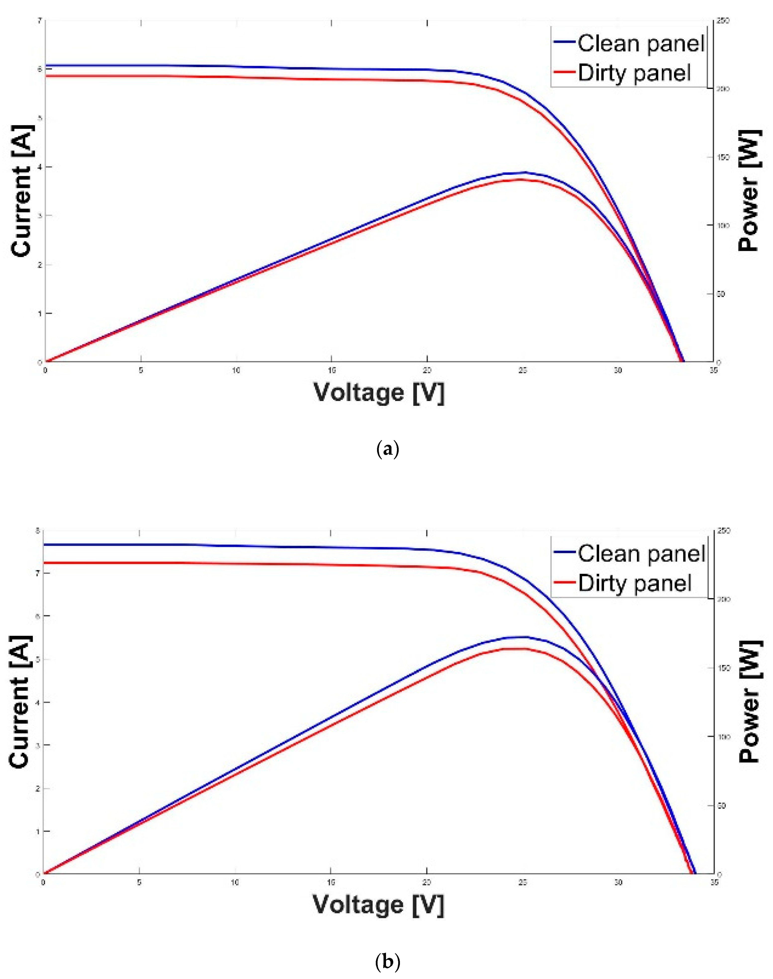
To begin with, a pair of curves taken from clear days in different months are presented to analyze the variation in the characteristic parameters throughout the acquisition campaign.
Figure 3 corresponds to the curves measured on 17 January and 14 March, where the
x-axis shows the voltage, the primary
y-axis the short circuit current and the
y-axis seconds the panel power.
Comparing the two images over time, one can see that the amount of dust deposition has increased, making the difference between the characteristic parameters for March greater than in January even though production was higher due to the higher incident radiation levels. These images also show how the short circuit current (a current equal to zero) is the parameter most affected by the dust deposition on the PV panels. In fact, this is the parameter used in several similar studies.
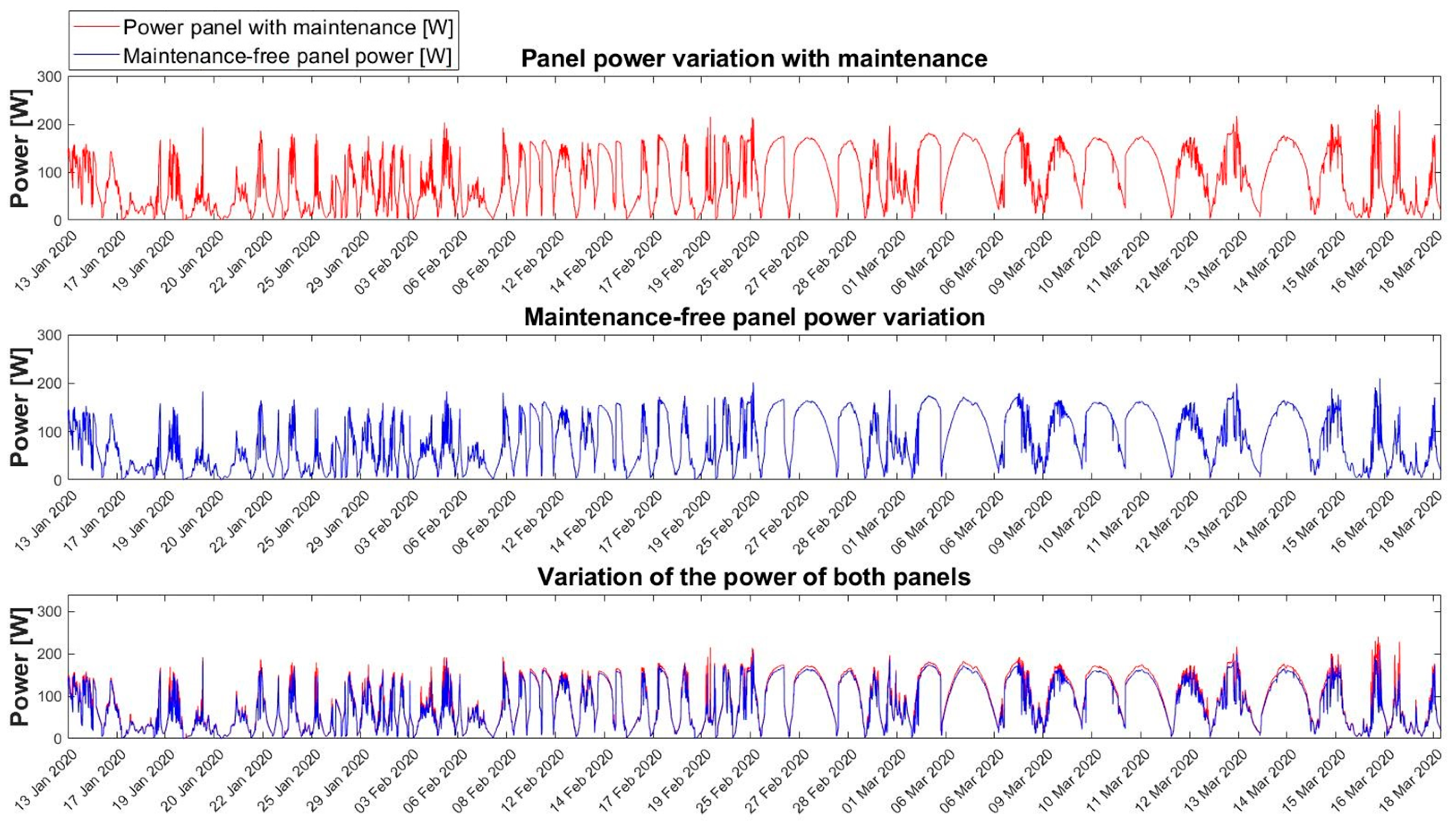
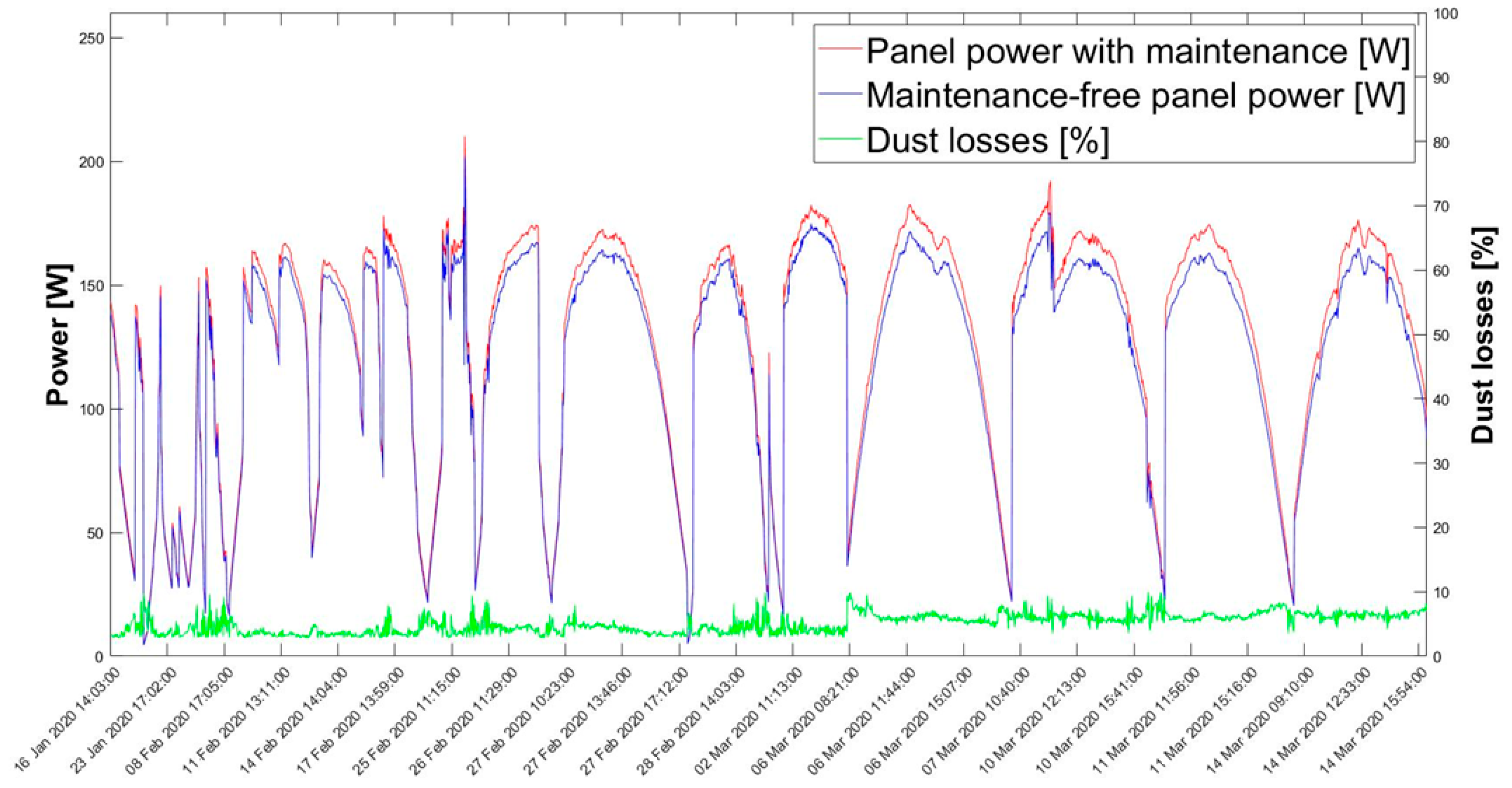
The graphs in
Figure 4 represent the maximum power of the PV panels (y-axel) studied at each moment (x-axel). The upper graph shows the variation in power of the panel with maintenance whereas the middle graph shows the variation in power of the panel without maintenance over the measurement campaign. In the lower graph, the two preceding graphs have been superimposed to show the difference in power existing between the two panels. At all times, the power of the panel with maintenance was higher than that for the panel without maintenance. It can also be seen how the power difference over time becomes greater as dirt accumulates; this is due to the lack of maintenance and heavy rainfall.
In this work, clear-day values were used since they are more suitable for calculating the variation in power loss; hence, there will be fewer errors in the final result.
3.2. Dust Losses
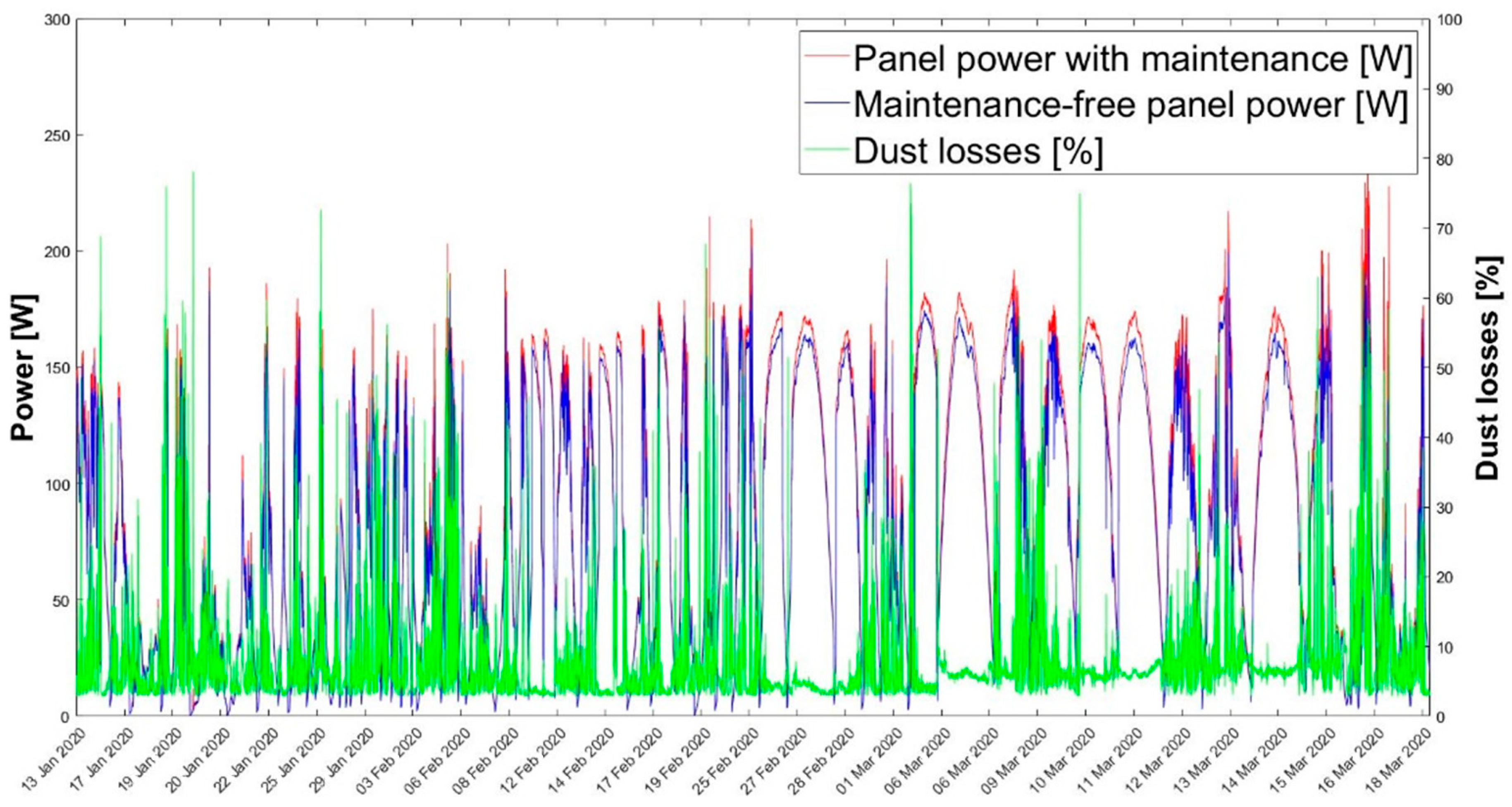
Once the power of each panel is known, the power loss can be determined according to Equation (1). As can be seen in
Figure 5, the variation in reduced power associated with dust pollution has noise in the sections where the incident radiation is low, where the
x-axis represents the measurement time, the primary
y-axis the power and the secondary
y-axis the dust losses.
This noise is due to integrating the error of the different signals required to calculate the power loss associated with dust deposition. As previously stated, these values correspond mainly to the times when the received radiation is low. At those moments, the determination of the different electrical parameters on which the power loss calculation is based, has been less precise. Consequently, we performed a filtering to eliminate the sections in which the variable contained noise.
Once the moments in the calculated production losses variable containing noise were discarded, the graph in
Figure 6 was obtained.
As can be observed, on most of the days in January and early February, there were cloud passages that made it difficult to determine the loss factor associated with dust contamination. However, on the remaining days, there are losses with lower peaks that make it possible to calculate a representative loss factor for the period under study.
The following average production soiling factors were obtained for each month, and for the entire study period: as shown in
Table 4, the factor increases with time, especially when there is no rainfall. The reduction factor for the month of March is the most precisely calculated since it is a month in which most of the days studied were clear, allowing it to be uniformly calculated. In addition, 11 June was one of the days when the sky was clear. After analyzing this day, it was observed that, due to the conditions in Almería, the panels were cleaned periodically due to rainfall, so the losses did not accumulate and, therefore, an annual adjustment cannot be made using the months analyzed.
Once the variation in the loss factor from dust was determined, the variation in the different recorded meteorological variables were represented, together with the power losses, to analyze the possible dependence between them.
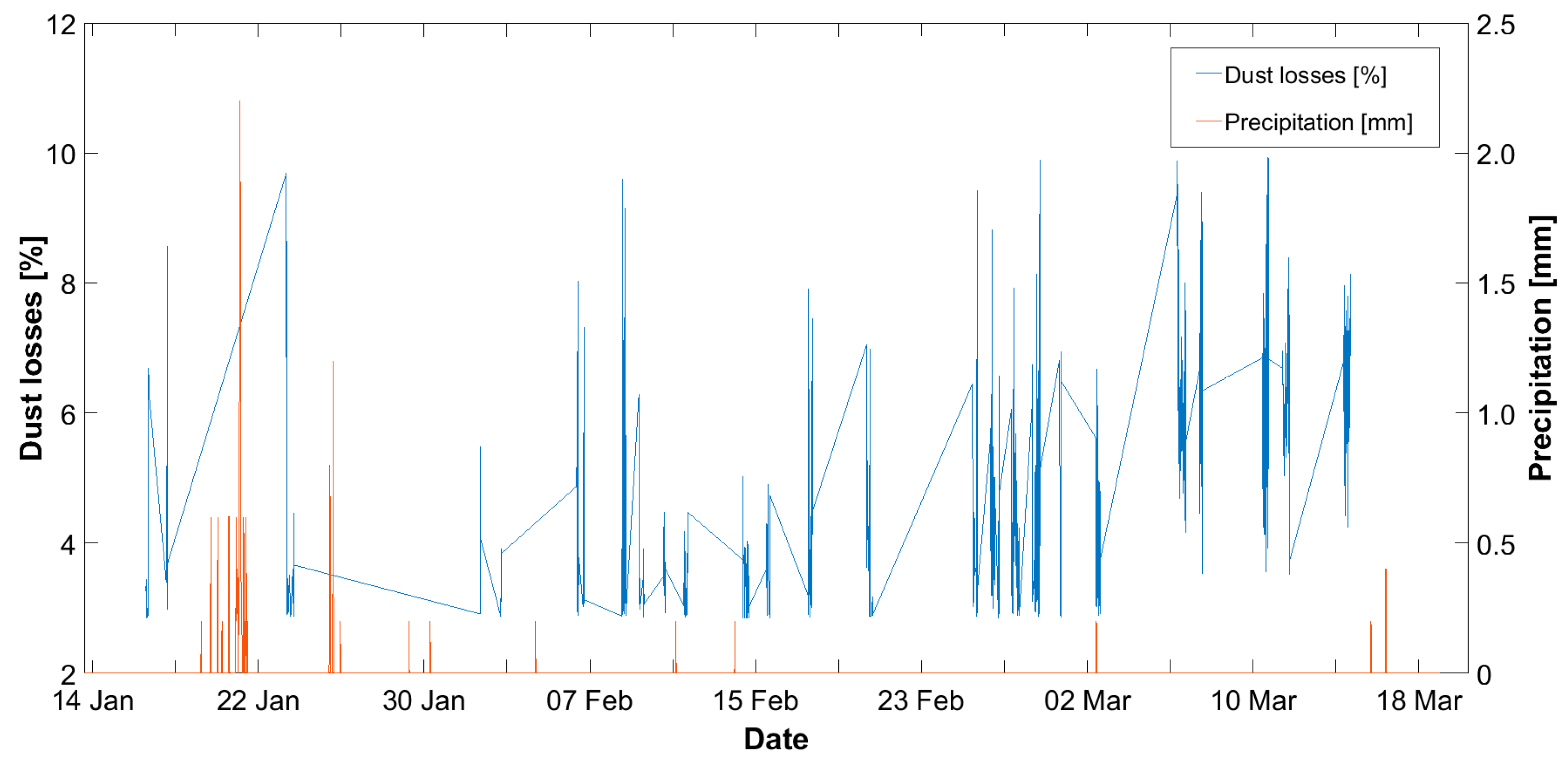
The rain episodes that occurred over the measurement campaign were represented in order to analyze their influence on the variation in the determined power losses (
Figure 7). In this graph, dust losses (primary
y-axis) and precipitation (secondary
y-axis) are represented against time (
x-axis).
The most important rains fell at the beginning of January, coinciding with the days when there was sky cover. At those moments, the signal noise is extremely high so most of the records for these days have been filtered out. Some rain episodes were also observed during the month of March although these were episodes in which little rain fell, having practically no repercussion on the variation in power loss.
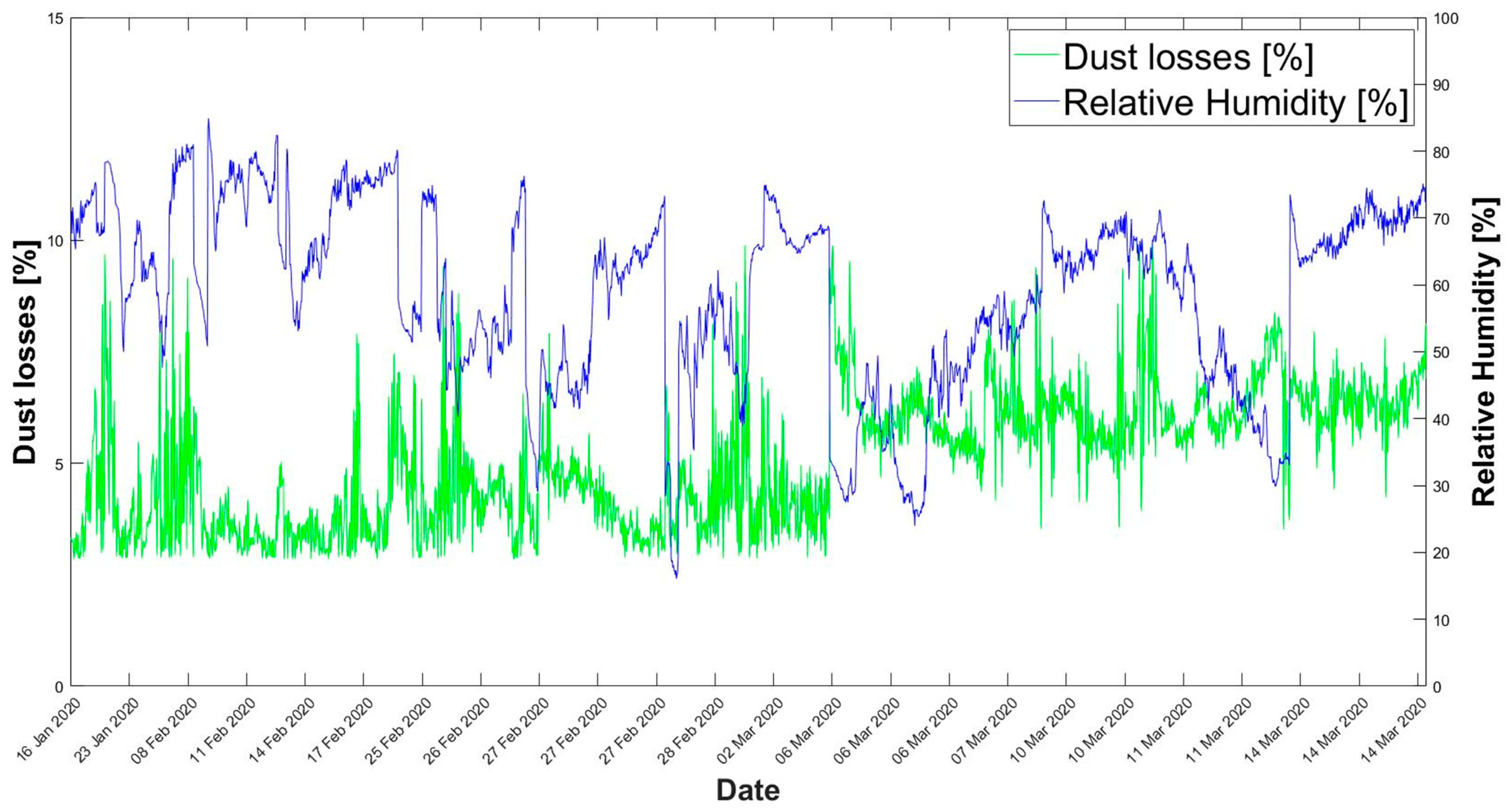
The dust losses (primary
y-axis) and relative humidity (secondary
y-axis) are shown against time (
x-axis) in
Figure 8.
A priori, no clear pattern can be observed between the two variables, although it can be stated that, at times when humidity is high due to rainfall (
Figure 7), dust losses are high; indeed, when there is rain, optimal conditions do not exist for determining the dust losses of the panels.
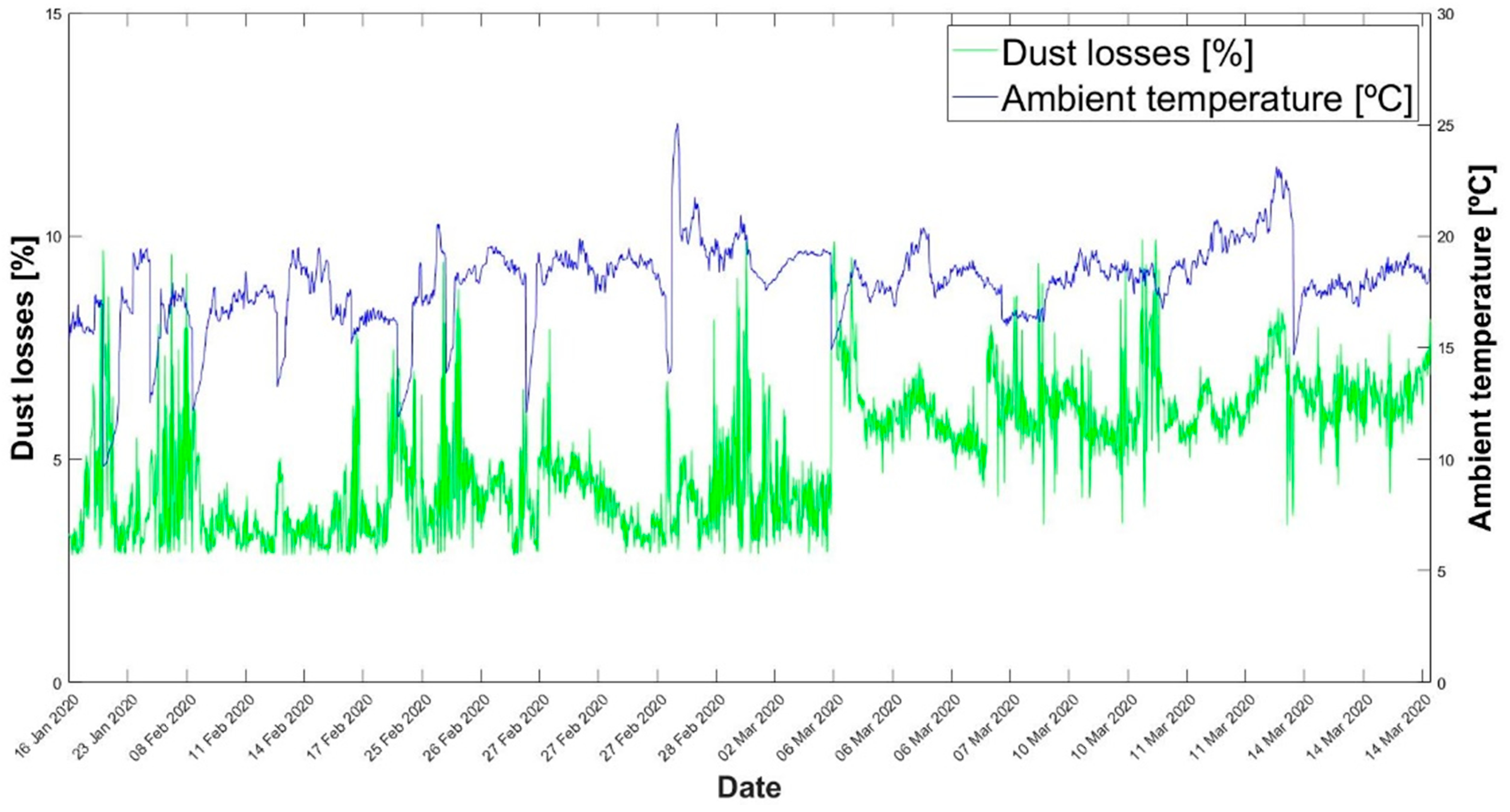
Figure 9 shows the dust losses (primary
y-axis) and the ambient temperature (secondary
y-axis) in function of time (
x-axis). There are probably areas where a common pattern can be seen in the two curves, and one can deduce that there may be some synchronicity between the ambient temperature and the dust loss. Above all, this will occur based on the time of day, so the irradiance in the array plane is probably also representative.
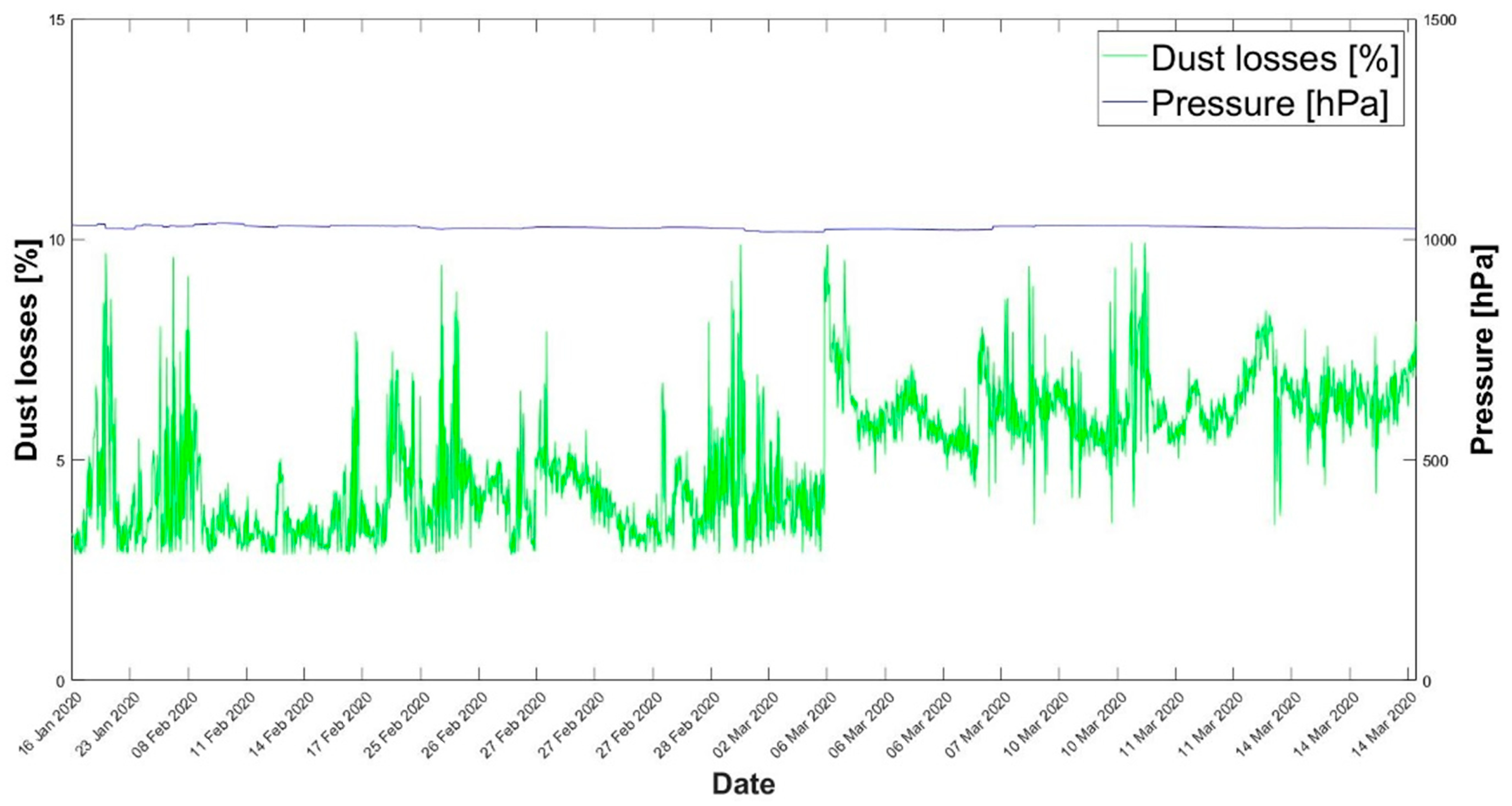
Figure 10 compares the dust losses (primary
y-axis) and the pressure (secondary
y-axis) in function of time (
x-axis). Pressure is a characteristic site variable that does not change over time so a clear relationship between the two variables cannot be established.
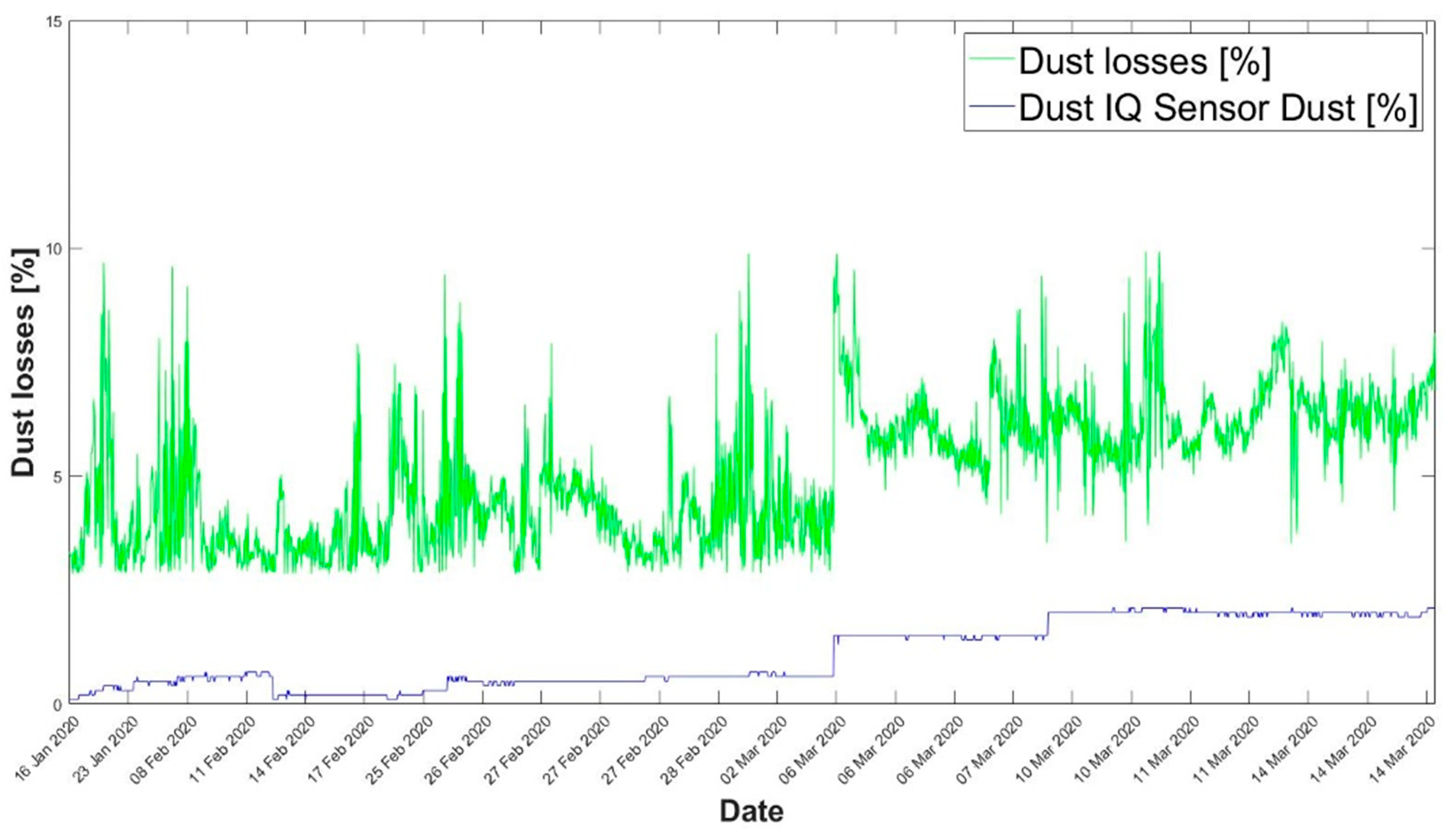
Figure 11 shows the variation in accumulated dust recorded by the experimental facility’s dust sensor (Dust IQ) and the dust losses determined according to the methodology set out in this work.
When representing both variables, it can be seen that significant differences in the magnitude of the sensor measurements are maintained. However, one can observe a similar trend to that in the losses determined.
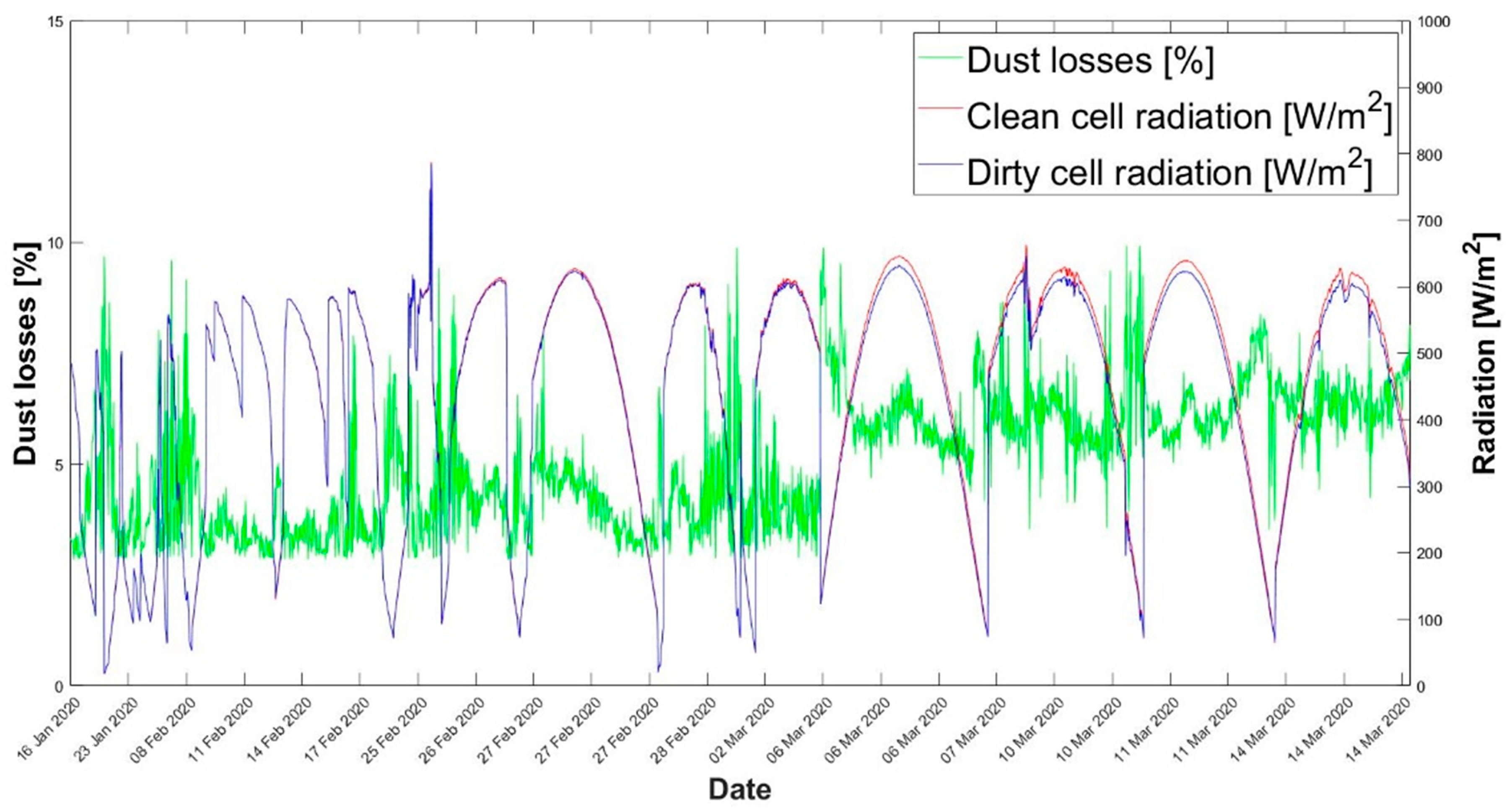
Figure 12 shows the variation in the dust losses determined (primary
y-axis) and the radiation of the calibrated cell when maintenance is carried out (secondary
y-axis). This graph demonstrates that which has previously been commented on: that the reduced production factor determination is more precise on clear days.
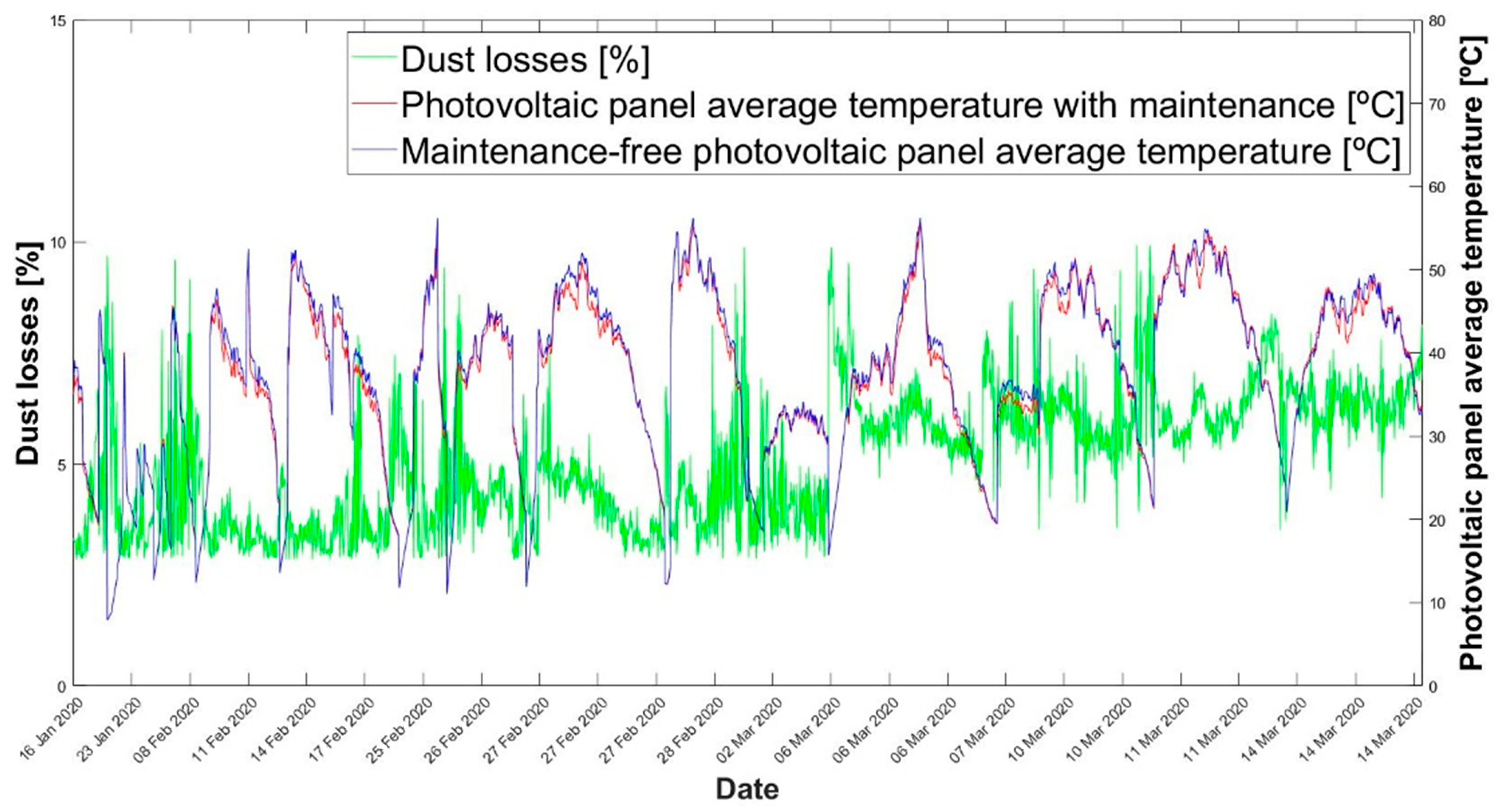
Finally,
Figure 13 shows the dust losses (primary
y-axis) and the average temperature determined for each panel based on the data provided by the resistive sensors installed in each panel (secondary
y-axis) against time (
x-axis).
As can be seen, the average temperature of the PV panel that received no maintenance was higher than that for the PV panel that did receive maintenance. This may be due to the generation of small hot spots caused by the non-uniform incidence of radiation on the panel with accumulated dust.
3.3. Solar Energy Research Center (CIESOL) Plant Simulation (9 kWp)
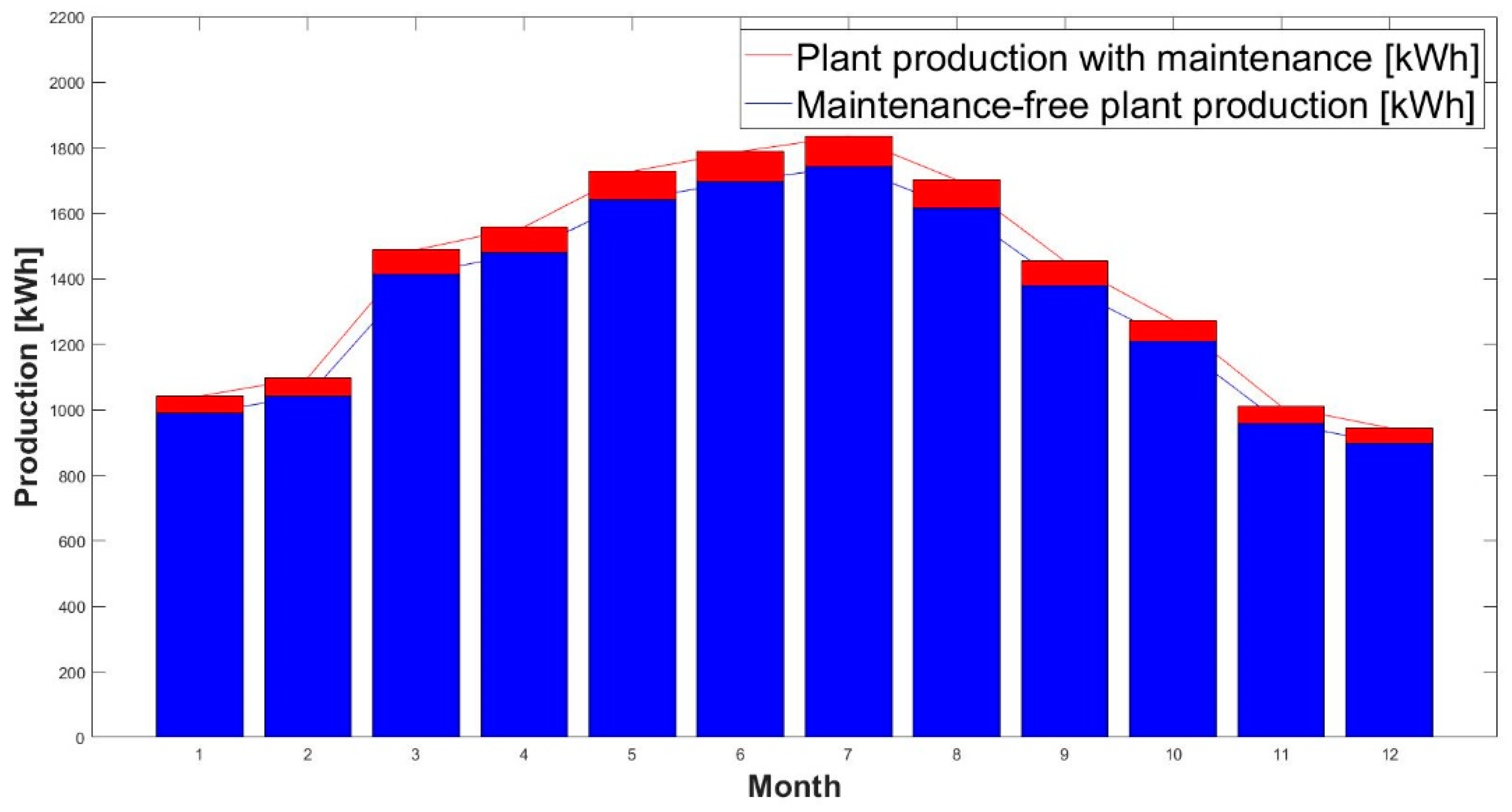
Figure 14 shows the results obtained when simulating the 9 kWp CIESOL plant in the two scenarios proposed in this paper. The monthly output, without taking into account the dust losses of the CIESOL plant in SAM, is shown in red. In blue, the resulting production is shown if the average reduced production factor from dust (calculated in the measurement campaign) were applied. In this case, the difference in production between the two proposed scenarios is not significant.
Based on the results obtained for both scenarios, and with the average monthly values for electricity sales in 2019, the revenues from each scenario are shown in
Table 5, where clean and dirty plant production [kWh] shown in the previous figure are presented in the form of columns (2nd and 3rd). The subsequent columns represent the product between the plant production and the average price of the electricity (
Table 2) and the final column is the difference between incomes of the clean and dirty plants.
This table breaks down the plant’s production for each of the implemented scenarios along with the monthly revenues generated in each. Additionally, the economic losses that would occur in each month if the plant were not cleaned have been broken down.
The last row summarizes the plant’s income under the different scenarios proposed and the total annual economic loss, which would amount to 41.06€. Hence, the annual economic loss in this case is practically irrelevant.
Figure 15 shows the approximate daily variation in dust losses that would be experienced by a plant in Rumah if it were in an optimally clean condition at the beginning of the year.
It can be seen that, in this region, the percentage of losses due to dust peaks in April, reaching 15%. Its lowest accumulated dust value occurs around July.
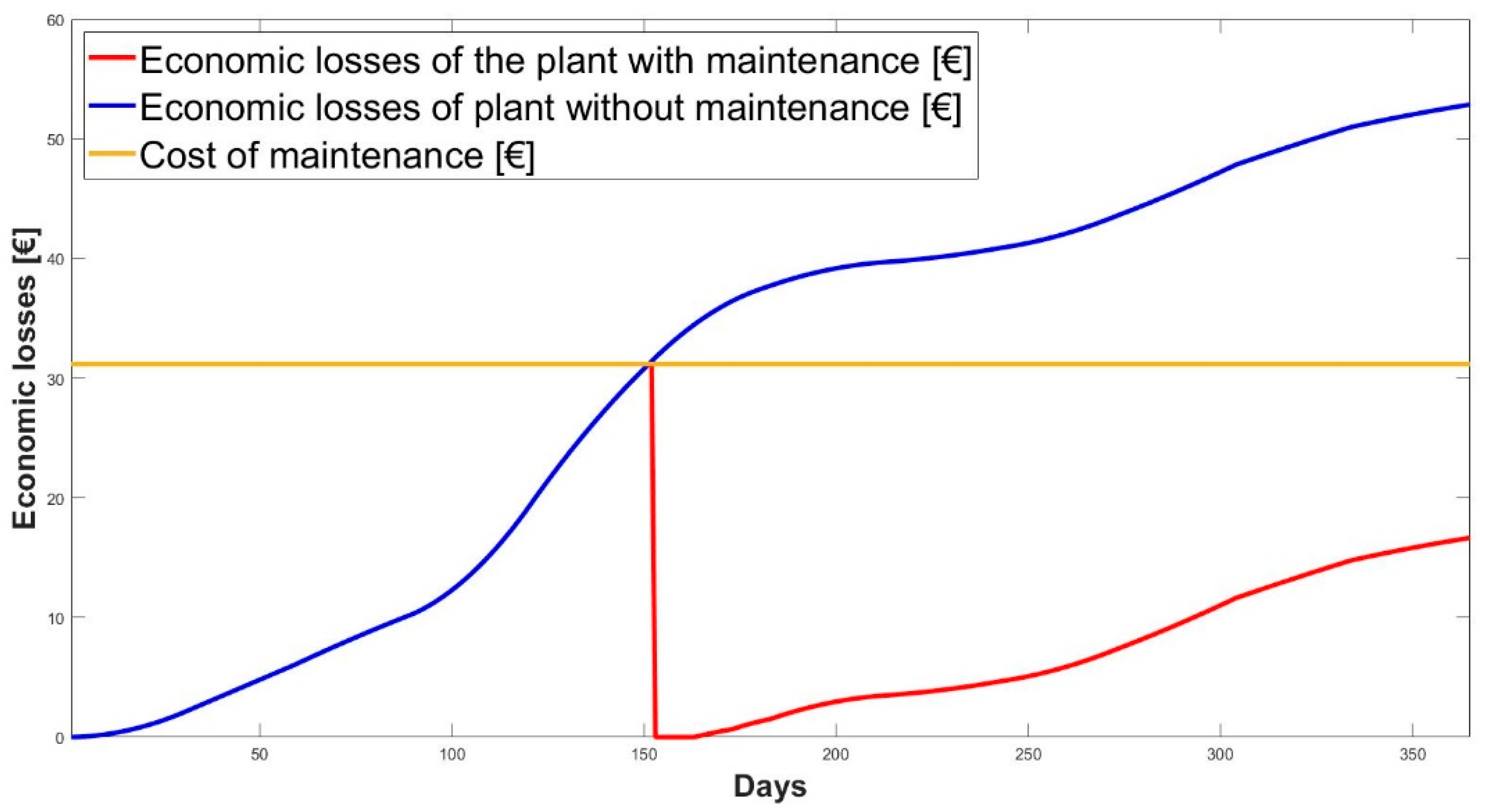
Figure 16 shows the accumulated economic losses for a year with and without maintenance if the production of the CIESOL plant and the losses due to dust recorded in Rumah are taken into account (
Figure 15), together with the maintenance cost of the CIESOL plant.
As the figure shows, if maintenance were carried out at this plant according to the methodology described above, it would be necessary to carry out a cleaning on the 152nd day (1 June), as this is the point at which the accumulated losses would exceed the plant cleaning cost.
Table 6 shows a breakdown of the losses that would occur in the plant with and without maintenance.
As shown in
Table 6, it would not be profitable to apply cleaning based on the methodology described above; this is because, at the end of the year, greater economic losses would be incurred than would be the case if regular maintenance were not carried out.
Maintenance would only be profitable if there were higher levels of contamination.
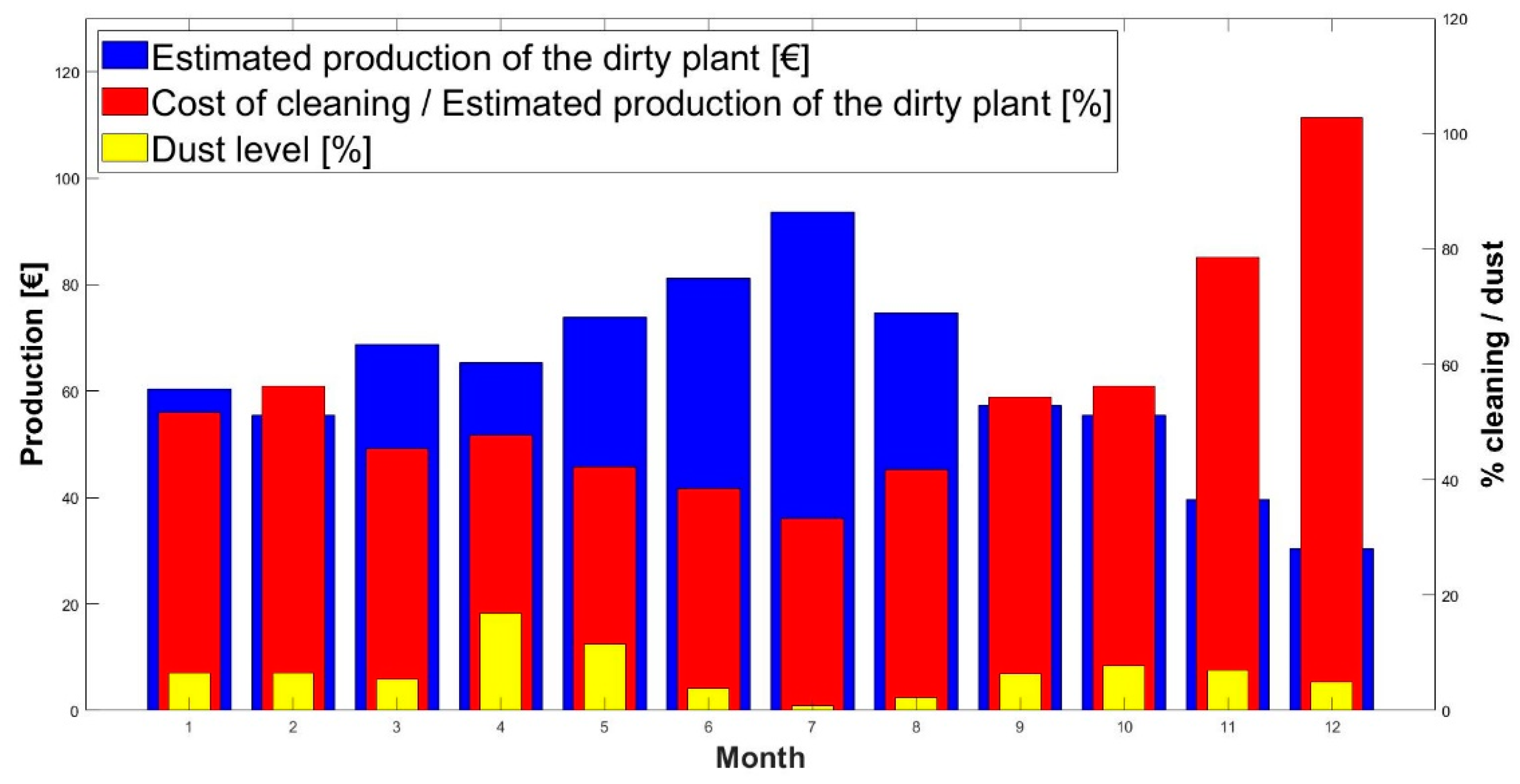
Figure 17 shows (in red) the dust level that would have to be reached each month for cleaning to be profitable, and the level of dust (in yellow) according to the methodology explained.
The red bars show the percentage of dust cleaning and the corresponding economic remuneration that would be obtained from the sale of the generated electricity (represented in blue).
To make cleaning profitable, the level of accumulated dust must exceed the proportion of economic remuneration that the cleaning corresponds to. As can be seen in the graph, the highest electricity sales values occur in the summer, so the proportion of cleaning costs is lower at that time. Plant cleaning will be more profitable during these months.
3.4. Simulation of the 1 MWp Plant
Figure 18 shows the monthly production of the 1 MWp plant simulation for the two scenarios presented in this paper.
As the monthly electricity generation at the photovoltaic plant increases, one can observe how the production losses associated with dust pollution become more important, arriving at losses of up to 10 MWh during the months of greatest generation.
Based on the results obtained for the two proposed scenarios, the values in
Table 7 are obtained.
In this industrial plant simulation, one can see how the economic losses associated with dust pollution during the months of greatest production amount to 460€. For this plant, the decrease in production due to dust translates into annual losses of 4466.85€, a considerable amount of money.
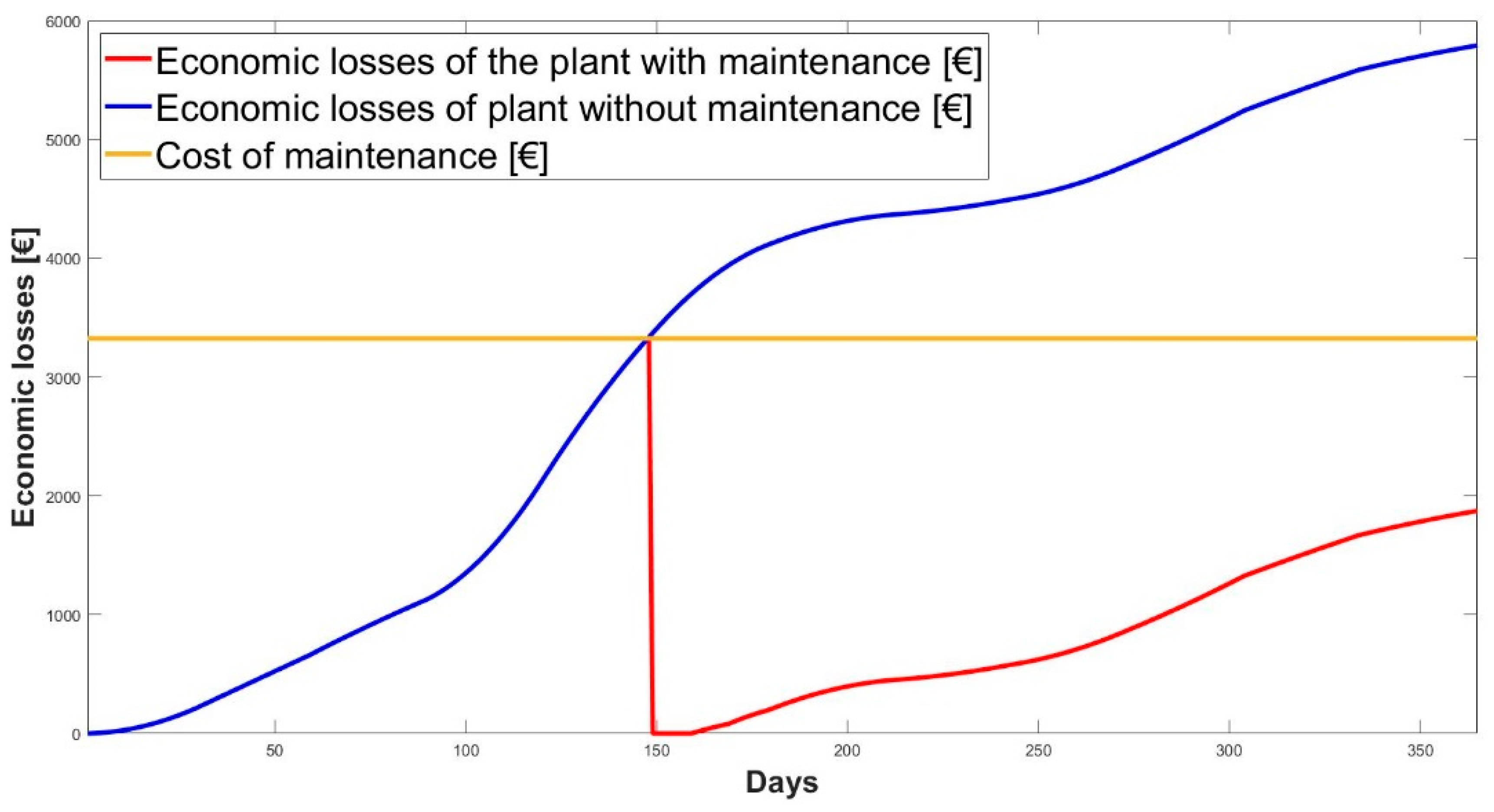
Figure 19 shows the accumulated economic losses over one year, with and without maintenance, together with the maintenance cost of the 1 MWp plant.
If maintenance were carried out at this plant in accordance with the above methodology, it would be necessary to clean it on day 148 (28 May) since this is the point at which the accumulated losses would be greater than the 3326€ that it would cost to clean the plant.
Table 8 shows a breakdown of the losses that would be incurred in the plant, with and without maintenance.
As in the case of the CIESOL plant, it would not be profitable to clean based on the methodology set out above, since the total economic losses would amount to 2745€ over the year if the cleaning work were carried out on the scheduled day.
In order for the investment involved in plant cleaning to be profitable, higher dust percentages would have to be present. The percentages of dust required to amortize the economic losses that would result from cleaning the plant are shown (in red) in
Figure 20.
One can observe how, in the summer months, the proportion of the cleaning cost in relation to the electricity sales would be greater. However, according to the data on the dust level used, in March the difference between this and the level that would be needed to make it profitable is less; that is to say, according to the data on the reduced production due to dust, it would be more profitable to clean in March as the difference would be smaller.
3.5. Simulation of the 50 MWp Plant
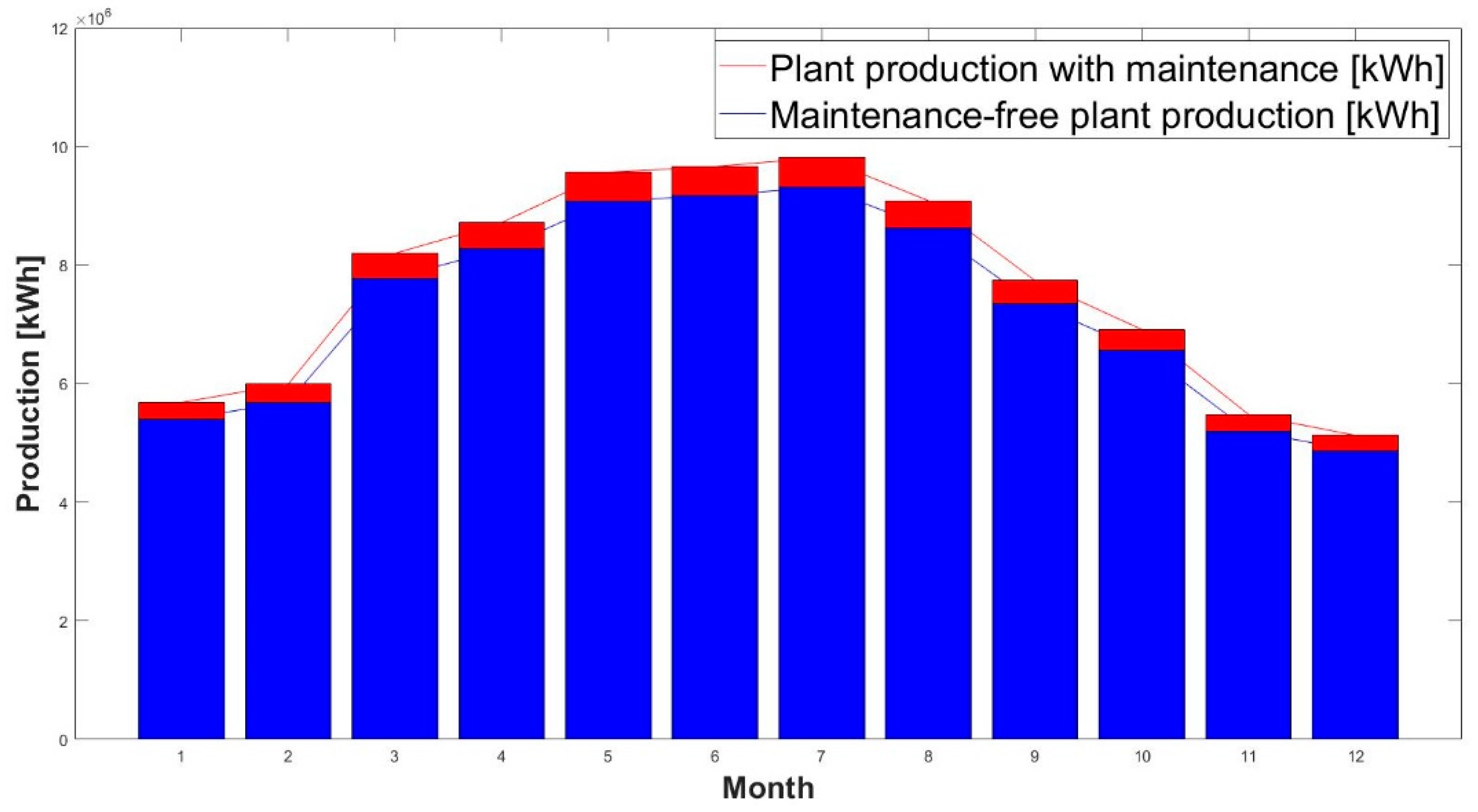
Figure 21 shows the results obtained for the 50 MWp plant for the two scenarios proposed. One can see how the difference in generation between the two scenarios is more notable in the months of greatest production. In this period, monthly production losses of up to 500 MWh would occur.
Table 9 presents the values based on the data obtained for both scenarios.
As one can observe, the economic losses associated with dust pollution for a 50 MWp plant would reach 25,000€ in the months of greatest production. The average soiling observed in the experimental plant would translate to annual losses of 223,342.68€ in a 50 MWp industrial plant.
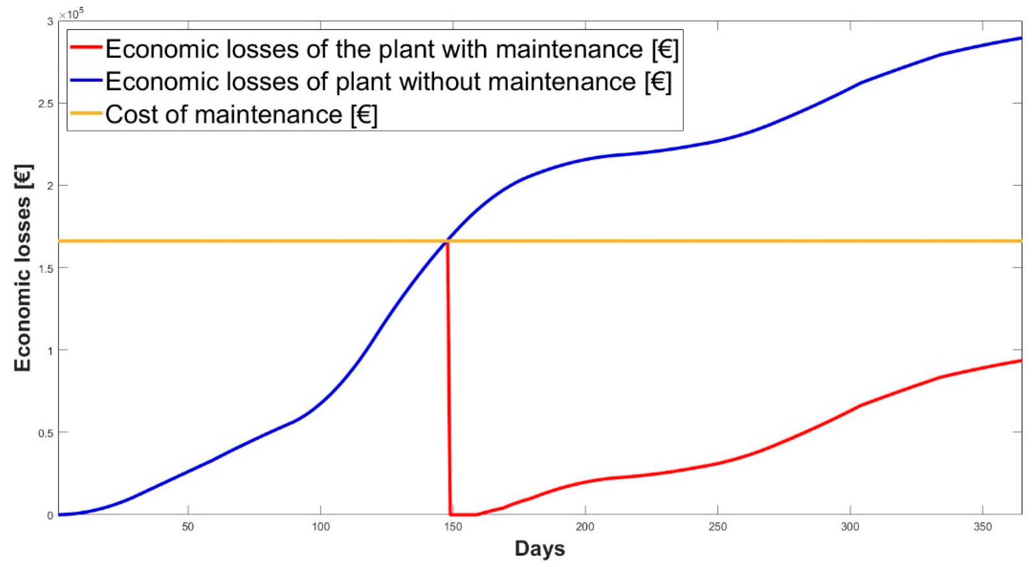
Figure 22 shows the graphical results of representing the accumulated economic losses over one year, with and without maintenance, together with the maintenance cost of the 50 MWp plant.
As can be seen, if maintenance were carried out at this plant in accordance with the methodology described above, it would be necessary to clean on day 148 (28 May), at which time the accumulated economic losses associated with dust contamination would exceed the plant’s cleaning cost, which amounts to 166,300€.
Table 10 gives a breakdown of the economic losses that would occur in the 50 MWp plant, with and without maintenance.
The cost of cleaning is still too high so cleaning would not be profitable as the total economic losses would amount to 137,330€; this economic loss is more than if the photovoltaic plant were not cleaned.
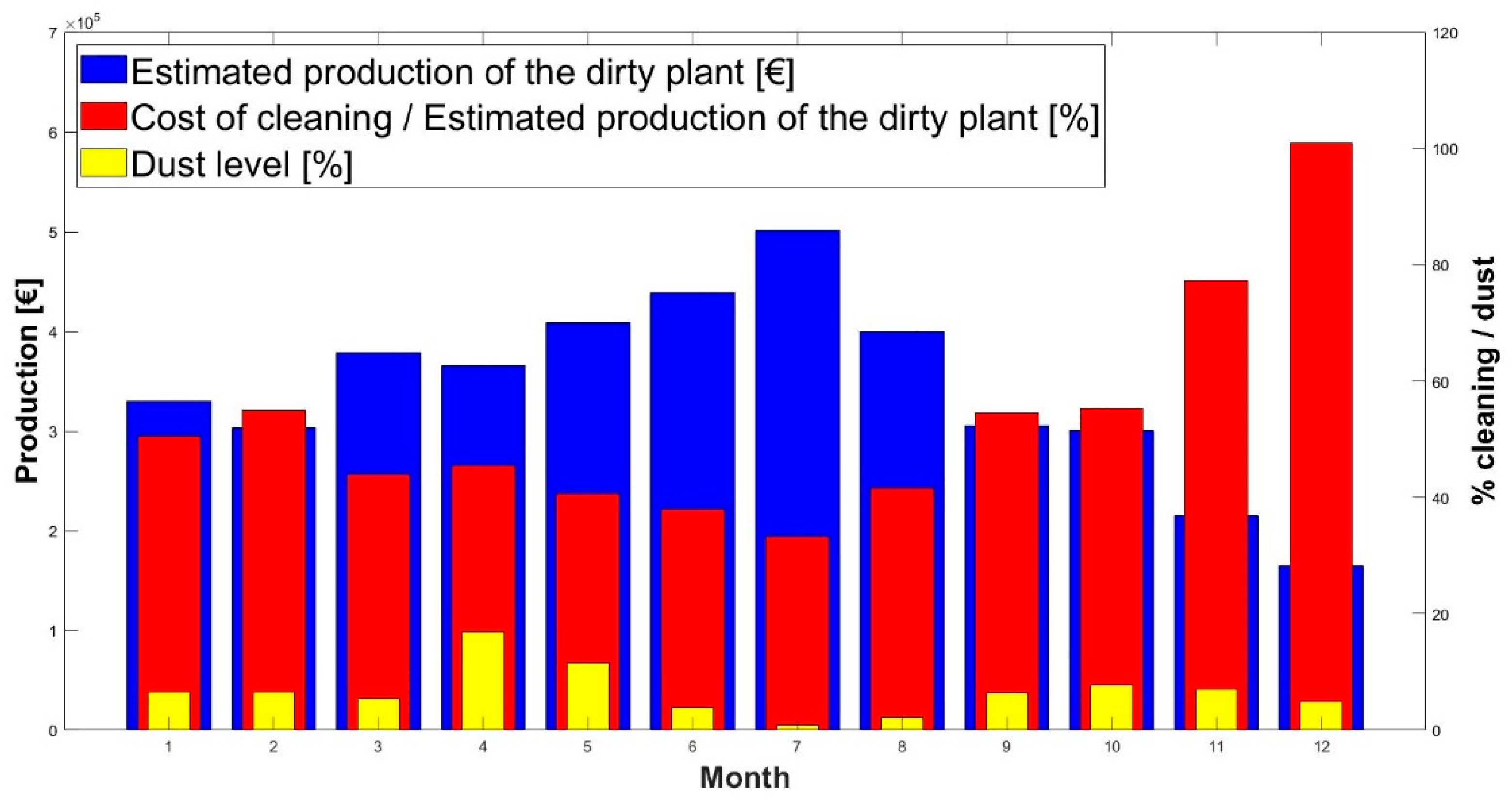
To achieve a return on the cleaning investment for a plant of this size, contamination levels equal to those described by the red bars in
Figure 23 would need to be reached.

 ,
, 


