Article

PV Power Prediction, Using CNN-LSTM Hybrid Neural Network Model. Case of Study: Temixco-Morelos, México

Energy Systems Department, Instituto de Energías Renovables, Universidad Nacional Autónoma de México, Priv. Xochicalco S/N Temixco, Morelos 62580, Mexico
*
Author to whom correspondence should be addressed.
Energies 2020, 13(24), 6512; https://doi.org/10.3390/en13246512
Submission received: 21 October 2020 / Revised: 3 December 2020 / Accepted: 5 December 2020 / Published: 10 December 2020
(This article belongs to the Special Issue Model Predictive Control for Energy Management in Microgrids)

Abstract

:
Due to the intermittent nature of solar energy, accurate photovoltaic power predictions are very important for energy integration into existing energy systems. The evolution of deep learning has also opened the possibility to apply neural network models to predict time series, achieving excellent results. In this paper, a five layer CNN-LSTM model is proposed for photovoltaic power predictions using real data from a location in Temixco, Morelos in Mexico. In the proposed hybrid model, the convolutional layer acts like a filter, extracting local features of the data; then the temporal features are extracted by the long short-term memory network. Finally, the performance of the hybrid model with five layers is compared with a single model (a single LSTM), a CNN-LSTM hybrid model with two layers and two well known popular benchmarks. The results also shows that the hybrid neural network model has better prediction effect than the two layer hybrid model, the single prediction model, the Lasso regression or the Ridge regression.

1. Introduction

Nowadays renewable energy (RE) aims to be a real solution to solve the fossil fuel problem. A very well known renewable energy is solar photo-voltaic (PV), which is also in fast growth. Global PV capacity is estimated to increase significantly from 593.9 GW in 2019 to 1582.9 GW in 2030 following significant capacity additions by China, India, Germany, the US and Japan [1]. Solar PV generation plays an important role in the future of energy structure. According to some estimations of the Joint Research Centre (JRC), solar PV power generation capacity may reach 1.4 TW by 2024 just in Europe [2]. Nevertheless, the intermittent nature of the solar resource poses big challenges for energy integration into existing energy systems. Precise PV prediction is a good way to solve this problem [3].
On the other hand, over the past eight years, off-grid systems in the form of stand-alone solar home systems (SHS’s) have proved the most popular and immediate solution for increasing energy access in rural areas across the Global South [4]. In Mexico, there are aprox. 1.2 million people living without access to the electrical grid [5]. SHS’s can be a real option to empower rural communities with autonomous energy production [6]. In rural places with solar resource and with no access to the grid, this is a viable solution.
The interconnection of existing stand-alone solar home systems can form micro grids [4]. This tiny grid is formed by prosumers (households capable of producing and consuming electrical power, Figure 1) and consumers (households only consuming power). In this new architecture of distributed PV generation, many authors propose that consumers and prosumers can even trade self-produced energy on a micro grid energy market. This involves an information layer that feeds data to an energy management system (EMS) as it is shown in Figure 1. The EMS acts as the middleman between the physical and the information layer. The EMS needs to have accurate prediction photo voltaic power (PVP) models, consumption prediction models, an energy market model and other tools which are essential in a smart energy management system for increasing reliability, sustainability, efficiency and flexibility [7,8,9,10].
In general, there are three main prediction methods: statistical models, physical models and machine learning models. The physical model relies on dynamics between solar radiation and laws of physics [11]. The statistical model mainly depends on historical data, statistics and probability theory to forecast future time series [12,13]. The machine learning models map directly from inputs to outputs, they extract complex nonlinear features in a very efficient way [14,15]. In the machine learning models we can highlight artificial neural networks (ANN) especially one type of ANN. Recurrent neural networks (RNN), which is one of the most commonly used methods for forecasting time series [16,17]. The RNN has been studied in various applications like wind speed prediction [18], energy power consumption prediction [19,20] or even traffic prediction [21], achieving excellent results.
However, one common problem in RNN (with gradient-based learning methods and back-propagation), is the vanishing of gradient. Gradient vanishing occurs while training long data sequences. This means that the gradient of the loss function approaches zero, making the network hard to train [22]. Long Short Term Memory networks (LSTM) solve this problem [23,24].
PV prediction using LSTM models has been studied by many authors [14,17,22] achieving to reduce the prediction error compared with other traditional methods.
In recent years, many researchers have combined CNN and LSTM models to extract temporal and spacial features. In the medical field Gill et al. proposed a CNN-LSTM model to accurately detect arrhythmias in the ECG [16]. Zhang C. Y. used deep belief networks (DBN) for wind speed prediction [21] achieving better results than the traditional methods (such as SVR). Kim [25] proposed a hybrid CNN-LSTM model for electric energy consumption achieving superior results than other deep learning based methods. They found that extracting first the local features and then temporal ones worked better than a LSTM-CNN model, performing with a medium square error (MSE) of 3.738. They also found that time series decomposition with deep learning models provides useful visualizations to better understand the problem of predicting and analyzing energy consumption.
Wang et al. proposed an hybrid LSTM-CNN model for PV power prediction [26]. Accomplishing four main contributions:
  • They proposed a hybrid photo voltaic power prediction deep learning model which considers the temporal and local features.
  • The temporal features of the data were first extracted (using a LSTM model) and then the local features using a CNN model.
  • They reduced the complexity of the model by selecting the 1D-CNN model to extract the local features, and then the data conversion link was eliminated. Therefore PV power prediction is greatly facilitated.
  • They compared with other models (CNN, LSTM, CNN-LSTM), to prove the validity of the model.
Wang et al. [26] proposed a hybrid model of one dimension for PV prediction. In this work we choose a hybrid model with a stronger multi-layer architecture, this includes a 5D-CNN model with max pooling and a 5D-LSTM model. Indeed, the five dimensional CNN and LSTM model will consume more computational resources for training than a uni-dimentional model, but high accuracy will be achieved [27,28]. Therefore, the computational time and some metrics such as the mean square error (MSE) of the proposed model will be compared with other deep learning models.

2. The Dataset

We use data of a 1.7 kW photo voltaic solar system (PVSS) and from a meteorological station (the ESOLMET station (Figure 2)) 120 m from the PVSS (Figure 3), in the IER-UNAM (Renewable Energy Institute) in Temixco, Morelos, México. Latitude: 18°50′25.62′′ N, longitude: 99°14′10.49′′ W at 1253 m above sea level.
The electric variables measured from the PVSS after the inverter are the following: active power generated [W], average phase current generated [A] and the AC Voltage generated [V]. The variables available by the ESOLMET are: direct radiation [W/m2], global radiation [W/m2], diffuse radiation [W/m2], temperature [°C], humidity [%], wind speed [m/s] and barometric pressure [mBar]. All these ten variables will conform our dataset, and are shown in Figure 4.
The dataset consists of 52,428 values per variable. From the date: 01/01/2019 00:00:00:00 to the date: 01/01/2020 00:00:00:00, with a resolution of 10 minutes. We used 80% of the data to train the model (41,942 values) and 20% to validate our predictions(10,486 values).
Photo voltaic power generated (PVPG), is the variable we want to predict, in Figure 5. PVPG is shown through the complete year. As it will be explained in detail in the next section, our model takes an input of 10 variables and the proposed neural network throws a specific output(PVPG) in time.

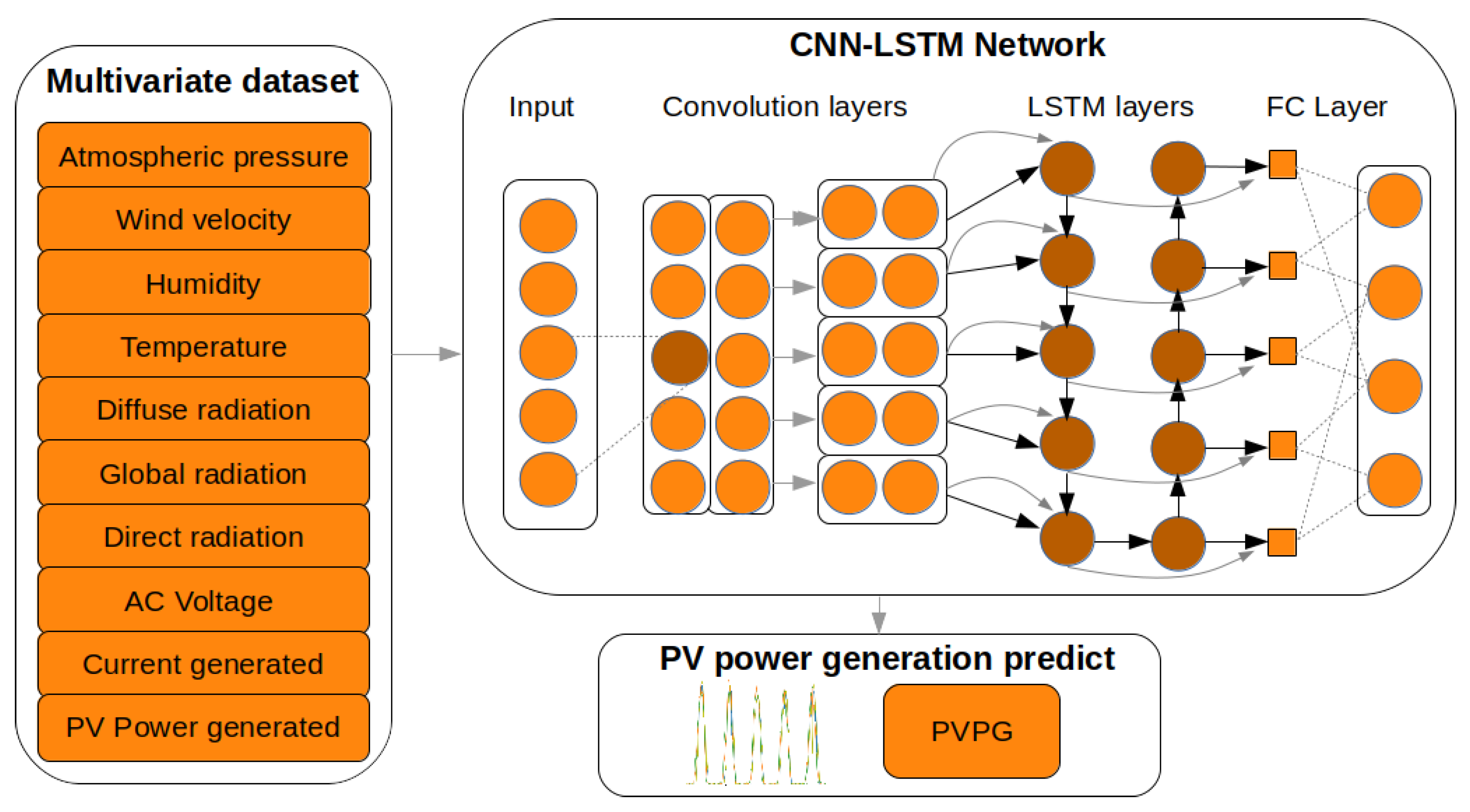
3. Proposed Hybrid Model

3.1. Local Feature Learning with CNN

CNN are very popular for extracting local features in images, for example. Convolution is the main concept of a CNN. Our proposed CNN includes two parts: the convolutional layers (Equations (1) and (2)) and the pooling layer (the main purpose of this layer is to reduce the number of parameters of the tensor by reducing its size Figure 6) which helps to reduce computation time.
In the convolution layer, the previous layer features graph interacts with the convolutional kernel; this interaction forms the output feature graph j of the convolutional layer. Each one of this output feature graph j might contain a convolution with multiple input feature graphs.
The equations that define the convolution layer are:
y j ( l ) = ( i c j t i l 1 w i j ( l ) ) + b j ( l )
where c j is a set of input feature graphs. b j l is the bias, y j l the output of the convolution and w i j ( l ) the convolution kernel.
t j l = f ( y j ( l ) )
t j l the feature graph of the convolution layer l.
f ( x ) = m a x ( 0 , x )
f is known as the activation function. In this work we use a rectified linear unit (Relu) defined in Equation (3).

3.2. Temporal Feature Learning with LSTM

The lower layers of the proposed model are the LSTM. This layers store time information about important characteristics of PV power generation extracted by the CNN. LSTM preserves long-term memory by using memory units that can update the previous hidden state. This functionality makes it possible to understand temporal relationships on a long-term sequence. This time recurrent neural network was proposed by Hochreiter & Schmidhuber in 1997 [30]. Its internal memory unit and gate mechanism overcome the gradient disappearance problem that occurs in training traditional recurrent neural networks (RNN). The memory channel and the gate mechanism (which includes: forget gate, input gate, update gate and output gate) are shown on Figure 7. The equations of the LSTM model are the following [24]:
f t = σ ( W f [ h t 1 , X t ] + b f )
f t is the output value of the forget gate. And σ refers to the sigmoid activation function.
i t = σ ( W i [ h t 1 , X t ] + b i )
i t is the output value of the input gate.
g t = t a n h ( W g [ h t 1 , X t ] + b g )
g t is the output value of the update gate.
c t = f t c t 1 + i t g t
c t refers to the memory cell.
o t = σ ( W o [ h t 1 , X t ] + b o )
o t is the output value of the output gate.
h t = o t t a n h ( c t )
where h t is the output vector result of the memory cell at time t (see Figure 2). W f , i , g , o are the weights matrices and b f , i , g , o the bias vectors.
Figure 7. LSTM cell.
Energies 13 06512 g007

3.3. CNN-LSTM Hybrid Model

The proposed CNN-LSTM structure as it is shown in Figure 8. consists of a five CNN and LSTM layers and a full connected layer. The input of the neural network has ten variables, such as temperature, irradiance, global radiation and others (see the section Dataset for more information about the variables).
First, the upper layer of CNN-LSTM consists of CNN. The CNN layer can receive various variables that affect PV power generated, such as voltage, intensity, and global radiation. On the other side, the dataset is separated in two parts: 80% for training the model and 20% to validate the results. In the validation part we used PVPG in Temixco during 2019 as shown on Figure 5.
The CNN consists of an input layer that accepts sensor variables as inputs, an output layer that extracts features to LSTMs, and several hidden layers. The hidden layers used consists of: a convolution layer, a ReLU layer, an activation function, or a pooling layer.
From the presented data in the input a unique output pattern is generated. The CNN extracts the local features and the LSTM temporal part. With this structure, the neural network “learns” for every input a weight that determines a specific output.
The CNN configuration in the hybrid model mainly consists of five convolutional layers and five pooling layers. The number of convolution kernels is 64, 128, 256, 128 and 64 respectively with a ReLU activation function.
The LSTM model in the hybrid model contains five hidden layers, having respectively 64, 128, 256, 128 and 64 neurons. Finally, there is a dropout of 0.1 to prevent overfitting and finally two fully-connected layers with 2048 and 1024 neurons respectively. For this experiment 1000 epochs were selected. The specific parameter settings of the model are shown in the following Table 1.
All the hyper-parameters were designed by the trial and error method. This process means that certain hyper-parameters are specified, then trained with 80% of the data and validated with other 20%, for the four seasons throughout the year. Hyper-parameters are then changed and the process is repeated until they are finally optimized.
In order to demonstrate the good performance of the proposed model, the results obtained by our model are compared with other models (LSTM and 2D CNN-LSTM) and two well known benchmarks [31]. We will forecast PVPG for three different scenarios: summer, fall and winter. These results will be further discussed in the last sections.

4. Performance Evaluation Metrics

For this work, we selected some metrics to evaluate the model. They are: MSE (Mean Square Error), RMSE (Root Mean Square Error) and MAE (Mean Absolute Error). These metrics are defined as follows [25]:
M S E = 1 n i = 1 n ( Y i Y ^ i ) 2
R M S E = 1 n i = 1 n ( Y i Y ^ i ) 2
M A E = i = 1 n Y i Y ^ i n
where: Y i is the real PVPG value, Y ^ i the predicted value and n the number of Y i .
MSE, RMSE and MAE have been used as a standard statistical metric to measure models performance. This is an easily computable quantity because is sample-dependent [32,33].

5. Results

5.1. Performance Comparison with Other Deep Learning Models

In this work we propose a five CNN layer with max-pooling, a five layer LSTM structure and a fully connected layer, also known as dense layer. We used the framework Keras and Tensorflow in Python 3.6 to program the models. The computational process was accomplished in a personal computer, with a 64 bit operating system, 8 GB of RAM with an Intel Core processor i7-4700MQ (2.4 GHz, 6 MB cache and 4 cores).
A part of the dataset was used to train the model (80 %) and another part was used to verify the predictions (20 %). Figure 9, Figure 10 and Figure 11 show the graphs of the PV power prediction during summer, fall and winter respectively. On the X axis, we have time with a 10-min time resolution and on the Y axis, power in [W]. The blue curve are the actual measurements and the yellow curve is the prediction of the five-layer hybrid model, the orange curve corresponds to the two-layer model and the green curve is a five-layer LSTM model.
The metrics that evaluate the performance of the different models are shown in Table 2. In Table 3, the computation time processing for each model is displayed (Time window prediction is of 10 min for this experiment).
As it is shown in Figure 10, Figure 11 and Figure 12, if we compare the single LSTM and the 2D CNN-LSTM models with the five layer CNN-LSTM model we can observe that the five layer model can predict more efficiently irregularities in Figure 13 is accomplished with a strong 5D CNN-LSTM network.
It is observed that the lowest MSE (0.0068) corresponds to the most robust five-layer model (5D CNN-LSTM) This model also has the biggest time processing of almost 70 s.
On the other hand, the 5D-LSTM model and the 2D CNN-LSTM model obtained a very similar RMSE (0.2923 and 0.2429 respectively). The same with the MAE, 0.1666 for the LSTM model, 0.1410 for the 2D CNN-LSTM model and 0.0519 for the 5D CNN-LSTM model.

5.2. Performance Comparison with Competitive Benchmarks

We compare the performance of the proposed method with competitive benchmarks using Temixco ESOLMET dataset [34]. Table 4 summarizes the performance of competitive benchmarks (Time window prediction is of 10 min for this experiment.).
Yang et al. refer to benchmarking, a essential practice in solar prediction for comparing published results [35]; some authors like Pedro et al., used some well known benchmarks based on linear regression: Lasso and Ridge regression [31]. We select these two models for benchmarking due to their high interpretability and availability in statistical software and in Python.
Furthermore, we compare competitive benchmarks with the proposed model, the results are shown in Table 4. The forecasting horizons range from 10-min ahead to 180-min ahead. As it is expected, when the horizon prediction increases the RMSE also does it in a linear way (Figure 13).
It can be seen that the proposed model can provide good prediction performance. Moreover, at all prediction horizons in the study cases, the proposed method has the smallest RMSE metrics, which shows the best prediction performance compared to other competitive benchmarks.
Most of the related work [26,36,37,38], uses a single layer approach for PV power prediction. Nevertheless, the results of this work show metrics like MSE, to be ten times lower for a multi-layer CNN-LSTM deep neural architecture. This obviously comes with more processing time for training the model, as it is shown in Table 3. However, this time is completely useful for all of the prediction horizons presented, and can be dropped down if the model is trained with a GPU or TPU processing unit.
Also results for different prediction horizons (from 10-min horizon to 180-min horizon) show the RMSE of the proposed model to be lower than competitive benchmarks in all cases (see Table 4 and Figure 13).

6. Conclusions

We use real data from the location 18°50′24.1′′ N 99°14′09.0′′ W (Temixco, Mexico) to train and validate a 5D CNN-LSTM hydrid model. The dataset was composed by ten variables such as temperature, solar radiation and others, for predicting PV power generation (PVPG). A five layer CNN-LSTM hybrid model was compared with a single LSTM model and another CNN-LSTM hybrid model of two layers. The error of a robust CNN-LSTM net (in this experiment with five layers) was: M S E = 0.00689 , as shown in Table 2. Therefore, we can say that there is a considerable correlation between a robust neural network model with a highly accurate prediction effect.
We propose a CNN-LSTM model for precise prediction of PV power energy generation. The 5D CNN-LSTM hybrid model accurately predicts PV power generation by extracting features from variables that affect PVPG. The proposed model is compared to other machine learning methods to demonstrate its usefulness. We used CNN-LSTM to learn trends in the PVPG and temporal information from multivariate time-series.
The CNN-LSTM model proposed in this paper predicts irregularities in PV power generation (PVPG) that could not be well learned by other existing machine learning models. In Figure 13 we see how on a rainy day the 5D CNN-LSTM model (in green) is exact by predicting the irregular PVPG trend in cloudy conditions.
The results of this paper represent that the 5D CNN-LSTM model predicts PVPG with high accuracy, and shows the highest performance compared with the single LSTM model and the 2D CNN-LSTM hybrid model. The results also shows the highest performance compared with two existing competitive benchmarks.
Nevertheless, the computational time for a five layer hybrid model (69.1148 s) is bigger than the two layer hybrid model (8.0362 s) or the single LSTM model (5.1394 s) as it is shown in Table 3. A neural network prediction model should take in consideration that a high accuracy performance is compromised by computational time processing.
On the other hand, the introduction of TPU’s (Tensor Processing Units) had include hardware advantages with faster computational processing time [39], this experiments were conducted in a CPU Intel Core i7, but robust hybrid neural networks models like the one presented in this work, should be studied in new generation hardware like the Coral TPU accelerator introduced by Google [40], in order to reduce time processing and increase performance.
Also, further studies should be done to implement dynamic prediction systems (generation and consumption in households) with data available from an IoT network of devices in low cost and low power in open-source platforms. Thus, aiming to create tools for a smart grid and efficient trading energy management systems.

7. Future Work

The proposed model will be integrated in a Raspberry Pi 3 with a Coral TPU accelerator to have a real time data prediction system. The general scheme is shown in Figure 14. The ESP32 sends measurements to an IoT server (Thingsboard). This real time data is also available for the Raspberry Pi to calculate new weights and update the hybrid model. The Coral TPU will provide the Raspberry Pi the capability to run machine learning models. This kind of low cost system will be possible to use in multiple prosumers in a micro-grid environment.
Accurate PV power and electric energy consumption predictions are essential for energy management systems in energy transaction architectures [8,41,42,43], where energy becomes a medium of exchange. A low power prediction processing unit such as a Raspberry can increase the performance of SHS’s in rural areas by introducing a trading energy prediction mechanism but more studies should be done in this area.

Author Contributions

Conceptualization, M.R. and M.T.; methodology, M.R.; software, M.T. and F.R.; validation, M.T.; formal analysis, M.T.; investigation, M.T.; resources, M.R.; data curation, M.T.; writing—original draft preparation, M.T.; writing—review and editing, M.T.; visualization, M.T.; supervision, M.R.; project administration, M.R.; funding acquisition, M.R. All authors have read and agreed to the published version of the manuscript.

Funding

This research received no external funding.

Acknowledgments

This work was supported by the National Council of Science and Technology of México (CONACYT) and the equipment of the Renewable Energy Institute of the National University of Mexico (IER—UNAM).

Conflicts of Interest

The authors declare no conflict of interest.

Abbreviations

The following abbreviations are used in this manuscript:
RERenewable energy
CNNConvolutional neural network
1D-CNNOne dimension convolutional neural network
5D-CNNFive dimension convolutional neural network
LSTMLong short term memory
ReLURectified Liniar Unit
PVPhoto voltaic
PVPGPhoto voltaic power generated
PVSSPhoto voltaic solar system
SHSSolar home system
JRCJoint Research Centre
ANNArtificial neural network
RNNRecurrent neural network
DRNDeep belief network
EMSEnergy management system
SVRSupport Vector Regression
ECGElectrocardiogram
UNAMUniversidad Nacional Autónoma de México
IERInstituto de Energías Renovables
TPUTensor Processing Unit

References

  1. Data, G. Solar Photovoltaic (PV) Market, Update 2019—Global Market Size, Market Share, Average Price, Regulations, and Key Country Analysis to 2030; GlobalData: London, UK, 2019. [Google Scholar]
  2. Jaeger-Waldau, A. PV Status Report 2019, EUR 29938 EN; Publications Office of the European Union: Luxembourg, 2019. [Google Scholar]
  3. Sobri, S.; Koohi-kamali, S.; Rahim, N.A. Solar photovoltaic generation forecasting methods: A review Number of Day. Energy Convers. Manag. 2020, 156, 459–497. [Google Scholar] [CrossRef]
  4. Soltowski, B.; Campos-gaona, D.; Strachan, S.; Anaya-lara, O. Bottom-Up Electrification Introducing New Smart Grids Architecture—Concept Based on Feasibility Studies Conducted in Rwanda. Energies 2019, 12, 2439. [Google Scholar] [CrossRef] [Green Version]
  5. Inegi; Sener, C. Encuesta Nacional Sobre Consumo de Energéticos en Viviendas Particulares. ENCEVI, 2018 Consulted on June 2020. Available online: https://www.inegi.org.mx/contenidos/programas/encevi/2018/doc/encevi2018_presentacion_resultados.pdf (accessed on 10 June 2020).
  6. Bahaj, A.; Blunden, L.; Kanani, C.; James, P.; Kiva, I.; Matthews, Z.; Price, H.; Essendi, H.; Falkingham, J.; George, G. The Impact of an Electrical Mini-grid on the Development of a Rural Community in Kenya. Energies 2019, 12, 778. [Google Scholar] [CrossRef] [Green Version]
  7. Khorasany, M.; Donald Azuatalam, R.G.A.L.; Razzaghi, R. Transactive Energy Market for Energy Management in Microgrids: The Monash Microgrid Case Study. Energies 2020, 13, 2010. [Google Scholar] [CrossRef]
  8. Mengelkamp, E.; Kessler, S.; Gärttner, J.; Rock, K.; Orsini, L.; Weinhardt, C. Designing microgrid energy markets. Appl. Energy 2017, 210, 870–880. [Google Scholar] [CrossRef]
  9. El-baz, W.; Tzscheutschler, P.; Wagner, U. Integration of energy markets in microgrids: A double-sided auction with device-oriented bidding strategies. Appl. Energy 2019, 241, 625–639. [Google Scholar] [CrossRef]
  10. Bahrami, S.; Amini, M.H. A Decentralized Framework for Real-Time Energy Trading in Distribution Networks with Load and Generation Uncertainty. arXiv 2017, arXiv:1705.02575v1. [Google Scholar]
  11. Blaga, R.; Sabadus, A.; Stefu, N.; Dughir, C.; Paulescu, M. A current perspective on the accuracy of incoming solar energy forecasting. Prog. Energy Combust. Sci. 2019, 70, 119–144. [Google Scholar] [CrossRef]
  12. Haji, R.; Zargar, M.; Yaghmaee, M.H.; Member, S. Development of a Markov-Chain-Based Solar Generation Model for Smart Microgrid Energy Management System. IEEE Trans. Sustain. Energy 2020, 11, 736–745. [Google Scholar]
  13. Gao, M.; Wang, K.; Chain, A.C.T.M. Probabilistic Model Checking for Green Energy Router System in Energy Internet. In Proceedings of the GLOBECOM 2017—2017 IEEE Global Communications Conference, Singapore, 4–8 December 2017. [Google Scholar]
  14. Voyant, C.; Notton, G.; Kalogirou, S.; Nivet, M.L.; Paoli, C.; Motte, F.; Fouilloy, A. Machine learning methods for solar radiation forecasting: A review. Renew. Energy 2017, 105, 569–582. [Google Scholar] [CrossRef]
  15. Chandler, S.A.; Hughes, J.G. Smart Grid Distribution Prediction and Control Using Computational Intelligence. In Proceedings of the 2013 1st IEEE Conference on Technologies for Sustainability (SusTech), Portland, OR, USA, 1–2 August 2013; pp. 86–89. [Google Scholar]
  16. Gómez-Gil, P.; Ramírez-Cortes, J.M.; Pomares Hernández, S.E.; Alarcón-Aquino, V. A neural network scheme for long-term forecasting of chaotic time series. Neural Process. Lett. 2011, 33, 215–233. [Google Scholar] [CrossRef]
  17. Abdel-Nasser, M.; Mahmoud, K. Accurate photovoltaic power forecasting models using deep LSTM-RNN. Neural Comput. Appl. 2019, 31, 2727–2740. [Google Scholar] [CrossRef]
  18. Ba, Ü.; Filik, T. Wind Speed Prediction Using Artificial Neural Networks Based on Multiple Local Measurements in Eskisehir. Energy Procedia 2017, 107, 264–269. [Google Scholar]
  19. Le, T.; Vo, M.T.; Vo, B.; Hwang, E.; Rho, S. Improving Electric Energy Consumption Prediction. Appl. Sci. 2019, 9, 4237. [Google Scholar] [CrossRef] [Green Version]
  20. Muralitharan, K.; Sakthivel, R.; Vishnuvarthan, R. Neural Network based Optimization Approach for Energy Demand Prediction in Smart Grid AC PT US CR. Neurocomputing 2017. [Google Scholar] [CrossRef]
  21. Li, Y.; Yu, R.; Shahabi, C.; Liu, Y. Diffusion convolutional recurrent neural network: Data-driven traffic forecasting. In Proceedings of the 6th International Conference on Learning Representations, ICLR 2018—Conference Track Proceedings, Vancouver, BC, Canada, 30 April–3 May 2018; pp. 1–16. [Google Scholar]
  22. Al-Dahidi, S.; Ayadi, O.; Adeeb, J.; Alrbai, M.; Qawasmeh, B.R. Extreme Learning Machines for Solar Photovoltaic Power Predictions. Energies 2018, 11, 2725. [Google Scholar] [CrossRef] [Green Version]
  23. Tang, Q.; Yang, M. ST-LSTM: A Deep Learning Approach Combined Spatio-Temporal Features for Short-Term Forecast in Rail Transit. J. Adv. Transp. 2019, 2019, 8392592. [Google Scholar] [CrossRef] [Green Version]
  24. Madondo, M.; Gibbons, T. Learning and Modeling Chaos Using LSTM Recurrent Neural Networks. In Proceedings of the Midwest Instruction and Computing Symposium, Duluth, Minnesota, 6–7 April 2018. [Google Scholar]
  25. Kim, T.Y.; Cho, S.B. Predicting residential energy consumption using CNN-LSTM neural networks. Energy 2019, 182, 72–81. [Google Scholar] [CrossRef]
  26. Wang, K.; Qi, X.; Liu, H. Photovoltaic power forecasting based LSTM-Convolutional Network. Energy 2019, 189, 116225. [Google Scholar] [CrossRef]
  27. Alex, G.; Schmidhuber, J. Offline Handwriting Recognition with Multidimensional Recurrent Neural Networks. In Proceedings of the NIPS Proceedings 2008, Vancouver, BC, Canada, 8–11 December 2008. [Google Scholar]
  28. Sainath, T.N.; Vinyals, O.; Senior, A.; Sak, H. Convolutional, long short-term memory, fully connected deep neural networks. In Proceedings of the 2015 IEEE International Conference on Acoustics, Speech and Signal Processing (ICASSP), Brisbane, Australia, 19–24 April 2015. [Google Scholar]
  29. Solarimetric and Weather Station (Esolmet). National Autonomous University of Mexico Institute of Renewable Energies. 2020. Available online: http://esolmet.ier.unam.mx/ESOLMET-IER.pdf (accessed on 10 June 2020).
  30. Hochreiter, S.; Schmidhuber, J. Long Short-Term Memory. Neural Comput. 1997, 9, 1735–1780. [Google Scholar] [CrossRef]
  31. Pedro, H.T.C.; Larson, D.P.; Coimbra, C.F. A comprehensive dataset for the accelerated development and benchmarking of solar forecasting methods. J. Renew. Sustain. Energy 2019, 11, 036102. [Google Scholar] [CrossRef] [Green Version]
  32. Donahue, J.; Hendricks, L.A.; Guadarrama, S.; Rohrbach, M.; Venugopalan, S.; Saenko, K.; Darrell, T.; Austin, U.T.; Lowell, U.; Berkeley, U.C. Long-term Recurrent Convolutional Networks for Visual Recognition and Description. IEEE Trans. Pattern Anal. Mach. Intell. 2017, 39, 677–691. [Google Scholar] [CrossRef] [PubMed]
  33. Santos Navarrete, M. Analysis and Prediction of Electricity Consumption in the Balearic Islands. Bachelor’s Thesis, Polytechnic University of Madrid, Madrid, Spain, 2016. [Google Scholar]
  34. UNAM, M.A.T.R. ESOLMET2019. Github. 2020. Available online: https://github.com/mariotovarrosas/ESOLMET2019 (accessed on 10 June 2020).
  35. Yang, D. A guideline to solar forecasting research practice: Reproducible, operational, probabilistic or physically-based, ensemble, and skill (ROPES). J. Renew. Sustain. Energy 2019, 11, 022701. [Google Scholar] [CrossRef]
  36. Al-Messabi, N.; Yun, L.; El-Amin, I.; Goh, C. Forecasting of photovoltaic power yield using dynamic neural networks. In Proceedings of the 2012 International Joint Conference on Neural Networks (IJCNN), Brisbane, Australia, 10–15 June 2012. [Google Scholar]
  37. Li, G.; Xie, S.; Wang, B.; Xin, J.; Li, Y.; Du, S. Photovoltaic Power Forecasting With a Hybrid Deep Learning Approach. IEEE Access 2020, 8, 175871–175880. [Google Scholar] [CrossRef]
  38. Mordjaoui, M.; Haddad, S.; Medoued, A.; Laouafi, A. Electric load forecasting by using dynamic neural network. Int. J. Hydrog. Energy 2017, 42, 17655–17663. [Google Scholar] [CrossRef]
  39. Widergren, S. A Society of Devices. IEEE 2016, 14, 34–45. [Google Scholar]
  40. Google. Coral USB Accelerator Consulted on August 2020. Available online: https://coral.ai/products/accelerator/ (accessed on 20 August 2020).
  41. Haghifam, S.; Zare, K.; Abapour, M.; Muñoz-delgado, G. A Stackelberg Game-Based Approach for Transactive Energy Management in Smart Distribution Networks. Energies 2020, 13, 3621. [Google Scholar] [CrossRef]
  42. Hammerstrom, D.J.; Ngo, H. A Transactive Network Template for Decentralized Coordination of Electricity. In Proceedings of the 2019 IEEE PES Transactive Energy Systems Conference (TESC), Minneapolis, MN, USA, 8–11 July 2019; pp. 1–5. [Google Scholar]
  43. Ozmen, O.; Nutaro, J.; Starke, M.; Roberts, L.; Kou, X.; Im, P.; Dong, J.; Li, F.; Kuruganti, T.; Zandi, H. Power Grid Simulation Testbed for Transactive Energy Management Systems. Sustainability 2020, 12, 4402. [Google Scholar] [CrossRef]
Figure 1. Micro-grid scenario with distributed generation (GD).
Energies 13 06512 g001
Figure 2. ESOLMET weather station, IER, Temixco, Morelos [29].
Energies 13 06512 g002
Figure 3. Distance between ESOLMET and the PVSS in Temixco, Morelos.
Energies 13 06512 g003
Figure 4. ESOLMET Dataset, IER, Temixco, 2019 [29].
Energies 13 06512 g004
Figure 5. PV Generation in Temixco during 2019.
Energies 13 06512 g005
Figure 6. Convolution and Max-pooling process, image adapted from [26].
Energies 13 06512 g006
Figure 8. The CNN-LSTM general structure.
Energies 13 06512 g008
Figure 9. Prediction of PV generation during summer.
Energies 13 06512 g009
Figure 10. Prediction of PV generation during fall.
Energies 13 06512 g010
Figure 11. Prediction of PV generation during winter.
Energies 13 06512 g011
Figure 12. Prediction of PV generation during rainy days.
Energies 13 06512 g012
Figure 13. RMSE statistics for various forecasting horizons.
Energies 13 06512 g013
Figure 14. Prediction system with Raspberry Pi and Coral TPU accelerator.
Energies 13 06512 g014
Table 1. Layer configuration of the proposed model.
LayerConfigurationActivation Function
Convolution 1filters = 64; kernel size = 3ReLUloss function = mse
Max-pooling 1kernel size = 2; stride = 2
Convolution 2filters = 128; kernel size = 3ReLUoptimizer = adam
Max-pooling 2kernel size = 2; stride = 2
Convolution 3filters = 256; kernel size = 3ReLUbatch size = 64
Max-pooling 3kernel size = 2; stride = 2
Convolution 4filters = 128; kernel size = 3ReLU
Max-pooling 4kernel size = 2; stride = 2
Convolution 5filters = 64; kernel size = 3ReLU
Max-pooling 5kernel size = 2; stride = 2
LSTM 1Units = 64Tanh, Sigmoid
LSTM 2Units = 128Tanh, Sigmoid
LSTM 3Units = 256Tanh, Sigmoid
LSTM 4Units = 128Tanh, Sigmoid
LSTM 5Units = 64Tanh, Sigmoid
Dropoutdropout = 0.1
Fully connectedNeurons = 2048
Fully connectedNeurons = 1024
Table 2. Performance comparison of the proposed model with other deep learning models.
ModelMSERMSEMAE
5D-LSTM0.08547886230.29236768350.1666727318
2D CNN-LSTM0.0590414630.2429844930.1410550836
5D CNN-LSTM0.0068970120.0830482530.0519295306
Table 3. Time processing.
ModelTime [s]
5D-LSTM9.1394
2D CNN-LSTM8.0362
5D CNN-LSTM69.1148
Table 4. Performance comparison of the proposed model with competitive benchmarks.
ModelMSERMSEMAE
Ridge0.6899312450.8306209995.270156623
Lasso0.6267823120.7916958454.928345520
5D CNN-LSTM0.0068970120.0830482510.0519295306
Prediction horizon = 10 min.
Ridge1.3977753921.18227551410.24442325
Lasso1.2882356561.1350046949.10778134
5D CNN-LSTM0.0509301260.2256770410.589563061
Prediction horizon = 30 min.
Ridge3.1555119921.77637608423.83114626
Lasso2.9840874261.72745113521.17831734
5D CNN-LSTM0.210930120.4592712991.7129381706
Prediction horizon = 60 min.
Ridge4.5977753922.14424238139.22693581
Lasso4.3882356562.09481160334.78419132
5D CNN-LSTM0.5312456730.7288660184.691195306
Prediction horizon = 90 min.
Ridge6.2098054432.49194812241.22371890
Lasso6.0088349222.45129250040.10123278
5D CNN-LSTM1.1211459751.05884180810.014495238
Prediction horizon = 120 min.
Ridge8.1580072312.85622254550.532978262
Lasso7.9898834922.82663819650.1027657134
5D CNN-LSTM2.0845720141.44380470220.012299575
Prediction horizon = 150 min.
Ridge11.012533333.31851372361.82278104
Lasso10.876651563.29797688860.16298833
5D CNN-LSTM4.2311447922.05697466929.059911306
Prediction horizon = 180 min.
Publisher’s Note: MDPI stays neutral with regard to jurisdictional claims in published maps and institutional affiliations.

