1. Introduction
Image-based characterization of source rock samples is crucial for indirectly measuring structural and petrophysical properties. A persistent barrier to image-based characterization though is obtaining enough imaging data to quantify the uncertainty in estimated rock properties, especially for highly multiscale samples such as shales that require nanoscale imaging techniques. To overcome this challenge, one approach is to develop models that synthesize source rock images and to then estimate the distribution of source rock properties by computing them from images sampled from this model.
Previous work on synthesizing porous media samples has focused on statistical techniques such as multipoint statistics (MPS) [
1,
2] or application of deep learning methods [
3]. While these existing methods have been successful at generating many types of porous media images, no existing method is able to both generate grayscale image volumes and train on only 2D data.
Here, we propose RockFlow. It is a fundamentally new method for generating volumetric images of porous media samples using generative flow models [
4,
5], a type of deep learning generative model. Our algorithm is based on two ideas: source rock sample images are isotropic along all dimensions, where images acquired along each plane will be indistinguishable from each other, and linear interpolation in latent space produces semantic interpolation in image space for generative flow models applied to porous media [
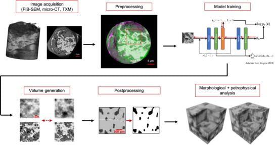
6]. Latent space is a learned representation of the data space that has a known and tractable distribution that enables sampling images. Our approach allows for more stable training on larger image slices than previously proposed models; parallel generation of image slices in an image volume; and a first model that generalizes 3D volume synthesis to grayscale, two-dimensional, and multimodal datasets. In what follows, we present an overview of generative modeling for synthesis of porous media images, describe our volume generation method, and apply our method to several 2D and 3D image datasets of porous media.
2. Background
2.1. Image-Based Characterization of Porous Media
High-contrast, high-resolution, and multiscale imaging technologies have become indispensable tools for the study of shale source rock [
7,
8,
9]. Many recent studies on 4D characterization and flow transport tests have used imaging techniques as the foundation of their investigations, including work on pore network connectivity and storage [
8,
9,
10], diffusion [
11,
12], permeability and absorption [
13], and organic matter maturation [
14,
15]. In such a workflow, images of the source rock are first acquired using techniques such as micro-CT, nuclear magnetic resonance (NMR) [
16], transmission electron microscopy [
17], or scanning electron microscopy (SEM). The images are then segmented into regions of interest, usually pore and grain phases. Then, properties such as Minkowski functionals [
18,
19], permeability, or mercury intrusion capillary pressure are computed. When the imaging modality is nondestructive, as with micro-CT or NMR, this approach allows for characterization of a sample while preserving the sample for further experimentation.
Image-based characterization, while powerful, is often challenging due to the limited availability of high-resolution/high-contrast imaging data. Nanoscale characterization is crucial for characterization of shales but is particularly difficult due to factors such as limited availability of imaging machines, potentially large costs, and the time and expertise required to prepare samples and to acquire image data. Recent interest in deep learning-based methods for source rock characterization has only grown the need for large amounts of imaging data. A sizable body of work therefore has focused on developing generative models to create synthetic data to improve characterization, and in recent years, the focus has shifted to applying deep learning generative models to source rock images.
2.2. Deep Generative Models Overview
Generative models seek to learn the probability distribution of data or to create new data samples. These are in contrast to discriminative models that predict a response value from input data. Deep generative models are deep learning-based models that either model the probability distribution of training data using a deep neural network or train a neural network to sample datapoints from the training data distribution. The most popular deep generative models include generative adversarial networks (GANs) [
20], variational autoencoders (VAEs) [
21], and autoregressive models [
22].
GANs consist of two networks: a generator and discriminator. During training, these two networks play a minimax game against each other: the generator network attempts to synthesize realistic datapoints and the discriminator classifies an input sample as real or fake. At convergence, this approach generates datapoints that are statistically indistinguishable from the training data. By feeding latent random noise vectors into the generator network, we are then able to sample new datapoints.
VAEs train an encoder network to project data into a latent space with a known distribution and a decoder network to transform latent space vectors back into data space. This allows for sampling new datapoints by passing latent space vectors of known distribution into the decoder network. Both GANs and VAEs allow for a latent representation of datapoints but cannot provide the likelihood for a given datapoint.
Autoregressive models seek to model the probability distribution of the data by predicting the next datapoint in a series using previous datapoints. These models are trained to predict successive datapoints from past datapoints by maximizing the likelihood of a given sequence. Autoregressive models have the advantage of providing an exact likelihood computation for a given sequence of data but do not provide a latent representation of data and can be impractical for modeling images because they are inherently not parallelizable [
22].
2.3. Synthesis of Geologic Samples
Generative modeling for porous media samples has primarily revolved around two families of techniques: statistical and deep learning methods. Statistical methods treat the phase of a given pixel or voxel as a Bernoulli random variable for which the value is determined by an underlying random process. These techniques tend to fall into either multi-point statistics (MPS) [
23] or simulated annealing-based methods [
24]. MPS methods have been shown to generate effectively microscale images even from relatively sparse training data [
1,
25,
26], but they may be very slow. Furthermore, MPS methods may have difficulty capturing long-range and multiscale features [
27,
28,
29]. This difficulty significantly impacts reconstruction of shale volumes due to the multiscale nature of shales [
30]. Simulated-annealing methods incorporate multiple correlation functions and capture larger-scale features, but they can take hours or even days to generate large volumes [
31,
32].
More recent work has focused on using deep generative models to synthesize porous media images. While this work has been more limited than statistical methods, these methods represent an emerging and powerful class of techniques for porous media synthesis. Mosser et al. [
3] applied deep convolutional GANs (DCGANs), a variant of GANs where the generator and discriminator network are convolutional neural networks (CNNs), to generate sandstone and limestone images from binarized micro-CT data. The results from this work showed close agreement with ground-truth values for topological and flow features of the rock samples, and further work was able to generalize this model to generate arbitrarily large image volumes [
33]. The major drawback of a DCGAN-based approach is that DCGANs require 3D training data to synthesize 3D image volumes. This limits the number of applications, especially in shale fabric reconstruction. Other related work on shale image reconstruction has focused on reconstructing fine-scale features from coarse-scale images of shales [
34] or on assimilating multimodal imaging data [
35]. However, beyond these studies, there is little work on synthesizing or reconstructing source rock images using deep generative models.
A persistent challenge in generating porous media is synthesizing 3D image volumes when only 2D training data is available [
36]. So far, only statistical methods have been able to address this problem. These approaches model the source rock as a two-phase isotropic porous medium and optimize the 3D data such that the 2D correlation function matches that of the training data [
37]. These methods may be highly efficient and able to synthesize entire image volumes from a single 2D training image [
27]. However, given the importance of grayscale features and multimodal images for shale fabric characterization, there exists a need for an approach that is able to synthesize 3D volumes from 2D image data. Generalization to any type of porous medium images, including grayscale and multimodal, is also needed.
3. Methodology
In this work, we introduce RockFlow, a porous media volume synthesis algorithm using generative flow models [
4,
5,
6]. To the best of our knowledge, RockFlow is the first attempt to apply generative flow models to the synthesis of porous media images. Below, we give an overview of generative flow models, the porous media volume synthesis algorithm introduced here, and steps for calculating the latent space representations used to generate the porous media volumes.
3.1. Generative Flow Models
Generative flow models were originally introduced in [
4] and further generalized in [
5,
6,
38]. At a high level, these models train a bijective mapping between data space and a latent space of known distribution. Because the mapping is bijective, we exactly computed the likelihood of a given datapoint using the change of variables formula. In doing so, generative flow models combine the latent representation property of GANs and VAEs with the exact likelihood property of autoregressive models.
Generative flow models are trained to maximize the likelihood of the observed datapoints in the dataset
. This is equivalent to minimizing the negative log-likelihood of the datapoints
:
From here, we chose our latent vectors
to follow a given distribution
and model our datapoints
, where
is an invertible function or composition of invertible functions. Let
. Then, we computed the log-likelihood of the sampled data point as follows:
using the change of variable formula for probability distributions and defining
,
, and
. By using this change of variables, we recasted the likelihood computation for the datapoint
in terms of the tractable likelihood for the latent representation
. Assuming the functions
are sufficiently smooth, the generator function
allows for interpolation between latent vectors
.
In this work, we used the
Glow model from Kingma and Dhariwal [
6]. The model is summarized in
Figure 1. Each of the
L steps of the flow contains a squeeze step; a flow step consisting of an actnorm layer,
invertible convolution, and an affine coupling layer; and a split layer. At sampling time, we fed noise of a known distribution into the reversed network to produce a synthetic data sample. We refer the reader to [
6] for further details on the model and its implementation. Is the italic format of word “Glow” in the sentence before “The model” necessary? If yes, please unifrom it all the text.
3.2. Volume Generation Approach
The latent space interpolation property is the most important feature of generative flow models that the RockFlow algorithm exploits. This property states that a linear combination of latent representation vectors in latent space produces a semantic interpolation in image space. The property is illustrated in
Figure 2. Latent space interpolation is widely observed in generative flow models as well as other deep generative models such as GANs.
Our method exploits the latent space interpolation property in conjunction with the isotropic nature of porous media samples to generate 3D volumes by training only on 2D input data. The volume generation algorithm is given in Algorithm 1. In this workflow, we first trained a generative flow model on 2D image slices. To generate the volume, we selected “anchor slices” with fixed latent space vectors, interpolated between the anchor slices by taking an affine combination between the latent representations of the nearest anchor slices, and calculated the image slices corresponding to each of the computed latent representations.
| Algorithm 1 RockFlow algorithm with glow models. |
![Energies 13 06571 i001]() |
The volume generation process is depicted in
Figure 3. In this example, only two interpolation steps are taken between anchor slices. In practice, this quantity must be computed or set by the user. After generating volumes, the results are postprocessed to improve image quality or to correct any artifacts from model training. In particular, we found that median filtering helps reduce artifacts and that thresholding is necessary to produce binary images for morphology or permeability calculations.
Training on only 2D input data carries several advantages. First, this model is able to generalize to datasets where only 2D data is available. For inherently 2D imaging modalities such as electron microscopy, this capability allows for analysis of image volumes without relying on destructive imaging processes such as focused ion beam scanning electron microcscopy (FIB-SEM). Furthermore, our model is able to generate 3D volumes from 2D data for grayscale datasets. This is a generalization from the MPS and simulated annealing methods that only have this capability for binary images.
In addition to only requiring 2D training data, RockFlow is able to generate image slices in parallel. Computation of the latent space vectors is inexpensive and easily vectorized. Evaluation of an image volume therefore becomes equivalent to evaluating a batch of slices. This is in contrast with existing GAN-based models that must train on and generate entire image volumes simultaneously.
3.3. Latent Vector Calculation
The accuracy of the RockFlow algorithm depends heavily on choosing the correct number of interpolation steps between anchor slices. In our implementation, we used the pore chord length as the number of interpolation steps. When interpolating between anchor slices, the phase of a given pixel should not change if the phase is the same in the two nearest anchor slices. The pore chord length is the average number of voxels that a pore spans. Hence, it is a natural choice for the number of interpolation steps.
To calculate the pore chord length, we first calculated the two-point covariance function:
where
is the probability that point
in the volume lies in the pore phase and
is the probability that two points separated by vector
are both in the pore phase. After computing the two-point covariance of pore phase points, we calculated the slope of the two-point covariance at the origin
using linear regression [
3,
39]. The pore length is then calculated as follows [
39]:
where
is the porosity. We rounded this to the nearest integer to find the number of interpolation steps between anchor slices. In our workflow, we based our implementation of the pore chord length following the code of Mosser et al. [
3].
A different approach calculates the number of interpolation steps by finding the likelihood-maximizing number of steps between anchor slices. However, such an approach is extremely computationally expensive because it relies on computing Monte Carlo estimates of the likelihood for full image volumes over a wide range of interpolation step sizes. Here, we used the pore chord length approach because it is straightforward and efficient to calculate when the data is easily binarized. Importantly, it is justified by known statistical properties of porous media samples [
3,
39].
3.4. Evaluation Criteria
For the baseline datasets presented below, we evaluated the models quantitatively by comparing agreement of the 3D Minkowski functionals among training and computed images. Minkowski functionals are stereological estimators providing local and global morphological information that is related to single-phase flow mechanisms [
18,
19]. In 3D, there are four Minkowski functionals that describe the geometric parameters of a set
X with a smooth surface
: volume
, surface area
, integral of mean curvature
, and Euler–Poincaré characteristic
. Here, we focused on the porosity
calculated from the volume, surface area, and Euler–Poincaré characteristic:
where
is the number of voxels in the pore phase after segmentation and
is the curvature corresponding to the maximum and minimum curvature radii, with
.
We estimated these values using the MorphoLibJ library in ImageJ [
40,
41]. The volume and porosity were implemented by directly counting the number of voxels in the pore phase and the total number of voxels. The mean breadth was computed from the Crofton formula and was proportional to the integral of the mean curvature [
42,
43]. The Euler–Poincaré characteristic in 3D describes the connectivity of the volume and was calculated as the sum of the number of vertices, edges, faces, and solids using a 6-adjacency system that considers only neighbors in the three primary directions:
We refer the reader to the documentation of the MorphoLibJ library for further details on implementation of these metrics.
4. Results
4.1. Model Training and Image Postprocessing
In all results that follow, the plane is considered the plane in the image volume along which image slices are synthesized and the z axis is the interpolation axis. The and planes therefore refer to cross sections along the interpolation direction of the synthesized image volumes.
All models are implemented in PyTorch and pre-/postprocessing done with
scikit-image and ImageJ [
44]. The glow model implementation is adapted from [
45]. For all glow models, we use affine coupling layers and temperature
during training and sampling and train using the Adam optimizer [
46] for all models. The models are trained for a differing number of epochs. We found that models for grayscale images converged in ∼25 epochs while models for binary images were trained for 100 epochs. When sampling image volumes, we also postprocess the images. The learned model may not be reversible at all points in the latent space resulting in undefined points in the output image. To compensate for this effect, we chose to convert undefined values to be the median value of our pixel values, e.g., 0.5 if all
. We also postprocess with a spherical median filter with radius
to minimize artifacts in the final reconstructed image.
Additional pre- and postprocessing are used for binary image data. We discuss these further steps below.
4.2. Baseline Datasets
Mosser et al. [
3] proposed the Berea sandstone and Ketton limestone binary
-CT images as baseline datasets for rock image generation. We therefore began by evaluating our volume generation algorithm on these datasets as a point of comparison with the previously proposed DCGAN model in [
3].
During training, we discovered that the chosen generative flow model is unable to train on binary image data. When training on unprocessed binary data, the model either collapses to outputting all undefined pixels or exhibits extremely slow convergence. We believe this is because binary images are equivalent to very high contrast images, and therefore, it is too difficult for the model to map effectively between these input image and the desired latent space.
To address this issue, we preprocess our images by applying a small blur kernel and by clamping the values. Let
I be the original binary image with all pixels
. Our preprocessing step is then as follows:
This preprocessing pipeline, in effect, creates synthetic micro-CT data by restoring the edge blurring present in natural sandstone and limestone images and by moving grayscale values away from the extremes of the pixel value range. An example of this preprocessing is shown in
Figure 4. We found that this preprocessing pipeline allowed for significantly improved model convergence and stability over training on raw binary data. Indeed, when training on the binary datasets, the models without this preprocessing in their data pipelines almost never converged while the models with preprocessing almost always converged. While we did not explore the effect of the truncation values on the results, we do observe that using values that are symmetric about the median pixel value does improve results.
Example synthetic and ground-truth slices are shown in
Figure 5 and
Figure 6. In our postprocessing pipeline, we apply a
spherical median filter to eliminate artifacts such as undefined pixels or “jittering” of grain-pore boundaries between slices and segment using Otsu thresholding [
47].
We also evaluated quantitative topological metrics for the synthesized samples and compared them to the ground-truth sample and DCGAN model. These results are summarized in
Figure 7 for the Berea sample and
Figure 8 for the Ketton sample. The data for the ground-truth images and DCGAN model are taken from Mosser et al. [
3]. The ground-truth and DCGAN values were evaluated for
voxel volumes, while our results are only for
volumes. This difference in evaluation volumes reflects one shortcoming of our model: DCGAN models are fully convolutional and therefore can be evaluated for an arbitrarily large volume at sample time [
33], but the RockFlow model has fixed dimensions in the training image plane i.e., the
plane. From the quantitative results, we see that the RockFlow model underestimates porosity for the Berea sandstone model, overestimates surface area for both samples, and obtains a close match for the Euler characteristic for both baseline training samples.
4.3. Volume Generation from 2D Data
The biggest advantage of RockFlow over existing porous media synthesis algorithms is the ability to synthesize 3D grayscale image volumes from 2D training data. Many important imaging modalities for shale characterization, such as electron microscopy, only acquire 2D image data. While some techniques, such as FIB-SEM, reconstruct image volumes with the resolution and contrast of SEM images by successively milling and imaging a sample, this is at the expense of destroying the sample during image acquisition. Grayscale values in shale electron microscopy images carry important information about pore space, kerogen content, and mineral composition. Consequently, binary image volume generation methods cannot reconstruct all desired features of shale images. The RockFlow algorithm is able to generate grayscale images in 3D from data acquired only in 2D.
To demonstrate this capability, we train a model to synthesize image volumes for a shale FIB-SEM dataset. The FIB-SEM dataset was acquired for a
m Bakken shale sample and comprises 787 slices approximately 5 nm apart with a voxel size of
nm [
48,
49]. We downsampled these images to have resolution
nm so that the field of view of the training image patches is increased.
Figure 9 shows a full training image and synthesized image slices, and
Figure 10 shows a rendering of a reconstructed volume with orthoslice cutouts. The interpolation step size was chosen manually for generation of these image volumes because shale images are not easily segmented using Otsu thresholding. Qualitatively, the synthetic images resemble the training images in both the training plane (
images) and synthesized plane (
images). The rendered volume shows that our method is capable of synthesizing realistic grayscale FIB-SEM data for shale samples.
4.4. Multimodal Image Synthesis
A key emerging method for shale characterization is multimodal imaging to infer unknown image data by assimilating data from multiple modalities, such as predicting high-contrast destructive imaging data from low-contrast nondestructive data or enhancing low-resolution images using single image super-resolution methods. Such image translation and super-resolution models require large amounts of imaging data to train. However, multimodal data can be challenging, time-intensive, or sample-destructive to acquire and, therefore, are not always practical in experimental setups. The capability to synthesize grayscale multimodal image data of porous media samples from 2D data allows for training paired image translation and super-resolution models [
50] for multimodal/multiscale data using synthetic data without needing to directly acquire 3D multimodal data.
Towards these applications, we present results for synthesizing multimodal imaging data from 2D training data. The dataset used is 2D aligned transmission X-ray microscopy (TXM) and FIB-SEM nanoscale images acquired for a Vaca Muerta shale sample. Such a dataset is usable for training image translation models to predict high-contrast, sample-destructive FIB-SEM data from low-contrast nondestructive TXM data [
35]. We synthesized the multimodal data by training the multimodal image as a 2-channel input image to the flow model.
Figure 11 shows example training images and generated
px image patches for dual modality TXM and FIB-SEM data. The synthetic images closely resemble the training data and are applicable to image translation models. We also render an image volume, shown in
Figure 12. The rendered image does contain some artifacts in the TXM volume along the
z-axis. However, the rendered volume nevertheless demonstrates the ability of the RockFlow model to synthesize jointly multimodal 3D data from 2D training data. This opens up many applications to other image modalities where 3D information is desired but only 2D information is available.
5. Discussion
The results from the grayscale image volume generation show that the RockFlow model reconstructs realistic porous media images from 2D training data. Both the FIB-SEM and dual modality TXM/FIB-SEM synthetic images closely resemble the training data. Thus, these models may be applied to quantify properties of the shale fabric from image data or to generate synthetic training data for other image processing tasks such as image translation.
The results from the binary data highlight some of the difficulties of our model. First, we found that training models to convergence on raw binary data is nearly impossible, even when the pixel values are clamped away from the extreme values. It was only by applying a mean blur filter that the model was able to learn the binary data. This limitation presents a significant challenge when grayscale data is not available. However, when acquiring and analyzing data for new samples, this limitation should not be a factor, as all CT image data begins as grayscale before binarizing.
The results for evaluating morphological properties of the baseline samples are mixed. For both samples, the RockFlow model overestimates the surface area and correctly matches the Euler characteristic. We believe that the surface area is overestimated due to artifacts present in images generated with this method. The results in [
51] show that RockFlow applied to a grayscale Bentheimer sandstone dataset is able to match closely the spatial covariance, Minkowski functionals, and permeability of the ground-truth sample. Accordingly, we conclude that the baseline results are not due to an inherent limitation of our algorithm but rather due to difficulty pre-/postprocessing binary data for flow models.
The training dynamics for both the grayscale and binary image models further demonstrate that the presented method is more readily applied to grayscale datasets than binary data.
Figure 13 shows the training dynamics for the Berea sandstone model with binary images and the FIB-SEM model. We see that the FIB-SEM model converges much more quickly, obtaining good images in <10 epochs and fully converging within 25 epochs. The Berea sandstone model meanwhile still has sampling errors after 100 epochs of training, further demonstrating the difficulty of training RockFlow models on binary data.
Reconstruction for binary datasets can be improved by modifying the postprocessing pipeline. For the results presented here, we only apply an spherical median filter to remove some of the artifacts associated with the interpolation. However, more advanced postprocessing strategies for inpainting undefined pixels or for removing other artifacts could be developed. The artificial blurring of the binary images may also be the cause of reduced porosity and surface area, so a postprocessing method compensating for closure of the pores could improve the porosity and surface area results.
Indeed, postprocessing can greatly affect the qualitative performance of the presented model.
Figure 14 shows
plane slices for synthesized Berea sandstone images with different radii for a spherical median filter applied after image generation. The median filter is able to mitigate some of the “jittering” effect between slices. However, as shown by the
images, a larger median filter kernel can distort the image significantly and can remove small features present in the image.
6. Summary
RockFlow is a fundamentally new method for synthesizing porous media samples that only requires 2D training images, is generalized to grayscale and multimodal images, and evaluates full image stacks in parallel. To the best of our knowledge, this is the first porous media synthesis algorithm that generates 3D grayscale data from 2D images. We apply our model to baseline datasets and show that the model closely matches the Euler characteristic; overestimates surface area; and for one baseline sample, underestimates porosity. We also demonstrate the ability of our model to generate realistic nano-scale FIB-SEM volumes and multimodal image data, an important emerging method for shale fabric characterization.
Future work on the RockFlow model will focus on two main avenues. First, the binary data handling pipeline should be improved. While we were able to train the models stably and to generate sample images, the performance for our model lags behind that of the DCGAN model from [
3] for the baseline binary datasets. We believe that, with improved pre- and postprocessing of binary image data, it is possible to obtain performance comparable to GAN-based models for the baseline datasets. Possible directions could include an improved pipeline for input data to the network and a check on the thresholding value used during postprocessing to match known or expected porosity of the sample.
The second area of future work focuses on application of this model to other imaging datasets. Guan et al. [
51] have applied this model to a Bentheimer sandstone, but there remains much room for further applications, specifically for shale image synthesis and characterization. Multimodal image synthesis for shale fabric characterization and multiscale image synthesis—e.g., joint generation of CT and micro-CT images—are promising areas. We believe that RockFlow is particularly applicable to nanoscale multimodal characterization of shales due to our algorithm’s ability to generate 3D samples even from 2D electron microscopy data.
While the performance for the baseline binary datasets can be improved, the presented algorithm has many applications for porous media characterization and specifically for analysis and characterization of shale fabrics. This algorithm is capable of generating 3D grayscale rock volumes from 2D data, which will greatly expand our ability to characterize petrophysical properties of source rock samples using nondestructive, multimodal, or limited image data. With further development, RockFlow will become a useful tool for image-based characterization of porous media.
Author Contributions
T.I.A. developed and implemented the presented image volume synthesis algorithm. K.M.G. developed the image evaluation pipeline and assisted with development of the image synthesis algorithm by testing the algorithm multiple datasets. B.V. acquired and curated the multimodal TXM/SEM datasets. S.A.A. advised on portions of this project related to shales. A.R.K. was the principal investigator, acquired funding, and supervised the work for this project. All authors have read and agreed to the published version of the manuscript.
Funding
This work was supported as part of the Center for Mechanistic Control of Water-Hydrocarbon-Rock Interactions in Unconventional and Tight Oil Formations (CMC-UF), an Energy Frontier Research Center funded by the U.S. Department of Energy (DOE), Office of Science, Basic Energy Sciences (BES), under award # DE-SC0019165. T.A. acknowledges the Siebel Scholars Foundation.
Acknowledgments
The authors thank Mohammad Piri and Soheil Saraji for kindly sharing the FIB-SEM data. The authors also thank Cynthia M. Ross, Laura Frouté, Manju Murugesu, and Yulman Perez-Claro for many helpful discussions.
Conflicts of Interest
The authors declare no conflict of interest.
References
- Okabe, H.; Blunt, M.J. Prediction of permeability for porous media reconstructed using multiple-point statistics. Phys. Rev. E Stat. Phys. Plasmas Fluids Relat. Interdiscip. Top. 2004, 70, 066135. [Google Scholar] [CrossRef] [PubMed] [Green Version]
- Okabe, H.; Blunt, M.J. Pore space reconstruction using multiple-point statistics. J. Pet. Sci. Eng. 2005, 46, 121–137. [Google Scholar] [CrossRef]
- Mosser, L.; Dubrule, O.; Blunt, M.J. Reconstruction of three-dimensional porous media using generative adversarial neural networks. Phys. Rev. E 2017, 96. [Google Scholar] [CrossRef] [PubMed] [Green Version]
- Dinh, L.; Krueger, D.; Bengio, Y. NICE: Non-linear independent components estimation. In Proceedings of the 3rd International Conference on Learning Representations, ICLR 2015—Workshop Track Proceedings, San Diego, CA, USA, 7–9 May 2015; Volume 1, pp. 1–13. [Google Scholar]
- Dinh, L.; Sohl-Dickstein, J.; Bengio, S. Density estimation using real NVP. In Proceedings of the 5th International Conference on Learning Representations, ICLR 2017—Conference Track Proceedings, Toulon, France, 24–26 April 2017. [Google Scholar]
- Kingma, D.P.; Dhariwal, P. Glow: Generative flow with invertible 1 × 1 convolutions. In Proceedings of the Advances in Neural Information Processing Systems, Montreal, QC, Canada, 3–8 December 2018; pp. 10215–10224. [Google Scholar]
- Vega, B.; Andrews, J.C.; Liu, Y.; Gelb, J.; Kovscek, A. Nanoscale visualization of gas shale pore and textural features. In Proceedings of the Unconventional Resources Technology Conference, Denver, CO, USA, 12–14 August 2013; pp. 1603–1613. [Google Scholar]
- Ketcham, R.A.; Carlson, W.D. Acquisition, optimization and interpretation of x-ray computed tomographic imagery: Applications to the geosciences. Comput. Geosci. 2001, 27, 381–400. [Google Scholar] [CrossRef]
- Blunt, M.J. Multiphase Flow in Permeable Media: A Pore-Scale Perspective; Cambridge University Press: Cambridge, UK, 2017. [Google Scholar] [CrossRef]
- Aljamaan, H.; Ross, C.M.; Kovscek, A.R. Multiscale Imaging of Gas Storage in Shales. SPE J. 2017, 22, 1–760. [Google Scholar] [CrossRef]
- Alnoaimi, K.R.; Duchateau, C.; Kovscek, A. Characterization and measurement of multi-scale gas transport in shale core samples. In Proceedings of the Unconventional Resources Technology Conference, Denver, CO, USA, 25–27 August 2014; pp. 1140–1158. [Google Scholar]
- Zhang, Y.; Mostaghimi, P.; Armstrong, R.T.; Fogden, A.; Arena, A.; Sheppard, A.; Middleton, J. Determination of Local Diffusion Coefficients and Directional Anisotropy in Shale From Dynamic Micro-CT Imaging. In Proceedings of the Unconventional Resources Technology Conference, Austin, TX, USA, 24–26 July 2017; pp. 3083–3095. [Google Scholar]
- Aljamaan, H.; Alnoaimi, K.; Kovscek, A. In-depth experimental investigation of shale physical and transport properties. In Proceedings of the Unconventional Resources Technology Conference, Denver, CO, USA, 12–14 August 2013; pp. 1120–1129. [Google Scholar]
- Panahi, H.; Kobchenko, M.; Renard, F.; Mazzini, A.; Scheibert, J.; Dysthe, D.K.; Jamtveit, B.; Malthe-Sørenssen, A.; Meakin, P. A 4D synchrotron X-ray tomography study of the formation of hydrocarbon migration pathways in heated organic-rich shale. arXiv 2014, arXiv:1401.2448. [Google Scholar] [CrossRef]
- Kim, T.W.; Ross, C.M.; Guan, K.M.; Burnham, A.K.; Kovscek, A.R. Permeability and Porosity Evolution of Organic-Rich Shales from the Green River Formation as a Result of Maturation. SPE J. 2020. [Google Scholar] [CrossRef]
- Washburn, K.E.; Birdwell, J.E. Updated methodology for nuclear magnetic resonance characterization of shales. J. Magn. Reson. 2013, 233, 17–28. [Google Scholar] [CrossRef]
- Froute, L.; Kovscek, A.R. Nano-Imaging of Shale using Electron Microscopy Techniques. In Proceedings of the Unconventional Resources Technology Conference (URTEC), 20–22 July 2020. [Google Scholar]
- Mecke, K.; Arns, C.H. Fluids in porous media: A morphometric approach. J. Phys. Condens. Matter 2005, 17. [Google Scholar] [CrossRef]
- Arns, C.H.; Knackstedt, M.A.; Mecke, K. 3D structural analysis: Sensitivity of Minkowski functionals. J. Microsc. 2010, 240, 181–196. [Google Scholar] [CrossRef]
- Goodfellow, I.J.; Pouget-abadie, J.; Mirza, M.; Xu, B.; Warde-farley, D. Generative-Adversarial-Nets. Nips 2014, 1–9. [Google Scholar] [CrossRef]
- Kingma, D.P.; Welling, M. Auto-Encoding Variational Bayes. arXiv 2013, arXiv:1312.6114. [Google Scholar]
- Van den Oord, A.; Kalchbrenner, N.; Kavukcuoglu, K. Pixel Recurrent Neural Networks. arXiv 2016, arXiv:1601.06759. [Google Scholar]
- Caers, J. Geostatistical reservoir modelling using statistical pattern recognition. J. Pet. Sci. Eng. 2001, 29, 177–188. [Google Scholar] [CrossRef]
- Manwart, C.; Torquato, S.; Hilfer, R. Stochastic reconstruction of sandstones. Phys. Rev. E Stat. Phys. Plasmas Fluids Relat. Interdiscip. Top. 2000, 62, 893–899. [Google Scholar] [CrossRef] [Green Version]
- Okabe, H.; Blunt, M.J. Pore space reconstruction of vuggy carbonates using microtomography and multiple-point statistics. Water Resour. Res. 2007, 43, 3–7. [Google Scholar] [CrossRef]
- Bai, T.; Tahmasebi, P. Hybrid geological modeling: Combining machine learning and multiple-point statistics. Comput. Geosci. 2020, 142, 104519. [Google Scholar] [CrossRef]
- Tahmasebi, P.; Hezarkhani, A.; Sahimi, M. Multiple-point geostatistical modeling based on the cross-correlation functions. Comput. Geosci. 2012, 16, 779–797. [Google Scholar] [CrossRef]
- Tahmasebi, P.; Sahimi, M.; Caers, J. MS-CCSIM: Accelerating pattern-based geostatistical simulation of categorical variables using a multi-scale search in Fourier space. Comput. Geosci. 2014, 67, 75–88. [Google Scholar] [CrossRef]
- Tahmasebi, P.; Sahimi, M.; Andrade, J.E. Image-based modeling of granular porous media. Geophys. Res. Lett. 2017, 44, 4738–4746. [Google Scholar] [CrossRef] [Green Version]
- Mehmani, Y.; Anderson, T.; Wang, Y.; Aryana, S.A.; Battiato, I.; Tchelepi, H.A.; Kovscek, A. Striving to Translate Shale Physics across Ten Orders of Magnitude: What Have We Learned? Earth Sci. Rev. 2020, submitted. [Google Scholar]
- Čapek, P.; Hejtmánek, V.; Brabec, L.; Zikánová, A.; Kočiřík, M. Stochastic reconstruction of particulate media using simulated annealing: Improving pore connectivity. Transp. Porous Media 2009, 76, 179–198. [Google Scholar] [CrossRef]
- Pant, L.M.; Berkeley, L. Stochastic Characterization and Reconstruction of Porous Media. Ph.D. Thesis, University of Alberta, Edmonton, AB, Canada, 2016. [Google Scholar] [CrossRef]
- Mosser, L.; Dubrule, O.; Blunt, M.J. Conditioning of three-dimensional generative adversarial networks for pore and reservoir-scale models. arXiv 2018, arXiv:1802.05622, 1–5. [Google Scholar]
- Kamrava, S.; Tahmasebi, P.; Sahimi, M. Enhancing images of shale formations by a hybrid stochastic and deep learning algorithm. Neural Netw. 2019, 118, 310–320. [Google Scholar] [CrossRef]
- Anderson, T.I.; Vega, B.; Kovscek, A.R. Multimodal imaging and machine learning to enhance microscope images of shale. Comput. Geosci. 2020, 145, 104593. [Google Scholar] [CrossRef]
- Adler, P.; Jacquin, C.; Quiblier, J. Flow in simulated porous media. Int. J. Multiph. Flow 1990, 16, 691–712. [Google Scholar] [CrossRef]
- Roberts, A.P. Statistical reconstruction of three-dimensional porous media from two-dimensional images. Phys. Rev. E 1997, 56, 3203–3212. [Google Scholar] [CrossRef] [Green Version]
- Papamakarios, G.; Nalisnick, E.; Rezende, D.J.; Mohamed, S.; Lakshminarayanan, B. Normalizing Flows for Probabilistic Modeling and Inference. arXiv 2019, arXiv:1912.02762. [Google Scholar]
- Torquato, S. Random Heterogeneous Materials: Microstructure and Macroscopic Properties. In Interdisciplinary Applied Mathematics; Springer: New York, NY, USA, 2005. [Google Scholar]
- Legland, D.; Arganda-Carreras, I.; Andrey, P. MorphoLibJ: Integrated library and plugins for mathematical morphology with ImageJ. Bioinformatics 2016, 32, 3532–3534. [Google Scholar] [CrossRef] [Green Version]
- Doube, M.; Kłosowski, M.M.; Arganda-Carreras, I.; Cordelières, F.P.; Dougherty, R.P.; Jackson, J.S.; Schmid, B.; Hutchinson, J.R.; Shefelbine, S.J. BoneJ: Free and extensible bone image analysis in ImageJ. Bone 2010, 47, 1076–1079. [Google Scholar] [CrossRef] [Green Version]
- Serra, J.P.; Serra, J.; Cressie, N.A.C. Number v. 1 Image Analysis and Mathematical Morphology. In Image Analysis and Mathematical Morphology; Academic Press: Cambridge, MA, USA, 1982. [Google Scholar]
- Ohser, J.; Schladitz, K. 3D Images of Materials Structures: Processing and Analysis; Wiley: Hoboken, NJ, USA, 2009. [Google Scholar]
- Schindelin, J.; Arganda-Carreras, I.; Frise, E.; Kaynig, V.; Longair, M.; Pietzsch, T.; Preibisch, S.; Rueden, C.; Saalfeld, S.; Schmid, B.; et al. Fiji: An open-source platform for biological-image analysis. Nat. Methods 2012, 9, 676–682. [Google Scholar] [CrossRef] [PubMed] [Green Version]
- Van Amersfoort, J. Glow-PyTorch. 2019. Available online: https://github.com/y0ast/Glow-PyTorch (accessed on 2 November 2020).
- Kingma, D.P.; Ba, J. Adam: A Method for Stochastic Optimization. arXiv 2014, arXiv:1412.6980. [Google Scholar]
- Otsu, N. A Threshold Selection Method from Gray-Level Histograms. IEEE Trans. Syst. Man Cybern. 1979, 9, 62–66. [Google Scholar] [CrossRef] [Green Version]
- Aryana, S.; Ross, C.; Saraji, S. Development of a nanofluidic chip representative of a shale sample. In Proceedings of the AGU Fall Meeting, San Francisco, CA, USA, 14–18 December 2015. H21N-06. [Google Scholar]
- Saraji, S.; Piri, M. The representative sample size in shale oil rocks and nano-scale characterization of transport properties. Int. J. Coal Geol. 2015, 146, 42–54. [Google Scholar] [CrossRef]
- Isola, P.; Zhu, J.Y.; Zhou, T.; Efros, A.A. Image-to-image translation with conditional adversarial networks. In Proceedings of the 30th IEEE Conference on Computer Vision and Pattern Recognition, CVPR 2017, Honolulu, HI, USA, 21–26 July 2016; pp. 5967–5976. [Google Scholar] [CrossRef] [Green Version]
- Guan, K.; Anderson, T.; Cruex, P.; Kovscek, A. Reconstructing Porous Media Using Generative Flow Networks. Comput. Geosci. 2020. in review. [Google Scholar]
Figure 1.
Glow model architecture adapted from [
6]: during training (black arrows), the image is passed into the network, and successive flow steps transform the data into a vector
that follows a Gaussian distribution. During sampling (red arrows), vectors
are sampled from
and fed into the reversed network.
Figure 2.
Depiction of the linear interpolation property of the RockFlow porous media generation algorithm (top). For generative flow models, linear interpolation in the latent space is equivalent to semantic interpolation in image space (bottom).
Figure 2.
Depiction of the linear interpolation property of the RockFlow porous media generation algorithm (top). For generative flow models, linear interpolation in the latent space is equivalent to semantic interpolation in image space (bottom).
Figure 3.
Image volume generation algorithm: (a) anchor slices are sampled by choosing random vectors zi according to the prior optimized during model training and then by sampling the corresponding rock image slices. For automatic step number computation, these images are binarized and the pore chord length is computed. (b) Linear combinations of the anchor slice latent vectors are computed, and the intermediate image slices are evaluated to create the full image volume. Evaluation of all volume slices can be done in parallel. (c) Postprocessing was performed for generated images. Applying a spherical median filter to the generated images improves the resulting output images. Images are optionally segmented using Otsu thresholding to create a final image binary for quantifying spatial statistics or for performing flow simulations. Other segmentation algorithms or software could be used, but we leave this as an area for future exploration.
Figure 4.
Illustration of preprocessing for input images: without preprocessing the binarized input images, the glow models do not converge during training. (a) Original binary image patch; (b)grayscale preprocessed image patch.
Figure 4.
Illustration of preprocessing for input images: without preprocessing the binarized input images, the glow models do not converge during training. (a) Original binary image patch; (b)grayscale preprocessed image patch.
Figure 5.
Berea example images with resolution at 3.0 μm/voxel: (a–d) ground-truth training images in the x − y plane, (e–h) binarized synthetic images taken from the x − y plane, and (i–l) binarized synthetic images taken from the x − z plane.
Figure 5.
Berea example images with resolution at 3.0 μm/voxel: (a–d) ground-truth training images in the x − y plane, (e–h) binarized synthetic images taken from the x − y plane, and (i–l) binarized synthetic images taken from the x − z plane.
Figure 6.
Ketton example images with resolution at 15.2 μm/voxel: (a–d) ground-truth training images in the x − y plane, (e–h) binarized synthetic images taken from the x − y plane, and (i–l) binarized synthetic images taken from the x − z plane.
Figure 6.
Ketton example images with resolution at 15.2 μm/voxel: (a–d) ground-truth training images in the x − y plane, (e–h) binarized synthetic images taken from the x − y plane, and (i–l) binarized synthetic images taken from the x − z plane.
Figure 7.
Comparison of Minkowski functionals among ground-truth images, DCGAN model, and the presented generative flow model for Berea sandstone images for (left) porosity, (middle) surface area, and (right) Euler characteristic. The ground-truth and DCGAN data were evaluated on
image volumes and taken from [
3]. The generative flow model was evaluated on
image volumes.
Figure 8.
Comparison of Minkowski functionals among ground-truth images, DCGAN model, and the presented generative flow model for Ketton sample images for (left) porosity, (middle) surface area, and (right) Euler characteristic. The ground-truth and DCGAN data were evaluated on
image volumes and taken from [
3]. The generative flow model was evaluated on
image volumes.
Figure 9.
(a) Example training image for FIB-SEM image, (b–e) x − y plane images for synthesized image volume, and (f–i) x − z plane images for synthesized image volume: the sampled images are 128 × 128 px patches. All images have 9.39 × 8.97 nm/voxel resolution in the x − y plane.
Figure 9.
(a) Example training image for FIB-SEM image, (b–e) x − y plane images for synthesized image volume, and (f–i) x − z plane images for synthesized image volume: the sampled images are 128 × 128 px patches. All images have 9.39 × 8.97 nm/voxel resolution in the x − y plane.
Figure 10.
Volume rendering of synthetic FIB-SEM images with orthoslice cutouts shown. The images are trained on pixel image patches and a image volume is synthesized.
Figure 10.
Volume rendering of synthetic FIB-SEM images with orthoslice cutouts shown. The images are trained on pixel image patches and a image volume is synthesized.
Figure 11.
Training slices and synthesized multimodal slices with resolution of 62.4 μm/voxel: (c–f) synthetic TXMimage patches and (g–j) synthetic SEM image patches corresponding to the generated TXM images.
Figure 11.
Training slices and synthesized multimodal slices with resolution of 62.4 μm/voxel: (c–f) synthetic TXMimage patches and (g–j) synthetic SEM image patches corresponding to the generated TXM images.
Figure 12.
Dual-modality (a) TXM and (b) SEM 3D image volumes generated for a Vaca Muerta shale sample.
Figure 12.
Dual-modality (a) TXM and (b) SEM 3D image volumes generated for a Vaca Muerta shale sample.
Figure 13.
Learning curves for (a) Berea sandstone model and (b) FIB-SEM image datasets that are binary and grayscale images, respectively. We see that training is much slower for the binary images, and there are still more sampling errors after 50 epochs of training than 25 epochs for the grayscale images.
Figure 14.
Comparison of different amounts of median filtering applied to the same synthesized image volume for the Berea sandstone model: images are taken from the x − z plane of a generated image volume. As the size of the spherical median filter is increased, there is less jittering between image slices and undefined pixels are eliminated, but smaller details are lost. (a) Original; (b) Binary; (c) r = 1; (d) r = 3.
| Publisher’s Note: MDPI stays neutral with regard to jurisdictional claims in published maps and institutional affiliations. |
© 2020 by the authors. Licensee MDPI, Basel, Switzerland. This article is an open access article distributed under the terms and conditions of the Creative Commons Attribution (CC BY) license (http://creativecommons.org/licenses/by/4.0/).

 ,
, 


