Abstract
In this article, a modified control structure for a single-stage three phase grid-connected photovoltaic (PV) system is presented. In the proposed system, the maximum power point tracking (MPPT) function is developed using a new adaptive model-based technique, in which the maximum power point (MPP) voltage can be precisely located based on the characteristics of the PV source. By doing so, the drift problem associated with the traditional perturb and observe (P&O) technique can be easily solved. Moreover, the inverter control is accomplished using a predictive dead-beat function, which directly estimates the required reference voltages from the commanded reference currents. Then, the reference voltages are applied to a space vector pulse width modulator (SVPWM) for switching state generation. Furthermore, the proposed inverter control avoids the conventional and known cascaded loop structure of the voltage oriented control (VOC) method by elimination of the outer PI controller, and hence the overall control strategy is simplified. The proposed system is compared with different MPPT techniques, including the conventional P&O method and other techniques intended for drift avoidance. The evaluation of the suggested control methodology depends on various radiation profiles created in MATLAB. The proposed technique succeeds at capturing the maximum available power from the PV source with no drift in comparison with other methods.
1. Introduction
Renewable energy sources are getting more attention for power generation in different fields [1]. In stand-alone applications or grid-connected ones, the renewable sources have several merits with which to compete with conventional fossil fuels generators—cleanliness, availability, environment-friendliness, etc. [2,3]. Photovoltaic (PV) power is one of the promising sources among the renewable energy structures [4]. Besides the aforementioned advantages, the PV source can produce energy silently with no emissions [5]. Hydro-power is still in first place concerning the power generation level, followed by wind and PV power [6]. Recently, the policies of many countries are directed to raising the penetration of renewable energy sources [7]. That policy may be a viable option in the coming years. However, making renewable energy sources obligatory must be delayed due to the continuous lack of conventional energy sources [8].
PV system topologies can be mainly classified into two main configurations, which are the two-stage topology and the single-stage topology [9,10]. In the two-stage topology, the maximum power point tracking (MPPT) regulation is performed in the first (DC–DC) conversion stage, where a boost converter is commonly adopted between the PV energy source and the inverter for the objective of MPPT and voltage elevation. Then, the inverter manages the active and reactive power. In contrast to the two-stage topology, the MPPT function, the active power, and the reactive power are implemented in the inverter control for the single-stage configuration [11,12]. The single-stage structure is preferred from an efficiency perspective due to the decreased number of stages; i.e., no DC–DC conversion stage is why it is called single-stage topology. From control’s perspective, the two-stage configuration outweighs the single one—specifically because of the decoupling between the MPPT operation and the inverter control (active and reactive power control) [11].
Many MPPT methods have been investigated in the literature [13,14,15]. However, the most commonly adopted techniques are the perturb and observe (P&O) method and the incremental conductance (INC) one [16,17]. Even they have a similar behavior [18]. In P&O, the control parameter (voltage, current, or duty cycle) is simply perturbed in one direction. For instance, the control parameter is increased and the behavior of the power is inspected. Hence, if the power increases, the perturbation is kept in the same direction; i.e., the perturbation is further increased. Otherwise, the control parameter’s perturbation will be decreased (reversed) [19]. With INC, the operation is mainly dependent on the power–voltage (P–V) characteristics, where the derivative of this curve is positive at left side of it, negative on the right, and zero at the maximum power point (MPP) [20]. The two methods are simple to implement and free from input parameters, except for simple factors to be tuned in cases of adaptive control [16,21]. The major drawback of these methods is the continuous oscillation at steady-state [21,22]. Actually, the oscillations can be reduced by choosing a small perturbation step. However, this comes at the cost of slow tracking speed [21]. Furthermore, the conventional methods fail to extract the maximum power during fast varying atmospheric conditions (radiation) [22]. This greatly affects the PV system’s efficiency, leading to very high voltage, current, and power oscillations, which is collectively called the drift problem [23]. The main cause of this problem is that the conventional method is not capable of differentiating whether the power variation comes from the perturbation itself or from the radiation change, as a result the operating point drifting away from the MPP [23,24].
For active and reactive power management, numerous control strategies are addressed in the literature [25,26,27]. However, voltage oriented control (VOC) is the most popular technique, in which two cascaded loops are employed for active and reactive power control [28]. The outer loop or the voltage loop provides the reference current to the inner loop. Then, incorporating the feed-forward technique, the reference voltages can be computed and applied to the inverter switches using a modulator [29]. Although the inverter control utilizing the VOC method is well established in the literature, the performance of the VOC is mainly related to a proper tuning of the PI controllers’ parameters [30]. Another common technique is the direct power control (DPC), where the cascaded loop structure of the VOC is avoided and the control is carried out by comparing the reference values of the active and reactive power with their instantaneous values, and knowing the grid-voltage position, the switching states can be generated using a hysteresis controller via look-up table; thus, no modulator is required in this methodology [31]. Despite of the simple structure of the DPC method, the variable switching behavior in addition to the high power ripples are the major disadvantages of this method [32]. Recently, model predictive control (MPC) techniques became more competitive with conventional control methods [12]. MPC can be classified into finite-set model predictive control (FS-MPC) and continuous-set model predictive control (CS-MPC) [12,33]. In FS-MPC, the discrete-time structure model of the system is developed, and using a quality function design, the optimal switching state is selected. For example, and in the case of a two-level inverter, the best switching state out of eight (the eight space vectors) is selected according to the design of the cost function [34]. A significant drawback of this control strategy is the high computational burden, especially for multilevel inverters, where the cost function should be computed for all switching states [35]. Furthermore, the resulting variable switching frequency adds to the disadvantages [36]. In the case of CS-MPC, a modulator is used to obtain the switching pulses of the inverter [37].
Various techniques are presented in the literature to enhance the behavior of the conventional P&O method—specifically, the large oscillations at steady-state and the drift problem. In [23], an additional current check condition is included as a modification to the traditional P&O algorithm. However, the system is tested only by a simple step change of the radiation. Strict limitations are applied to the P&O method in [22,38] to reinforce its performance under dynamic weather conditions. However, these limitations are expected to be violated for a wide range of atmospheric variations, especially when temperature changes. A model-based MPPT technique is combined with model predictive control in [39]. The presented methodology requires some constants to be determined every sampling period, in addition to the computation load of the MPC. A multi-power-sample-based P&O algorithm is developed in [40]. This technique detects the drift problem based on the observation that the power variation will be small in case of drift occurrence; thus, multi-power-samples will help the P&O method in drift avoidance, supposing that the radiation is linearly variant. However, the methodology suffers from slow start-up tracking speed.
In this paper, an adaptive PV model-based MPPT technique is presented. The proposed method depends on calculating the MPP voltage of the PV source considering the atmospheric conditions’ variations. Thus, to avoid the confusion of the MPPT algorithm during fast radiation conditions, a radiation estimator is utilized to estimate the radiation from the measured values of voltage and current. Knowing the radiation value, the locus of the MPP voltage can be accurately computed. Then, by employing an adaptive step-size, the MPPT operates at this point. Thus, the drift problem is eliminated by capturing the estimated point. Moreover, and for faster response of active and reactive power control, the cascaded control structure of the conventional PV inverter control is eliminated by using a predictive dead-beat function with a modulator. The MPPT gives directly the reference current to the dead-beat function, which directly calculates the required reference voltages from the applied currents. Thus, a faster response of active and reactive power regulation is secured in the inverter control. The proposed methodology is a simplified control strategy with high efficiency; the effect of the MPPT algorithm and the drift problem on the quality of the injected grid currents were extensively investigated. The superiority of the presented method is proven using simulation results and compared to other drift avoidance schemes in addition to the conventional P&O. Furthermore, the proposed method was tested with several radiation profiles.
The remainder of this article is organized as follows: Section 2 introduces the model of the PV source of power and the grid-connected inverter. The drift problem, the conventional P&O method, and the proposed adaptive model-based MPPT are examined in Section 3. Section 4 discusses the modified inverter control for active and reactive power control using dead-beat predictive control. The simulation results of the proposed method using MATLAB with other published MPPT techniques are presented and discussed in Section 5. Some key points and the suggested future direction of the research in this point are addressed in Section 6. Finally, the outcome of the current study is concluded in Section 7.
2. PV System Modeling
In this study, single-stage grid-connected PV system is studied, where the model of the PV source (DC source) and the two-level inverters (inversion stage) for grid connection are presented in this section.
2.1. PV Source Investigation and Modeling
The single-diode model is used to represent the PV source characteristics. In this model, the output characteristics or the current–voltage (I–V) relationship is expressed as [12,13]
where is the photovoltaic current, n is the ideality factor of the diode, is the saturation current of the diode, is the series resistance of the PV module, is the shunt resistance of the PV module, is the thermal voltage, is the number of cells connected in series in the PV module, is the delivered current, and is the terminal voltage. The model of the circuit that describes the PV module’s non-linearity is shown in Figure 1. Furthermore, the P–V and I–V curves of the PV module at various atmospheric situations of temperature and radiation are illustrated in Figure 2, Figure 3, Figure 4 and Figure 5, respectively.
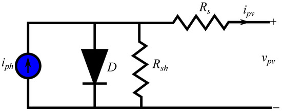
Figure 1.
Equivalent circuit of the PV module.
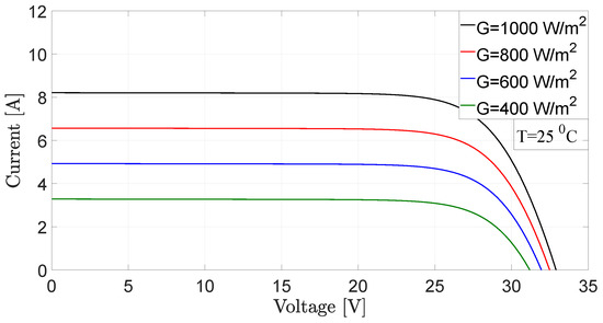
Figure 2.
I–V characteristics of the PV source for various radiation values.
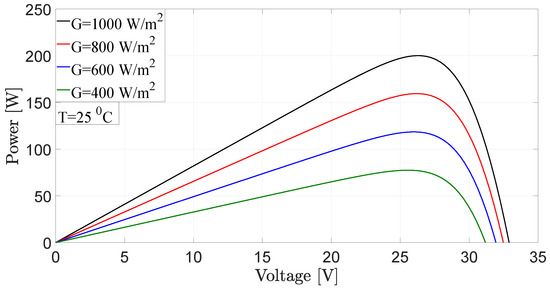
Figure 3.
P–V characteristics of the PV source for various radiation values.
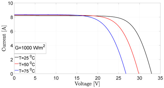
Figure 4.
I–V characteristics of the PV source for various temperature values.
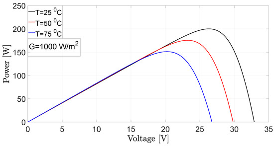
Figure 5.
P–V characteristics of the PV source for various temperature values.
It is worth mentioning that the PV module used in the simulation was KC200GT. One can observe from the P–V curve in Figure 3 that the MPP’s voltages are limited to a narrow range in the case of radiation change. In contrast, this range is wide in the case of temperature variation, as shown in Figure 5.
2.2. Two-Level Inverter Structure with the Grid
Figure 6 shows the two-level inverter tied to the grid via RL filter for power quality purposes [27]. The behavior of this system can be simply described as
where are the voltages of grid-side, are the line currents, are the inverter-side output voltages, and and are filter inductance and resistance, respectively. Further, the terminal voltages of the two-level inverter are specified by [41]
where is the DC-link voltage, represents the switching actions of the inverter, and is the transformation matrix, which can be deduced as [12,41]
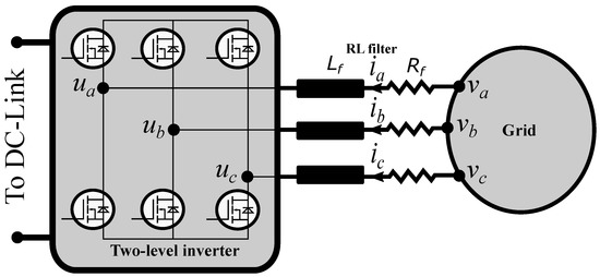
Figure 6.
Configuration of the two-level inverter with grid connection.
In the stationary reference frame (-), Equation (2) can be rewritten as
where are the line currents in reference frame. Furthermore, the representations of the voltages in the rotating (d-q) reference frame can be expressed as
where are the line currents in reference frame, and is the angular grid-frequency. Assuming that we are dealing with a balanced three phase configuration, the active and reactive power in - and d-q reference frames are obtained as
3. MPPT Techniques and Drift Problem
The goal of employing MPPT technique in PV systems is to operate as near as possible to the MPP due to the nonlinear attitude of the PV source. Unfortunately, the conventional MPPT techniques suffer from drift (divergence) of the operating point remote from the MPP. That problem happens when the system is subjected to a varying radiation profile that would be the case in cloudy days [23]. In this part of the paper, the drift problem and the proposed solution is presented.
3.1. Drift Analysis
With the help of Figure 7, it is known that at steady state, the P&O method oscillates around the MPP. Consider that the oscillation is like it is stated in Figure 7, i.e., from point 1 to 2 then 3 and vice versa. Now, suppose that the operating point is 1, so the next perturbation direction is toward point 2. At normal operation, the following operating point is 3. At this moment, assume that the radiation is increased; this makes the operating point go instantaneously to point 4 instead of 3. The MPPT algorithm notices that the power increases; thus, the perturbation is kept in the same direction, and as the radiation is increasing, the operating point will be further directed to point 5 and so on to point 6. It is clear that the operating point is drifting (diverging) from the MPP because of confusion due to the fast change of the radiation. It is worth noting that the drift here occurs to the right of the MPP. However, it can also happen to the left of the MPP based on the location of the operating point when the radiation varies [22,23].
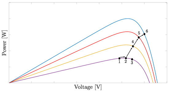
Figure 7.
Drift occurrence with the conventional P&O method for fast change of radiation.
3.2. The Traditional P&O Algorithm
The P&O method for MPPT depends on the fact that the P–V curve slope is positive on the left side, negative on the right, and zero at the top (MPP). Thus, the perturbation of the control parameter will lead to successful climbing of the hill (P–V curve), and hence the algorithm will operate closely to the peak of the curve (MPP). The conventional P&O can be implemented using different control parameters; i.e., the algorithm can be adopted for voltage, current, or even duty cycle [42], which is called direct control [43]. The major concern is the continuous oscillatory nature of P&O at steady state, which causes a significant efficiency drop. Furthermore, the conventional P&O losses the correct direction of tracking in cases of fast changing radiation conditions; thus, a very large deviation from the MPP will occur [44,45]. The algorithm of the P&O with reference current tracking is shown in Figure 8.
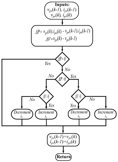
Figure 8.
Traditional P&O algorithm for MPPT.
3.3. The Proposed Adaptive Model-Based MPPT Technique
The proposed MPPT relies typically on the investigation of the PV source characteristics. Figure 9 shows the P–V characteristics of the PV source, where the MPP voltages are concentrated in a narrow range with different radiation conditions; thus, a simple approach like the constant voltage operation [46] can be employed to capture the maximum power with a moderate efficiency. Furthermore, several functions based on curve fitting tools are utilized in the literature to locate the loci of the MPP voltages. Piecewise line segments and the cubic equation were introduced in [47], while logarithmic functions are used in [48,49,50].
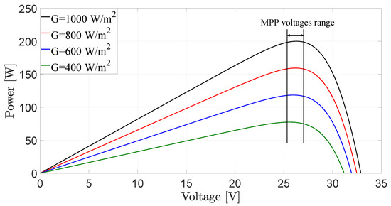
Figure 9.
MPP voltages’ variation range with different radiation conditions.
Additionally, the PV power is affected by the temperature change; thus, some MPPT techniques relate the variation of MPP voltages or currents to the temperature [51,52]. It should be mentioned that neglecting the variation of the radiation is more convenient for simple operations of MPPT, as the range of the MPP voltages is limited with radiation’s variation, but neglecting the temperature change will deteriorate the PV system’s performance, leading to extensive power reduction. The variation of the MPP voltages with temperature is linear [51], and hence neglecting the temperature effect leads the system to operate nearly at the open circuit point, as illustrated in Figure 10.
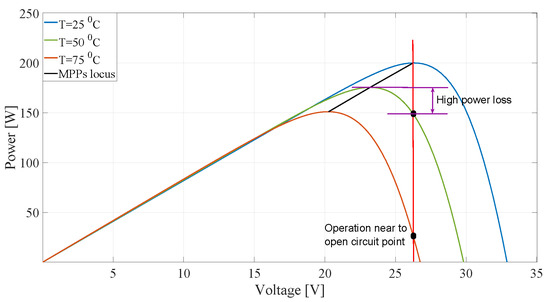
Figure 10.
MPP voltages’ variation range with different temperature conditions.
To measure the effects of radiation and temperature on the MPP location, open circuit voltage, and short circuit current methods are very common in the literature [13,15]. In these methods, the MPP is calculated as a fraction from the open circuit voltage or the short circuit current. The value of this fraction (constant) is mostly dependent on the utilized PV module’s characteristics. However, a 70%–90% range is provided in the literature [13,15]. A significant drawback of these methods is that they need to momentarily interrupt the PV power to get the values of the open circuit voltage or the short circuit current. Moreover, these interruptions are periodic to account for the atmospheric conditions’ variations. Thus, power losses and inaccuracies add to the concerns related to these methods.
So far, it is obvious that most of model-based MPPT techniques rely on radiation or temperature effects separately. Furthermore, open circuit and short circuit methods isolate the load or the grid from the PV source during calibration of the MPP’s location. Thus, concerning this gap in the model-based MPPT methods, the effects of temperature and radiation are included in this work.
As a conclusion from the last discussion, the MPP voltages’ locus should be precisely located based on the radiation and temperature variations as follows [48,50]:
where is the MPP voltage at standard test conditions (STC) (25 °C, 1000 W/m), k is a small factor that represents the effect of radiation variation on MPP voltage’s location ( [48]), G is the radiation, is the nominal radiation (1000 W/m), is the open circuit voltage temperature coefficient (provided in the data-sheet), T is the actual temperature in Kelvin, and is the nominal temperature in Kelvin (273.15 + 25).
It is quite obvious from the previous equation that locating the MPP voltage needs the knowledge of the atmospheric conditions (T, G). The temperature can be simply sensed using a low cost sensor. However, the radiation is estimated using the already measured current and voltage to sustain the simple operation of MPPT and reduce the sensing circuitry requirements. The radiation is computed based on simple but efficient estimator as [53,54]
where is the estimated radiation; is the short circuit current at STC (provided in the data-sheet); is the short circuit current temperature coefficient (provided in the data-sheet); and are the variations of the PV source current and voltage due to atmospheric conditions, and they can by calculated as
where and are the present measurements of current and voltage; and are the current and voltage at MPP. These values at STC are available on the data-sheet. However, to consider the variation of conditions. They can be updated with relatively high accuracy as follows:
where is the MPP current at STC. Furthermore, the updated short circuit current for radiation estimation is corrected as
Finally, and to limit the oscillations at steady state, an adaptive step-size is tuned as
where s is the step-size, c is a factor to be tuned, and represents the interval between the measured voltage and the MPP voltage location, which is computed as
The procedure for harnessing the maximum power from the PV source using the adaptive model-based MPPT technique is further illustrated in Figure 11. The proposed scheme has a small computational burden and it locates the MPP voltage based on accurate modeling of the PV source; thus, the drift problem can be avoided without any iterations, boundary limitations, or complicated calculations. Moreover, the actions of the proposed MPPT technique depend on the present voltage calculation; i.e., there is no need to compare the present values of voltage and current with previous measurements as in the conventional P&O; thus, the noise effect will be highly reduced using the proposed method.
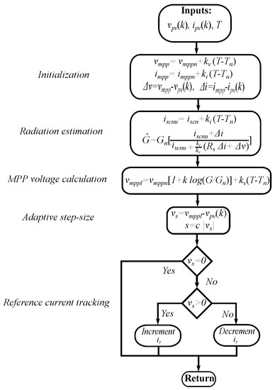
Figure 11.
The proposed adaptive model-based MPPT algorithm.
4. Dead-Beat Predictive Control for the Two-Level Inverter
The conventional control of the inverter using VOC technique requires three PI controllers, one for the outer voltage control loop and two other PI controllers for the inner current loop [29]. The present study eliminates all the PI controllers by generating the reference current for the inner loop directly from the MPPT algorithm, and hence the currents are regulated based on a dead-beat predictive function for active and reactive power management. The discrete-time model of the system for such purpose is derived by rearranging Equation (6) as follows.
Using the Euler method for forward discretization, the following results:
where is the sampling period, k is the current sampling instant, and is the predicted one. The dead-beat predictive principle assures that the predicted currents will be equal to their references at the next sampling period. Thus, substituting and instead of and , and solving the equation for reference voltages, yields
Furthermore, the predicted reference currents can be estimated using linear extrapolation as [28]
where is the previous sampling instant. Then, using Park transformation, the reference voltages in - reference frame are computed form
Finally, the calculated reference voltages are applied to space vector pulse width modulator (SVPWM) to generate the switching pulses for the two-level inverter. Figure 12 shows the whole scheme of the proposed single-stage grid-connected PV inverter, in which the adaptive MPPT provides directly the reference current for the dead-beat predictive function without the need for a PI controller. Furthermore, the reference current in q-axis direction () is set to zero to operate at unity power factor. The proposed overall control strategy is simply structured; there is no need for PI controllers tuning or predefined switching tables and constant switching frequency behavior. Besides, a fast transient response is achieved.
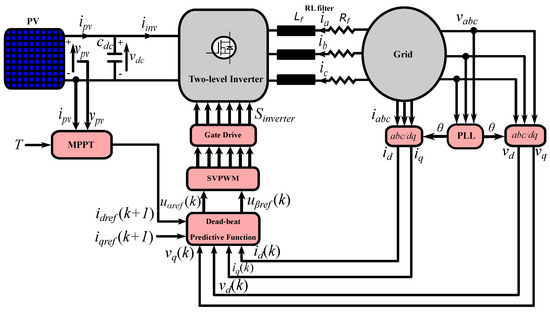
Figure 12.
The proposed control strategy for grid-connected PV inverter.
5. Simulation Results and Discussions
The proposed PV grid-connected inverter consists of a PV array of 30 kW followed by two-level inverter; a DC-link capacitor is inserted between them for coupling. Then, an RL filter is added for grid connection, as shown in Figure 12. The details of the simulated model are summarized in Table 1. The proposed adaptive model-based technique is compared with the traditional P&O method, the modified P&O with drift avoidance [23], and the multi-power-sample-based P&O algorithm [40] for investigations in various atmospheric conditions. Furthermore, and due to the coupling between MPPT and inverter control in single-stage topology, the effect of this coupling is further evaluated. Unlike most MPPT techniques, the present study investigates not only the performance of MPPT, but also its effects on the quality of the currents, power, and reactive power injected into the grid. Moreover, the drift problem impacts were checked in kind for better evaluation.

Table 1.
Parameters of the grid-connected PV system.
5.1. Performance Investigation of the Grid-Connected PV System with Radiation Variation
Various radiation profiles are used in this study to examine the efficiency of the PV system. Step changes, ramp variation, and sinusoidal profiles are used to judge the drift problem. Figure 13 shows the performances of the conventional P&O, the modified one with drift avoidance, the multi-power-sample, and the proposed adaptive model-based technique, where the radiation conditions are changed according to step variation from m to m at a constant temperature of 25 °C.
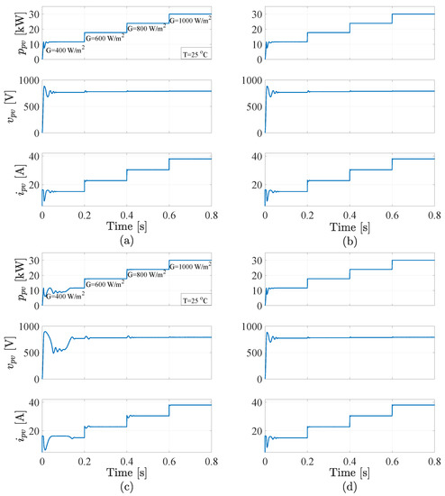
Figure 13.
MPPT performance at step changes of radiation: (a) P&O method; (b) modified P&O; (c) multi-power-sample method; (d) the proposed model-based technique.
All the MPPT techniques have excellent tracking at steady state, where the efficiency of all methods is very close, and it is about % (calculated at m and 25 °C). However, the multi-power-sample method has a slow transient behavior with step changes of the radiation, especially at start-up, as shown in Figure 13. The reason for this high value of efficiency is the high power rating of the utilized PV array (30 kW). Thus, if there are some extra ripples in range of watts in one method compared to another one, they will not be significant at this power level. This proves that testing the PV source’s efficiency with only step changes is not sufficient. Thus, the European test for efficiency (EN 50530) evaluation considers different ramp profiles with different slopes to simulate as much as possible the real atmosphere profile and to account for fast radiation change [55].
Figure 14 shows the injected active power, reactive power, d-axis current, q-axis current, and currents, respectively, when the system is operating with the conventional, modified P&O, multi-power-sample, and proposed methods.
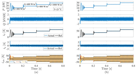
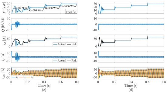
Figure 14.
Grid-connected inverter behavior at various step changes of radiation (from top): Active power injected into the grid, reactive power, d-axis current, q-axis current, and the currents for: (a) P&O method; (b) modified P&O; (c) multi-power-sample method; (d) the proposed model-based technique.
The behavior of all methods is similar. However, the transient behavior of the multi-power-sample method is a little bit slower. This slowness is inherited from the MPPT performance. The start-up of this method as shown in Figure 14 is remarkably slow; thus, a significant reactive power oscillation occurs at this period, as a result non-sinusoidal currents are injected into the grid for a long time in comparison with other methods. The ripple content of the d-axis current is smaller for the proposed model-based method, and hence the active power shows superior performance. This reflects on the THD of the injected currents, as illustrated in Table 2, where the proposed control methodology has the smallest THD among other methods.
Table 2.
THD performances of the currents with P&O, modified P&O, multi-power-sample, and the proposed method.
The drift problem appears when a gradual change in radiation happens; thus, the performance of the MPPT was studied with a ramp profile variation of radiation. Figure 15 shows the performances of P&O, modified P&O, the multi-power-sample, and the proposed method.
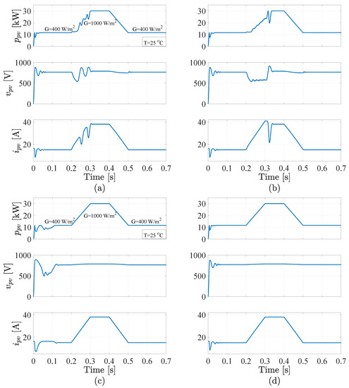
Figure 15.
MPPT performance with a ramp radiation profile: (a) P&O method; (b) modified P&O; (c) multi-power-sample method; (d) the proposed model-based technique.
As expected, the conventional P&O suffers from drift problem, where the algorithm is confused and keeps tracking in the wrong direction. The modified P&O also suffers from divergence. Furthermore, the PV voltage () has a significant drop during the ramp period. In contrast, the multi-power-sample and the proposed methods succeeded in capturing the maximum power during the gradual variation of radiation. However, the proposed model-based technique shows a better start-up performance.
The performance of the inverter control is further examined with the ramp variation of radiation. Figure 16 shows the injected active power; reactive power; d-axis current; q-axis current; and the currents, respectively, when the system operates with P&O, modified P&O, muti-power-sample, and the proposed method. As a result of the drift problem, the d-axis has very large oscillations causing the same for the active power. With P&O, the active and reactive power behavior presents enhanced performance in comparison with the modified one. The modified P&O suffers from large reactive power oscillations in conjunction with d-axis current divergence from its reference value; at the same interval the PV voltage suffers from a high voltage drop, as mentioned previously. The multi-power-sample method also suffers from some reactive power’s oscillations at start-up, whereas the proposed methodology has no oscillations, as illustrated in Figure 16.
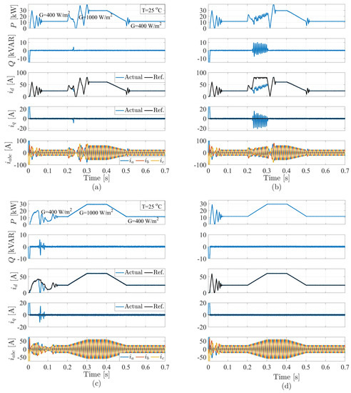
Figure 16.
Grid-connected inverter behavior with a gradual change of radiation (from top): Grid-injected active power, reactive power, d-axis current, q-axis current, and the currents for: (a) P&O method; (b) modified P&O; (c) multi-power-sample method; (d) the proposed model-based technique.
The behavior of the grid-connected PV inverter is further investigated with more complicated radiation variation for better evaluation of drift problem. A sinusoidal profile was suggested in [38], where the radiation starts with a fixed pattern, and then follows a sinusoidal one. Figure 17 shows the MPPT’s behavior of all studied methods. The P&O present some power losses due to drift. Furthermore, the PV voltage exhibits some high peaks corresponding to these losses. The modified P&O suffers from a significant power drop during the sinusoidal radiation profile, where the PV voltage shows a notable decrease.
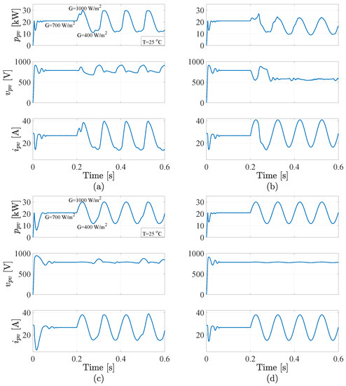
Figure 17.
MPPT performance with sinusoidal radiation change: (a) P&O method; (b) modified P&O; (c) multi-power-sample method; (d) the proposed model-based technique.
With a sinusoidal radiation profile, the multi-power-sample method presents some drift occurrence. However, it provides an enhanced performance in comparison with the conventional and modified P&O. In the case of the proposed model-based algorithm, the drift problem completely vanishes with an excellent tracking performance, as presented in Figure 17, where the power generation is smooth. Additionally, the PV voltage is limited to the maximum power region.
For obvious inspection of the MPPT behavior with gradual change of the radiation, the power–voltage portraits of the PV source are investigated for a sinusoidal profile of radiation. Figure 18 shows the power–voltage portraits for all studied MPPT methods, where the modified P&O has the widest range variation of voltage followed by P&O, then multi-power-sample method. All the three methods suffer from divergence from MPP. In contrast, the proposed model-based technique follows perfectly the MPP’s locus without any divergence, where the PV voltage is limited to the specified range according to the developed model.
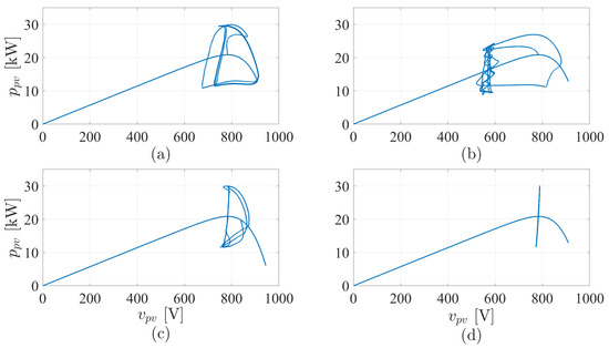
Figure 18.
Power-voltage portraits of the PV system’s MPPT with sinusoidal radiation change: (a) P&O method; (b) modified P&O; (c) multi-power-sample method; (d) the proposed model-based technique.
Furthermore, the injected active power, reactive power, d-axis current, q-axis current, and currents are illustrated in Figure 19 with P&O, modified P&O, multi-power-sample method, and the proposed technique.
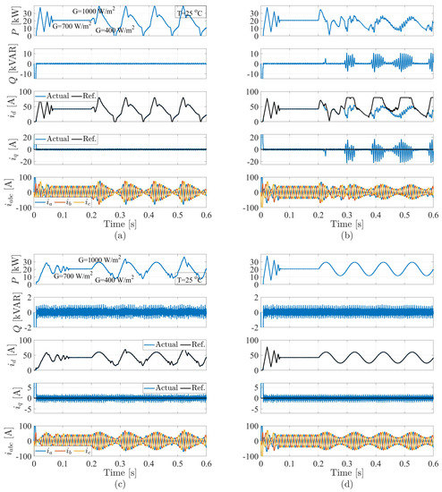
Figure 19.
Grid-connected inverter behavior with sinusoidal changes to radiation (from top): Grid-injected active power, reactive power, d-axis current, q-axis current, and the currents for: (a) P&O method; (b) modified P&O; (c) multi-power-sample method; (d) the proposed model-based technique.
With P&O, the d-axis current presents large oscillation and drops to zero, and hence the active power exhibits the same. However, the reactive power presents very good tracking. The modified P&O shows large oscillations in both active and reactive power, where the d-axis current diverts from its reference during the ascending period of the sinusoidal profile, and thus high reactive power ripples occur. As a result, non-sinusoidal currents are injected into the grid. The multi-power-sample method provides improved tracking for both active and reactive power in comparison with the P&O and the modified P&O methods. However, the d-axis current and hence the active power show some divergences inherited from the MPPT; thus, distorted sinusoidal currents are injected into the grid. The proposed technique provides the most elegant performance among the studied methods, with which excellent d-axis and q-axis current tracking were achieved. The quality of the injected active power is very high, with no drift. Furthermore, the reactive power tracking is adequate, and the injected currents are sinusoidal with low THD.
5.2. Performance of the Grid-Connected PV System with Temperature Variation
The performance of the proposed MPPT technique is further investigated with temperature variation. Figure 20 shows the performance of the MPPT at 50 °C, where the radiation is varied according to a ramp profile. The results show that the proposed technique succeeded to move the MPP in the correct direction, despite the radiation variation.
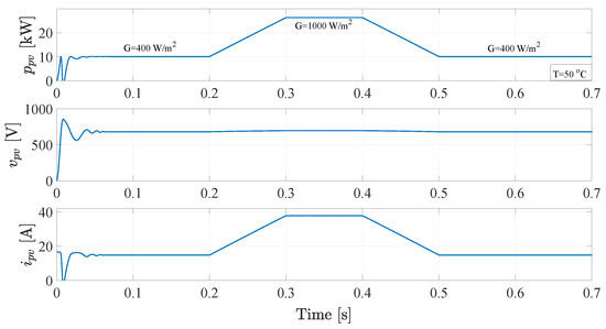
Figure 20.
MPPT performance of the proposed model-based technique at 50°C and gradual radiation change.
Moreover, the temperature was varied according to a ramp profile, where it began at 25 °C and then gradually increased to 75 °C. It is known that the temperature variation is slower than the radiation one to the degree that some authors neglect its effect. However, this condition is studied to show the effectiveness of the proposed MPPT and drift avoidance during both radiation and temperature variations. Furthermore, this was done to better evaluate the system’s performance in widely varying operation conditions, even in the worst case scenarios. The power–voltage portrait was drawn to show that the MPPT algorithm follows accurately the locus of MPPs in linear relationship, as provided in Figure 21 (see also Figure 10). Figure 21 shows that the proposed method tracks the maximum power without any drift occurrence.
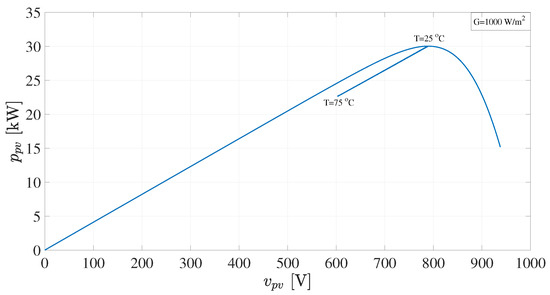
Figure 21.
Power–voltage portrait during constant radiation and gradual change of temperature.
5.3. Performance of the Grid-Connected PV System with Parameter Mismatches
The predictive dead-beat function for reference voltage generation (see Equation (18)) depends on the parameters of the system, namely, the filter resistance () and inductance (). The effect of resistance’s variation is small and can be neglected [12]. However, the inductance’s change is investigated in this subsection. The range for inductance’s variation is assumed to be .
Figure 22 presents the inverter behavior with the proposed MPPT technique at various step changes of the filter inductance. The proposed methodology maintains very good behavior in all intervals, even with low values of filter inductance. Table 3 summarizes the THD of the currents at various values of the inductance, where the highest THD value is , which is beyond the IEEE standard limitations [56] despite the mismatch. It worth mentioning that underestimating the value of the filter inductance in the model is better due to the filtering capability of the inductance, as is obvious in the intermediate interval of Figure 22.
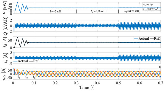
Figure 22.
Grid-connected inverter behavior at filter inductance variation (from top): active power injected into the grid, reactive power, d-axis current, q-axis current, and the currents.
Table 3.
THD of the currents for the suggested technique with variation of filter inductance.
6. Future Scope
Model-based MPPT techniques present high efficiency, even higher than most of the conventional methods [14]. Furthermore, no complex calculations are required. However, a relatively accurate model for the PV source should be used to describe the PV characteristics with high precision. It compensates for the effects of the radiation and temperature in the proposed algorithm, with limited numbers of factors for better tuning and adjusting the MPPs location. However, some key points can be inspected to further enhance the MPPT model-based algorithms; to mention a few:
- Other curve fitting tools can be utilized for accurate MPP location identification. Moreover, the data-sheet parameters as used in the proposed algorithm and experimental characteristics should be accounted for to mitigate expected deviations when working at real PV and harsh atmospheric sites.
- Investigation of the PV source parameters’ variations in the developed MPPT. The parameters of the PV source are exposed to variations due to aging and atmospheric condition changes. Thus, the MPPT should consider that issue and make sure to use factors that are most likely slow varying, while avoiding models or factors that may deteriorate the MPPT efficiency. For example, neglecting the temperature effect in the model-based MPPT techniques may lead to the operation at open circuit condition.
- Recently, monitoring of the PV source is very important to supervise online the performance of the PV system, and to expect potential faults; and to estimate the PV parameters of the PV source for the purpose of fault diagnosis. Thus, the calibration of the model-based MPPT technique can be included in the monitoring stage for MPPT enhancement and ease of operation.
- Sensorless operation—in the proposed study, the radiation is estimated using the already existing current and voltage sensors. This indeed increases the system’s reliability with cost reduction. However, a more powerful estimator can be implemented for efficiency improvement. Meta-heuristic algorithms can be combined for radiation or temperature estimation. However, the calculation burden should be taken into consideration for practical implementation. Moreover, long-term prediction techniques for atmospheric conditions can simplify the sensorless operation.
- Partial shading’s effects should be investigated on the system’s performance, as could modifying the algorithm to track the global peak to maximize the harnessed PV power.
7. Conclusions
In this paper, a detailed model of the single-stage grid-connected PV system has been proposed. The MPPT has been accomplished using a new adaptive model-based technique, where the locus of the MPPs has been located based on extensive analysis of the characteristics of the PV source at different atmospheric conditions of temperature and radiation, and thus the proposed MPPT can track the MPP location without any divergence, especially for a gradual change of radiation. The proposed technique has been compared with different techniques available in the literature for solving the drift problem. It was found, at various radiation profiles, that the developed algorithm had the most efficient performance without any drift in comparison with other methods. However, at steady state with step changes of radiation, the efficiencies of the studied MPPT techniques were very close (99.98%). Thus, the MPPT methods were evaluated based on dynamic radiation profiles, as recommended by the European efficiency test (EN 50530). Furthermore, the adaptive step reduces the oscillations around the MPP. The inverter control has been achieved with a dead-beat predictive function; thus, the cascaded loop structure of the conventional VOC was avoided. Additionally, there is no need for the outer-loop voltage controller (PI controller) associated with the conventional control techniques of the single-stage topology, as the MPPT directly generates the reference current to the inverter control; thus, the overall control strategy is simplified and the transient behavior becomes faster. The effects of the parameters’ variations on the system, specifically the inductance of the filter, have been studied. The proposed control strategy investigates the MPPT efficiency in addition to its effects on the quality of the injected currents, active power, and reactive power. As a conclusion, it is important to account for the drift problem in regions of fast atmospheric profiles. The drift problem can cause severe fluctuations of the injected active and reactive power, and hence the quality of the injected power will be deteriorated.
Author Contributions
M.A. (Mostafa Ahmed) and M.A. (Mohamed Abdelrahem) created, designed, and applied the proposed control methodology. M.A. (Mostafa Ahmed) wrote the manuscript. I.H. helped in writing and revision of the manuscript. R.K. was responsible for orientation and a number of key recommendations. All authors have read and agreed to the published version of the manuscript.
Funding
This research received no external funding.
Acknowledgments
This work was assisted by the German Research Foundation (DFG) and the Technical University of Munich (TUM) in the scope of the Open Access Publishing Program.
Conflicts of Interest
The authors report no conflict of interest.
References
- Pudukudy, M.; Yaakob, Z.; Mohammad, M.; Narayanan, B.; Sopian, K. Renewable hydrogen economy in Asia—Opportunities and challenges: An overview. Renew. Sustain. Energy Rev. 2014, 30, 743–757. [Google Scholar] [CrossRef]
- Owusu, P.A.; Samuel, A.-S. A review of renewable energy sources, sustainability issues and climate change mitigation. Cogent Eng. 2016, 3, 1167990. [Google Scholar] [CrossRef]
- Ahmed, M.; Mohamed, A.; Ralph, K.; Christoph, M.H. Maximum Power Point Tracking Based Model Predictive Control and Extended Kalman Filter Using Single Voltage Sensor for PV Systems. In Proceedings of the 2020 IEEE 29th International Symposium on Industrial Electronics (ISIE), Delft, The Netherlands, 17–19 June 2020; pp. 1039–1044. [Google Scholar]
- Zahedi, A. Maximizing solar PV energy penetration using energy storage technology. Renew. Sustain. Energy Rev. 2011, 15, 866–870. [Google Scholar] [CrossRef]
- Al-Masri, H.M.; Abu-Errub, A.; Walaa, R.A.; Mark, E. On the PV module characteristics. In Proceedings of the 2016 International Symposium on Power Electronics, Electrical Drives, Automation and Motion (SPEEDAM), Capri, Italy, 22–24 June 2016; pp. 901–905. [Google Scholar]
- Bilgili, M.; Arif, O.; Besir, S.; Ali, K. An overview of renewable electric power capacity and progress in new technologies in the world. Renew. Sustain. Energy Rev. 2015, 49, 323–334. [Google Scholar] [CrossRef]
- Taibi, E.; Dolf, G.; Morgan, B. The potential for renewable energy in industrial applications. Renew. Sustain. Energy Rev. 2012, 16, 735–744. [Google Scholar] [CrossRef]
- Hosseini, S.E.; Mazlan, A.W. Hydrogen production from renewable and sustainable energy resources: Promising green energy carrier for clean development. Renew. Sustain. Energy Rev. 2016, 57, 850–866. [Google Scholar] [CrossRef]
- Gao, F.; Ding, L.; Poh, C.L.; Yi, T.; Peng, W. Indirect dc-link voltage control of two-stage single-phase PV inverter. In Proceedings of the 2009 IEEE energy conversion congress and exposition, San Jose, CA, USA, 20–24 September 2009; pp. 1166–1172. [Google Scholar]
- Ayad, A.; Ralph, K. A comparison of quasi-Z-source inverters and conventional two-stage inverters for PV applications. EPE J. 2017, 27, 43–59. [Google Scholar] [CrossRef]
- Li, H.; Xu, Y.; Adhikari, S.; Rizy, D.T.; Li, F.; Irminger, P. Real and reactive power control of a three-phase single-stage PV system and PV voltage stability. In Proceedings of the 2012 IEEE Power and Energy Society General Meeting, San Diego, CA, USA, 22–26 July 2012; pp. 1–8. [Google Scholar]
- Ahmed, M.; Mohamed, A.; Ralph, K. Highly Efficient and Robust Grid Connected Photovoltaic System Based Model Predictive Control with Kalman Filtering Capability. Sustainability 2020, 12, 4542. [Google Scholar] [CrossRef]
- Bhatnagar, P.; Nema, R.K. Maximum power point tracking control techniques: State-of-the-art in photovoltaic applications. Renew. Sustain. Energy Rev. 2013, 23, 224–241. [Google Scholar] [CrossRef]
- De Brito, M.A.G.; Galotto, L.; Sampaio, L.P.; Melo, G.D.A.; Canesin, C.A. Evaluation of the main MPPT techniques for photovoltaic applications. IEEE Trans. Ind. Electron. 2012, 60, 1156–1167. [Google Scholar] [CrossRef]
- Verma, D.; Nema, S.; Shilya, A.M.; Dash, S.K. Maximum power point tracking (MPPT) techniques: Recapitulation in solar photovoltaic systems. Renew. Sustain. Energy Rev. 2016, 54, 1018–1034. [Google Scholar] [CrossRef]
- Sera, D.; Mathe, L.; Kerekes, T.; Spataru, S.V.; Teodorescu, R. On the perturb-and-observe and incremental conductance MPPT methods for PV systems. IEEE J. Photovolt. 2013, 3, 1070–1078. [Google Scholar] [CrossRef]
- Ahmed, M.; Abdelrahem, M.; Kennel, R.; Hackl, C.M. A robust maximum power point tracking based model predictive control and extended Kalman filter for PV systems. In Proceedings of the 2020 International Symposium on Power Electronics, Electrical Drives, Automation and Motion (SPEEDAM), Sorrento, Italy, 24–26 June 2020; pp. 514–519. [Google Scholar]
- Lashab, A.; Dezso, S.; Josep, M.G.; Lászlo, M.; Aissa, B. Discrete model-predictive-control-based maximum power point tracking for PV systems: Overview and evaluation. IEEE Trans. Power Electron. 2017, 33, 7273–7287. [Google Scholar] [CrossRef]
- Femia, N.; Petrone, G.; Spagnuolo, G.; Vitelli, M. Optimization of perturb and observe maximum power point tracking method. IEEE Trans. Power Electron. 2005, 20, 963–973. [Google Scholar] [CrossRef]
- Mei, Q.; Shan, M.; Liu, L.; Guerrero, J.M. A novel improved variable step-size incremental-resistance MPPT method for PV systems. IEEE Trans. Ind. Electron. 2010, 58, 2427–2434. [Google Scholar] [CrossRef]
- Abdelsalam, A.K.; Ahmed, M.M.; Shehab, A.; Prasad, N.E. High-performance adaptive perturb and observe MPPT technique for photovoltaic-based microgrids. IEEE Trans. Power Electron. 2011, 26, 1010–1021. [Google Scholar] [CrossRef]
- Ahmed, J.; Zainal, S. A modified P&O maximum power point tracking method with reduced steady-state oscillation and improved tracking efficiency. IEEE Trans. Sustain. Energy 2016, 7, 1506–1515. [Google Scholar]
- Killi, M.; Susovon, S. Modified perturb and observe MPPT algorithm for drift avoidance in photovoltaic systems. IEEE Trans. Ind. Electron. 2015, 62, 5549–5559. [Google Scholar] [CrossRef]
- Li, X.; Huiqing, W.; Yihua, H.; Lin, J. Drift-free current sensorless MPPT algorithm in photovoltaic systems. Solar Energy 2019, 177, 118–126. [Google Scholar] [CrossRef]
- Zeb, K.; Uddin, W.; Khan, M.A.; Ali, Z.; Ali, M.U.; Christofides, N.; Kim, H.J. A comprehensive review on inverter topologies and control strategies for grid connected photovoltaic system. Renew. Sustain. Energy Rev. 2018, 94, 1120–1141. [Google Scholar] [CrossRef]
- Hassaine, L.; Lias, E.O.; Quintero, J.; Salas, V. Overview of power inverter topologies and control structures for grid connected photovoltaic systems. Renew. Sustain. Energy Rev. 2014, 30, 796–807. [Google Scholar] [CrossRef]
- Blaabjerg, F.; Remus, T.; Marco, L.; Adrian, V.T. Overview of control and grid synchronization for distributed power generation systems. IEEE Trans. Ind. Electron. 2006, 53, 1398–1409. [Google Scholar] [CrossRef]
- Bouafia, A.; Jean-Paul, G.; Fateh, K. Predictive direct power control of three-phase pulsewidth modulation (PWM) rectifier using space-vector modulation (SVM). IEEE Trans. Power Electron. 2009, 25, 228–236. [Google Scholar] [CrossRef]
- Kadri, R.; Jean-Paul, G.; Gerard, C. An improved maximum power point tracking for photovoltaic grid-connected inverter based on voltage-oriented control. IEEE Trans. Ind. Electron. 2010, 58, 66–75. [Google Scholar] [CrossRef]
- Yang, H.; Zhang, Y.; Liang, J.; Liu, J.; Zhang, N.; Walker, P.D. Robust deadbeat predictive power control with a discrete-time disturbance observer for PWM rectifiers under unbalanced grid conditions. IEEE Trans. Power Electron. 2018, 34, 287–300. [Google Scholar] [CrossRef]
- Noguchi, T.; Hiroaki, T.; Seiji, K.; Isao, T. Direct power control of PWM converter without power-source voltage sensors. IEEE Trans. Ind. Appl. 1998, 34, 473–479. [Google Scholar] [CrossRef]
- Zhang, Y.; Li, Z.; Zhang, Y.; Xie, W.; Piao, Z.; Hu, C. Performance improvement of direct power control of PWM rectifier with simple calculation. IEEE Trans. Power Electron. 2012, 28, 3428–3437. [Google Scholar] [CrossRef]
- Rodriguez, J.; Kazmierkowski, M.P.; Espinoza, J.R.; Zanchetta, P.; Abu-Rub, H.; Young, H.A.; Rojas, C.A. State of the art of finite control set model predictive control in power electronics. IEEE Trans. Ind. Inform. 2012, 9, 1003–1016. [Google Scholar] [CrossRef]
- Cortes, P.; Rodriguez, J.; Silva, C.; Flores, A. Delay compensation in model predictive current control of a three-phase inverter. IEEE Trans. Ind. Electron. 2011, 59, 1323–1325. [Google Scholar] [CrossRef]
- Harbi, I.; Mohamed, A.; Mostafa, A.; Ralph, K. Reduced-Complexity Model Predictive Control with Online Parameter Assessment for a Grid-Connected Single-Phase Multilevel Inverter. Sustainability 2020, 12, 7997. [Google Scholar] [CrossRef]
- Vazquez, S.; Leon, J.I.; Franquelo, L.G.; Carrasco, J.M.; Martinez, O.; Rodriguez, J.; Cortes, P.; Kouro, S. Model predictive control with constant switching frequency using a discrete space vector modulation with virtual state vectors. In Proceedings of the 2009 IEEE International Conference on Industrial Technology, Churchill, Victoria, Australia, 10–13 February 2009; pp. 1–6. [Google Scholar]
- Sebaaly, F.; Hani, V.; Hadi, Y.K.; Kamal, A.-H. Novel current controller based on MPC with fixed switching frequency operation for a grid-tied inverter. IEEE Trans. Ind. Electron. 2017, 65, 6198–6205. [Google Scholar] [CrossRef]
- Ahmed, J.; Zainal, S. An improved perturb and observe (P&O) maximum power point tracking (MPPT) algorithm for higher efficiency. Appl. Energy 2015, 150, 97–108. [Google Scholar]
- Lashab, A.; Dezso, S.; Josep, M.G. A dual-discrete model predictive control-based MPPT for PV systems. IEEE Trans. Power Electron. 2019, 34, 9686–9697. [Google Scholar] [CrossRef]
- Abouadane, H.; Fakkar, A.; Sera, D.; Lashab, A.; Spataru, S.; Kerekes, T. Multiple-Power-Sample Based P&O MPPT for Fast-Changing Irradiance Conditions for a Simple Implementation. IEEE J. Photovolt. 2020, 10, 1481–1488. [Google Scholar]
- Dirscherl, C.; Christoph, H.; Korbinian, S. Modellierung und Regelung von modernen Windkraftanlagen: Eine Einführung. In Elektrische Antriebe-Regelung von Antriebssystemen; Springer: Berlin/Heidelberg, Germany, 2015; pp. 1540–1614. [Google Scholar]
- Elgendy, M.A.; Bashar, Z.; David, J.A. Assessment of perturb and observe MPPT algorithm implementation techniques for PV pumping applications. IEEE Trans. Sustain. Energy 2011, 3, 21–33. [Google Scholar] [CrossRef]
- Safari, A.; Saad, M. Simulation and hardware implementation of incremental conductance MPPT with direct control method using cuk converter. IEEE Trans. Ind. Electron. 2010, 58, 1154–1161. [Google Scholar] [CrossRef]
- Li, X.; Huiqing, W.; Lin, J.; Weidong, X.; Yang, D.; Chenhao, Z. An improved MPPT method for PV system with fast-converging speed and zero oscillation. IEEE Trans. Ind. Appl. 2016, 52, 5051–5064. [Google Scholar] [CrossRef]
- Islam, H.; Mekhilef, S.; Shah, N.B.M.; Soon, T.K.; Seyedmahmousian, M.; Horan, B.; Stojcevski, A. Performance evaluation of maximum power point tracking approaches and photovoltaic systems. Energies 2018, 11, 365. [Google Scholar] [CrossRef]
- Elgendy, M.A.; Zahawi, B.; Atkinson, D.J. Comparison of directly connected and constant voltage controlled photovoltaic pumping systems. IEEE Trans. Sustain. Energy 2010, 1, 184–192. [Google Scholar] [CrossRef]
- Liu, Y.H.; Liu, C.L.; Huang, J.W.; Chen, J.H. Neural-network-based maximum power point tracking methods for photovoltaic systems operating under fast changing environments. Sol. Energy 2013, 89, 42–53. [Google Scholar] [CrossRef]
- Ai, B.; Yang, H.; Shen, H.; Liao, X. Computer-aided design of PV/wind hybrid system. Renew. Energy 2003, 28, 1491–1512. [Google Scholar] [CrossRef]
- Abdel-Salam, M.; El-Moh, M.T.; El-Ghazaly, M. An Efficient Tracking of MPP in PV Systems Using a Newly-Formulated P&O-MPPT Method Under Varying Irradiation Levels. J. Electr. Eng. Technol. 2020, 15, 501–513. [Google Scholar]
- Yilmaz, U.; Omer, T.; Ahmet, T. Improved MPPT method to increase accuracy and speed in photovoltaic systems under variable atmospheric conditions. Int. J. Electr. Power Energy Syst. 2019, 113, 634–651. [Google Scholar] [CrossRef]
- Coelho, R.F.; Filipe, M.C.; Denizar, C.M. A MPPT approach based on temperature measurements applied in PV systems. In Proceedings of the 2010 IEEE International Conference on Sustainable Energy Technologies (ICSET), Kandy, Sri Lanka, 6–9 December 2010; pp. 1–6. [Google Scholar]
- Vicente, E.M.; Moreno, R.L.; Ribeiro, E.R. MPPT technique based on current and temperature measurements. Int. J. Photoenergy 2015, 2015, 242745. [Google Scholar] [CrossRef]
- Chikh, A.; Ambrish, C. An optimal maximum power point tracking algorithm for PV systems with climatic parameters estimation. IEEE Trans. Sustain. Energy 2015, 6, 644–652. [Google Scholar] [CrossRef]
- Moshksar, E.; Teymoor, G. Real-time estimation of solar irradiance and module temperature from maximum power point condition. IET Sci. Meas. Technol. 2018, 12, 807–815. [Google Scholar] [CrossRef]
- Ishaque, K.; Zainal, S.; George, L. The performance of perturb and observe and incremental conductance maximum power point tracking method under dynamic weather conditions. Appl. Energy 2014, 119, 228–236. [Google Scholar] [CrossRef]
- Langella, R.; Alfredo, T.; Et, A. IEEE Recommended Practice and Requirements for Harmonic Control in Electric Power Systems; IEEE: Piscataway Township, NJ, USA, 2014. [Google Scholar]


Publisher’s Note: MDPI stays neutral with regard to jurisdictional claims in published maps and institutional affiliations. |
© 2020 by the authors. Licensee MDPI, Basel, Switzerland. This article is an open access article distributed under the terms and conditions of the Creative Commons Attribution (CC BY) license (http://creativecommons.org/licenses/by/4.0/).