Abstract
The motivation for this paper is the enhanced role of power generation prediction in power plants and power systems in the smart grid paradigm. The proposed approach addresses the impact of the ambient temperature on the performance of an open cycle gas turbine when using the Kalman Filter (KF) technique and the power-temperature (P-T) characteristic of the turbine. Several Kalman Filtering techniques are tested to obtain improved temperature forecasts, which are then used to obtain output power predictions. A typical P-T curve of an open-cycle gas turbine is used to demonstrate the applicability of the proposed method. Nonlinear and linear discrete process models are studied. Extended Kalman Filters are proposed for the nonlinear model. The Time Varying, Time Invariant, and Steady State Kalman Filters are used with the linearized model. Simulation results show that the power generation prediction obtained using the Extended Kalman Filter with the piecewise linear model yields improved forecasts. The linear formulations, though less accurate, are a promising option when a power generation forecast for a small-term and short-term time window is required.
1. Introduction
Meteorological conditions affect the demand for electricity as well as the performance of the generating units, conventional or renewable [1]. Power generation prediction is important for the short-term and long-term management, operation, and planning of power systems. Over the last two decades, the need for accurate power generation forecasts has been accentuated in view of the emergent electricity markets. Accurate supply and demand forecasts are crucial, especially in the day-ahead markets where the amount of electricity to be generated needs to be predicted, in time intervals as short as 15 min, and communicated to grid operators the day before.
The accuracy of a forecasting tool depends on the model used to relate the performance of a power generating unit to meteorological parameters and the identification or training of the model with actual, current data.
The effect of parameters such as ambient air temperature and relative humidity, solar irradiance, and wind velocity on the power output of renewable energy sources has been thoroughly investigated by several researchers using both historical data and measurements and several phenomenological, statistical, or analytical models have been proposed. Though an extensive literature review on this topic is out of the scope of this paper, the effect of wind velocity on wind turbines or solar irradiation and air temperature on photovoltaics may be found in References [2,3] and references therein.
In the case of conventional power generators, the key factors affecting their performance are the technology used, (e.g., an open-cycle gas turbine, a Diesel engine, etc.), and their output dependence on operating conditions, such as the ambient air temperature, pressure, and relative humidity. Gas turbines are widely used in electricity production power systems, either in standalone mode or as a combined cycle in combination with a heat recovery steam generator and a steam turbine to generate electricity and heat for industrial processes (cogeneration) [4]. Gas turbines, especially of the aeroderivative, two spool design, are characterized by reduced installation costs and small footprint, in addition to a fast start and high ramp rates. On the other hand, gas turbines in combined cycle configurations achieve very high thermal efficiency up to 60% [5]. The shaft power output of a gas turbine is proportional to the mass flow of dry air entering the compressor. If the air volume flowrate entering the compressor is assumed to remain roughly constant for a constant speed and inlet guide vanes’ position, the air density becomes a critical factor. The air density is a function of ambient temperature, pressure, and humidity [6]. Ambient pressure variations are less pronounced at a specific location (e.g., pressure usually ranges between 990–1035 mbar, that is, ±2% over the standard atmosphere at sea level of 1013.3 mbar).
However, the ambient temperature variation can have a more significant effect, e.g., in a climate with temperatures ranging between say, −15 °C to +40 °C. In the usual two spool, aeroderivative engine design, the pressure ratio of the compressor at constant speed is reduced as the inlet temperature increases. This results in an increase of the compressor’s work, provided by the gas generator turbine, thus, leaving less net output for the power turbine. Thus, colder air results in a higher mass flow rate of air through the gas turbine, which results in an increase in shaft power output. Relative humidity is an additional factor affecting air density, since humid air contains a percentage of water vapour (which is lighter than air) that displaces an equal volume of dry air, reducing the quantity of dry air entering the engine for combustion (see the psychrometric chart for comparison [7]). However, the effect of temperature on the output involves a more complicated mechanism because the water vapour is also involved in the combustion. When lower temperature air enters the compressor, the latter’s isentropic efficiency increases. This means that the compressor consumes less power, thus, increasing the engine’s thermal efficiency (more power supplied to the generator) [8].
Gas turbine engine manufacturers have developed a variety of systems to improve engine output and efficiency and compensate the above-mentioned output losses. For example, in a two-spool aeroderivative gas turbine, the SPRINT system (Spray Intercooling) [9] injects demineralized water into the engine either upstream of the low pressure compressor or between the low pressure and high pressure compressors. In this way, air temperature is reduced by the water evaporation cooling and compressor’s efficiency increased. An alternative is evaporative cooling, which is a water fogging system that sprays a fine mist of water into the inlet air before the air filters. The cooling effect could be carried out by adsorption chillers in newer units. However, the absorption chiller is only realizable with the added complications (backpressure, etc.) of an exhaust gas recovery heat exchanger, provided that exhaust temperatures are sufficiently high.
Nevertheless, the power—temperature characteristic has the general shape of Figure 1. The net capacity of the units is given under ISO conditions (15 °C, 1 atm). This corresponds to the normalized output equal to 1 in this figure.
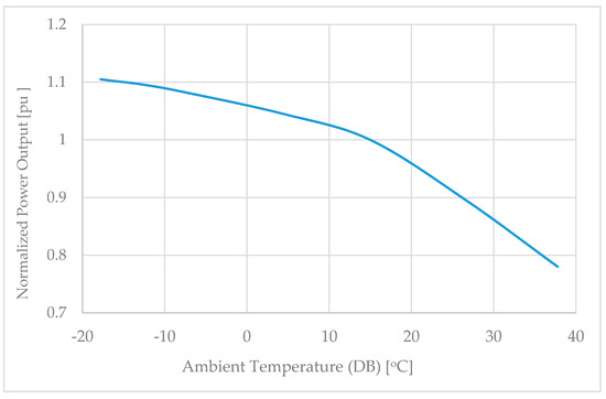
Figure 1.
The Power-Temperature characteristic of an open cycle gas turbine used in this study.
Power output may be reduced by 5% of the ISO-rated power output (15 °C, sea level) for every 10 °C increase in ambient air temperature, while the specific fuel consumption may increase by 1.5%, depending on the engine type [7].
Simple thermodynamic models of the ambient temperature effect on the output power have been proposed [10]. However, these models must be further tuned to accurately match the behavior of the specific gas turbine type and, therefore, are not widely used for output power predictions.
Instead, the Power-Temperature (P-T) characteristic provided by the manufacturer is used in conjunction with temperature forecasts based on Numerical Weather Prediction (NWP) models. This allows the plant operator to plan the production and participate in the day-ahead markets.
In any case, a more accurate temperature forecast leads to a more accurate output power prediction. Kalman Filters have been proposed for improving temperature forecasts required for predicting the amount of power generated by a gas turbine [11]. The Kalman Filter has been extensively used to obtain and improve the estimates of processes influenced by temperature variations, as in the case of SOC estimation of the batteries in electrical storage systems [12], monitoring the temperature profiles inside the heat exchangers serving an Organic Rankine Cycle (ORC) unit [13], which is power generated by gas turbines [14]. A Kalman Filter (KF) has been used for short-term temperature forecasts in Reference [14]. A one-dimensional Kalman Filter is used for the correction of near surface (2 m) air temperature forecasts obtained by an NWP model in Reference [15]. Regional weather forecasts are derived by implementing non-linear polynomial functions for different order polynomials using the Kalman Filter in Reference [16]. Ambient air temperature predictions for “sub-grid” locations that are extracted in Reference [17] using a Kalman Filter. NWP grid models suffer from systematic errors in the temperature forecast, especially at a near-ground level [16,17]. In order to reduce this drawback, local terrain topography is used for the adoption of the Kalman Filter technique in References [17,18].
This paper presents a method for power generation prediction of an open cycle gas turbine using the Kalman Filter (KF) technique [19,20] and the P-T characteristic of the turbine. A typical P-T curve of an open-cycle gas turbine is used to demonstrate the applicability of the proposed method for improved output power predictions. It also presents the derivation of the Extended Kalman Filter to be used with a non-linear discrete process model and tests the performance of Time Invariant Kalman Filters for linear or linearized models for short-term predictions and of the Steady State Kalman Filter for faster predictions.
The paper is organized as follows. Section 2 presents the general non-linear discrete process model relating the output power of an open-cycle gas turbine to ambient temperature through its non-linear P-T characteristic. A linearized model is also proposed to be used with more efficient KF formulations. In Section 3, the KF-based algorithms are presented. In Section 4, simulation results concerning the power output prediction for a given P-T curve are presented and discussed. The conclusions are summarized in Section 5.
2. Models
The general discrete time non-linear model describes the relationship between the n-dimensional state x(k) and the m-dimensional measurement z(k) at time k.
where the functions f(x(k),k) and h(x(k),k) are non-linear and w(k) and v(k) are the state and measurement noises, which are assumed to be Gaussian with constant mean values and known covariances Q(k) and R(k), respectively. The initial value of state x(0) is assumed to be a Gaussian random variable with mean x0 and covariance P0.
The non-linear is reduced to the linear model by expressing and as linear combinations of the state vector .
The above formulations are used to compute the prediction x(k + 1/k) of the state and the prediction error covariance P(k + 1/k). The prediction horizon, which, in this paper, is assumed to be 1 h, depending on the available data.
2.1. Non-Linear Model
The non-linear model is developed using information from [14,21]. The state is the power output of the gas turbine in pu and the measurement is the ambient air temperature. The non-linear model is described as follows.
Assuming that the power output changes very slowly, f(x(k),k) = F = 1 [19], and the state model of (1) reduces to (5).
The typical P-T curve of an open-cycle gas turbine may be modeled as a stepwise linear relationship, consisting of two successive linear segments.
The state noise variance Q(k) holds the values of the difference between successive values of power generation for an interval preceding the prediction time. The measurement noise variance R(k) holds the values of the difference between successive values of temperature for the previously mentioned interval. Since they are both time varying, the model is time varying.
To develop a time invariant model, the variances must assume to be constant for a fixed interval preceding the prediction time.
2.2. Linear Model
Similar to the non-linear case, the linear model is described by (8) and (9). The state is the output power of the gas turbine in p.u. based on the nominal power output at 15 °C and the measurement is the ambient air temperature.
Assuming that the power output changes very slowly, f(x(k),k) = F = 1 [19], and the state model of (1) reduces to (8).
In order to linearize the piece-wise linear P-T characteristic, h(x(k),k) is replaced by a linear function, which passes from the point of discontinuity and has a gradient equal to the mean of the gradients of the two linear segments.
where,
Then,
Again, state and measurement noise variances are time varying and concern an interval preceding the prediction time.
3. Prediction Algorithms
In this section, the prediction KF algorithms for the non-linear and the linear case are presented.
3.1. Prediction Algorithms for the Non-Linear Model
The Extended Kalman Filter (EKF) is proposed for the non-linear model. Depending on the computation of the covariance matrices Q(k) and R(k), the following two EKF algorithms are developed.
3.1.1. Extended Kalman Filter with Time-Varying Backward Time Interval b (EKF-b)
In this case, selecting a fixed time interval b (backwards) preceding the prediction time, the time varying state, and measurement noise variances are computed online. The formulation is given below.
for k = 0, 1, …, with initial conditions x(0/1) = x0, P(0/1) = P0.
3.1.2. Extended Kalman Filter with Fixed Time Interval f (EKF-f)
In this case, selecting a fixed time interval f (fixed) preceding the prediction time launch, the constant state, and measurement noise variances are computed off-line. The formulation is given below.
with the same initial conditions.
It is worth noting that, due to the form of the function h(x(k)), the above Extended Kalman Filter is equivalent to the combined use of two Time Varying Kalman Filters depending on the prediction value x(k/k − 1). The first Kalman Filter is used when x(k/k − 1) ≤ c with parameters H1 = a1, s1 = d1. The second Kalman Filter is used when x(k/k − 1) > c with parameters H2 = a2, s2 = d2. This is shown in Figure 2.
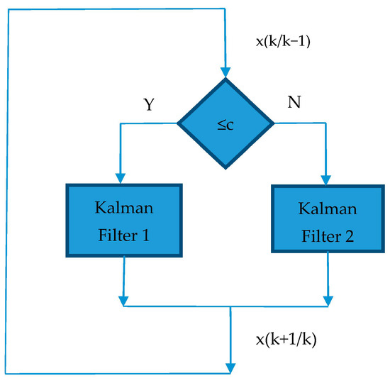
Figure 2.
The proposed Kalman Filter as equivalent to two Time Varying Kalman Filters combined.
3.2. Prediction Algorithms for the Linear Model
The Time Invariant Kalman Filter and the Steady State Kalman Filter are proposed for the linear model.
3.2.1. Time Invariant Kalman Filter with a Fixed Time Interval f (TIKF-f)
In this case, selecting a fixed time interval f (fixed) preceding the prediction time launch, the constant state and measurement noise variances are computed off-line. The formula is given below.
for k = 0, 1, …, with initial conditions x(0/1) = x0, P(0/1)=P0.
3.2.2. Steady State Kalman Filter with a Fixed Time Interval f (SSKF-f)
It is known [19] that, when the model is asymptotically stable, then there exists a steady state prediction error variance P, which depends on the constant noise variances. In this case, selecting a fixed time interval f (fixed) preceding the prediction time launch, the constant state, and measurement noise variances are computed off-line. Then, the steady state prediction error variance is also computed off-line. The formula is given below.
The parameters
are pre-calculated through the steady state gain K:
which is derived by the positive root
of the corresponding Riccati equation [19,22].
3.2.3. FIR Steady State Kalman Filter (FIRSSKF-f-ε)
Note that 0 < A < 1. In this case, the Finite Impulse Response (FIR) Steady State Kalman Filter (FIRSSKF) is developed as in Reference [23].
where
and M, such that: AM ≥ ε and AM + i < ε, i = 1,2,…, where ε is the convergence criterion.
For the computation of the FIR SSKF coefficients, the values of the noise variances and the convergence criterion ε, determining the FIR length M, are required. The constant noise variances are computed off-line for a fixed time interval f before the prediction time launch. The convergence criterion ε must be set to a value determined beforehand through trial simulations. In order to calculate the prediction, a subset of previous measurements must be provided. The method can be used in order to derive a prediction for a specific time in the future, without the need to compute any intermediate predictions.
4. Simulation Results
A typical P-T curve of gas turbines is depicted in Figure 1 and is described by the following set of parameters.
The results presented in Section 4.1 and Section 4.2 refer to an one-week time period, during which the temperature variations are presented in Figure 3. In this figure, the blue curve corresponds to the actual (measured) temperature, while the red one corresponds to the forecasted (NWP) temperatures.
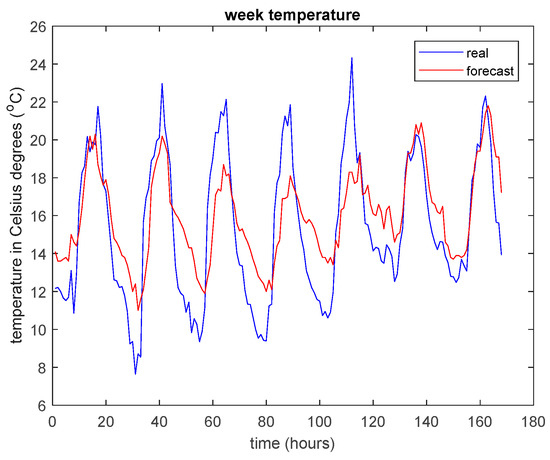
Figure 3.
Weekly temperature variation used for the tests.
All the prediction algorithms were implemented using MATLAB(v7, Mathworks). However, no specific software is required since any programming language can be used.
4.1. Simulation Results for the Nonlinear Model
EKF-b was applied for the nonlinear model for b = 2, 3, 6, with initial conditions x0 = 1, P0 = 0.1. The parameter b does not affect the filters’ efficiency, since the percent Mean Absolute Error (%MAE) is 1.4399%, 1.4709%, and 1.5739%, respectively.
EKF-f was applied for the nonlinear model for f = 168 (1 week) and f = 720 (1 month) with the same initial conditions. The parameter f does not affect the filters’ efficiency since the percent Mean Absolute Error (%MAE) is 1.6604% and 1.6905%, respectively.
Figure 4 depicts the output power prediction, using EKF-b with b = 3 and EKF-f with f = 720. The actual power as provided by the P-T curve for actual temperature measurements, the power forecast as obtained from the P-T curve based on the NWP forecast temperature, and the predicted power by EKF are plotted for one week (168 h). The proposed KF algorithms reproduce the trend of the actual power generation curve and the results are, in general, closer to the actual power than the output power forecast based on the NWP forecast temperature.
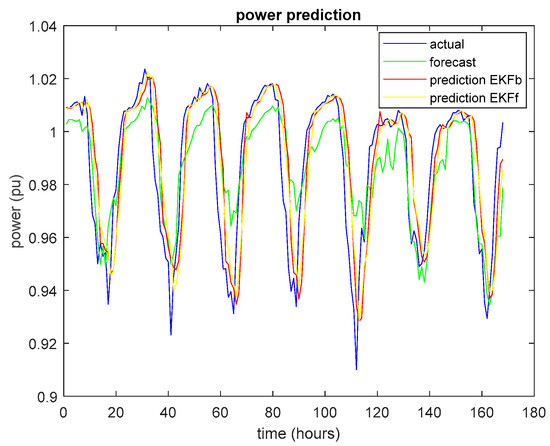
Figure 4.
Power generation prediction with the Extended Kalman Filter (EKF) using the nonlinear model.
In addition, it has been shown that the EKF in the nonlinear case presented here is equivalent to two Time Varying Kalman Filters (TVKFs). The output power predicted using EKF-b with b = 3 and EKF-f with f = 720, on the one hand, and the combination of two TVKFs, on the other hand, are compared in Figure 5. The actual power, the power forecast according to the NWP model, and the predicted power by EKF and two TVKFs are plotted for one week (168 h). The algorithms provide equivalent predictions.
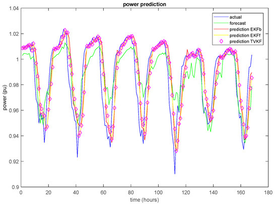
Figure 5.
The Extended Kalman Filter is equivalent to two Time Varying Kalman Filters combined.
4.2. Simulation Results for the Linear Model
TIKF-f and SSKF-f have been applied in the case of the linear model with the same initial conditions, and f = 168 (1 week), f = 720 (1 month). Both algorithms compute predictions very close to each other, since the percent Mean Absolute Error (%MAE) is 2.4240% for TIKF-f and 2.4233% for SSKF-f, for f = 720.
Figure 6 depicts the ouput power prediction, using TIKF-f and SSKF-f with f = 720. The actual power as provided by the P-T curve for actual temperature measurements, which is the power forecast as obtained from the P-T curve based on the NWP forecast temperature, and the predicted power by TIKF and SSKF are plotted for 1 week (168 h). The proposed KF algorithms reproduce the trend of the actual power generation curve and the results are generally closer to the actual power than the output power forecast based on the NWP forecast temperature.
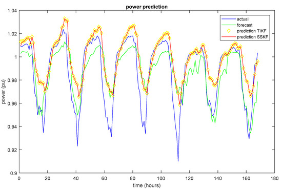
Figure 6.
Power generation prediction with the Kalman Filter (KF) using the linear model.
FIRSSKF-f-ε was applied in the case of the nonlinear model for f = 168 (1 week) and f = 720 (1 month). Several values for the convergence criterion ε were used: . The value of ε does not affect the filters’ efficiency, but it affects the FIR length M, since M = 5 for , M = 3 for .
Figure 7 depicts the results for the output power prediction when FIRSSKF-f-ε is used with f = 720 and (M = 5) and (M = 3). The actual power as provided by the P-T curve for actual temperature measurements, the power forecast as obtained from the P-T curve based on the NWP forecast temperature, and the predicted power by SSKF with FIR length M = 3 and M = 5 are plotted for 1 week (168 h).The proposed KF algorithms reproduce the trend of the actual power generation curve and the results are generally closer to the actual power than the output power forecast based on the NWP forecast temperature. It is confirmed that the FIR length does not affect the filters’ efficiency.
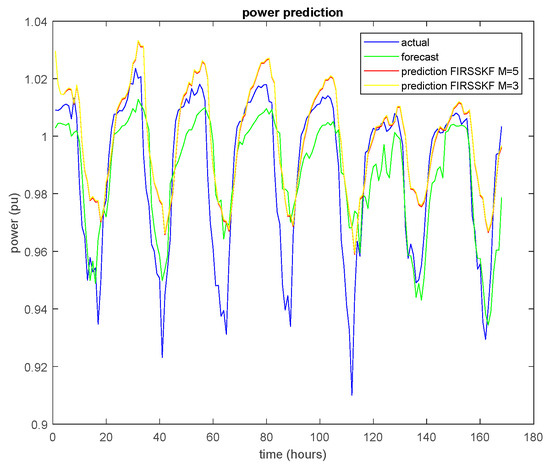
Figure 7.
Power generation prediction with FIRSSKF using the linear model.
In addition, it was confirmed that SSKF and FIRSSKF compute predictions very close to each other. The results for the power prediction, using SSKF and FIRSSKF with f = 720 and are depicted in Figure 8. The actual power, the power forecast according to the NWP model, and the predicted power by SSKF and FIRSSKF are plotted for one week (168 h). The algorithms provide similar predictions.
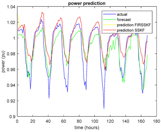
Figure 8.
SSKF is equivalent to FIRSSKF.
Figure 9 shows the comparison of all KF implementations against output power calculated based on actual and forecasted temperature profiles. Results are shown for the power generation prediction for one week (168 h), using EKF, TIKF, and SSKF with b = 3, f = 720, . All algorithms perform well and follow the general trend of the actual power generation curve offering an improved prediction compared to the power forecast based on the NWP temperature forecast. This is especially the case for the EKF implementations, which manage to capture the sharp decrease in output power for temperature local maxima.
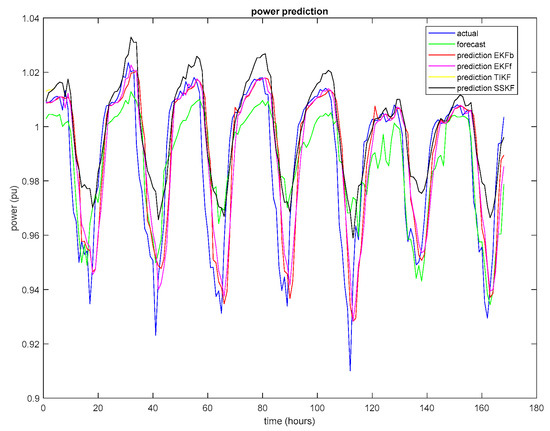
Figure 9.
Power generation prediction with KF.
4.3. Prediction Algorithms Performance
The following metrics are used to evaluate the performance of the prediction algorithms.
where the prediction error for each time is defined as the difference between the Kalman Filter prediction for the output power and the actual output power .
Table 1 presents the efficiency of the algorithms with repect to these metrics. It summarizes the results obtained by the implementation of the prediction algorihtms using EKF, TIKF, SSKF, and FIRSSKF with b = 3, f = 720, and for a one-month time period.

Table 1.
Efficiency of KF prediction algorithms used in output power prediction.
From Table 1, it is clear that the Extended Kalman Filters provide power predictions of high accuracy, significantly improved for all the metrics over those obtained using the NWP temperature forecast. More specifically, for the EKF, it was found that: (a) the Mean Bias Error (MBE) is 0.0017, (b) the Mean Absolute Error (MAE) is 0.0139, (c) the % Mean Absolute Error (% MAE) is 1.4709%, (d) the Mean Squared Error (MSE) is 0.0004, (e) the Root Mean Squared Error (RMSE) is 0.0191, and (f) the % Root Mean Squared Error (% RMSE) is 2.0388%.
Additionally, we propose the use of two more metrics.
The percent prediction improvement (% PI) with respect to power forecast, which is used to assess the improvement offered by the proposed method against the one based on NWP temperature forecasts.
where is the number of improved predictions and is the number of observations. A prediction is improved when , where is the forecast and is the forecast error.
The percent successful prediction (% SP), which is used to assess the validity of the proposed approach.
where is the number of successful observations and is the number of observations. According to the European Center for Medium-Range Weather Forecasts (ECMWF), a successful temperature forecast entails an absolute error of less than 2 °C. Assuming that, for each successful temperature forecasted, we obtain a successful power output forecast, the number of successful predictions is obtained.
Table 2 presents the effectiveness of the prediction algorithms with respect to these two metrics. It summarizes the results obtained by the implementation of the prediction algorihtms using EKF, TIKF, SSKF, and FIRSSKF with b = 3, f = 720, for a one-month period of time.
Table 2.
Effectiveness of KF prediction algorithms used in output power prediction.
From Table 2, it is clear that the Extended Kalman Filters provide output power predictions of high effectiveness. More specifically, for the EKF, it was found that: (a) the Prediction Improvement of output power prediction with respect to output power based on the NWP temperature forecast is of the order of 65%, and (b) the successful prediction of power generation is of the order of 73.33%.
5. Conclusions
Accurate power generation predictions are important in the planning and operation of a power plant as well as for efficient market bidding.
The Extended Kalman Filter (EKF), Time Invariant Kalman Filter (TIKF), and Steady State Kalman Filter (SSKF) have been used to predict the ouput power of an open cycle gas turbine given its characteristic nominal power-temperature curve, rather than using the NWP temperature forecast.
Nonlinear as well as linear discrete process models describing the power generation with respect to temperature have been presented.
The EKF was formulated for the nonlinear model. The derived algorithms are time varying. For the case presented here, the EKF is equivalent to the combination of two Time Varying Kalman Filters. TIKF and SSKF have been derived for the linear model. The derived algorithms are time invariant and simple to implement. TIKF and SSKF produce predictions very close to each other. Furthermore, the FIR implementation of the Steady State Kalman Filter needs a subset of previous time measurements to calculate a predicted value while there is no need to calculate intermediate predictions.
The choice of Kalman Filter parameters does not significantly affect the filters’ efficiency: b = 3 h, f = 168 h (= 1 week), and are proposed.
The performance and efficiency of the EKF, TIKF, and SSKF algorithms have been compared for the same P-T curve, actual (observed), and forecasted temperature data for a given week, computing several metrics, such as the percent mean absolute error, the percent improvement of power prediction with respect to the power forecast, and the percent successful prediction. The output power prediction with respect to the power forecast is improved, when the absolute difference between the predicted and the actual output power is less than the absolute difference between the actual power and that obtained using the NWP temeprature forecast. EKF produces the best predictions compared to all other algorithms, with a % Mean Absolute Error (%MAE) of the order of 1.5% and successful predictions of the power generation of the order of 73%.
Future work will focus on using the proposed methodology to predict the output power of a gas turbine by taking into account ambient pressure and relative humidity measurements.
Author Contributions
Conceptualization, C.M., N.A., and A.K. Methodology, C.M., N.A., and V.V. Software, N.A. and V.V. Validation, C.M., T.S., and V.V. Formal analysis A.K. and T.S. Investigation, C.M., A.K., and T.S. Resources, N.A. and C.M. Data curation, V.V. and T.S. Writing—original draft preparation, N.A. and V.V. Writing—review and editing, C.M., A.K., and T.S. Visualization, C.M., A.K., and T.S. Supervision, C.M. Project administration, N.A. All authors have read and agreed to the published version of the manuscript.
Funding
This research received no external funding.
Conflicts of Interest
The authors declare no conflict of interest.
References
- Teisberg, T.J.; Weiher, R.F.; Khotanzad, A. The Economic Value of Temperature Forecasts in Electricity Generation. Bull. Am. Meteorol. Soc. 2005, 86, 1765–1772. [Google Scholar] [CrossRef]
- Angelopoulos, A.; Ktena, A.; Manasis, C.; Voliotis, S. Impact of a Periodic Power Source on a RES Microgrid. Energies 2019, 12, 1900. [Google Scholar] [CrossRef]
- Roumpakias, E.; Stamatelos, A. Comparative performance analysis of grid-connected photovoltaic system by use of existing performance models. Energy Convers. Manag. 2017, 150, 14–25. [Google Scholar] [CrossRef]
- Haglind, F. A review on the use of gas and steam turbine combined cycles as prime movers for large ships. Part III: Fuels and emissions. Energy Convers. Manag. 2008, 49, 3476–3482. [Google Scholar] [CrossRef]
- González-Díaz, A.; Alcaráz-Calderón, A.M.; González-Díaz, M.O.; Méndez-Aranda, Á.; Lucquiaud, M.; González-Santaló, J.M. Effect of the ambient conditions on gas turbine combined cycle power plants with post-combustion CO2 capture. Energy 2017, 134, 221–233. [Google Scholar] [CrossRef]
- Baakeem, S.S.; Orfi, J.; Alaqel, S.; AlAnsary, H. Impact of Ambient Conditions of Arab Gulf Countries on the Performance of Gas Turbines Using Energy and Exergy Analysis. Entropy 2017, 19, 32. [Google Scholar] [CrossRef]
- Dos Santos, A.P.P.; Andrade, C.R. Thermodynamic Analysis of Gas Turbine Performance With Different Inlet Air Cooling Techniques. In ASME Turbo Expo GT2012; ASME: Copenhagen, Danmark, 2012; pp. 79–89. ISBN 978-0-7918-4474-8. [Google Scholar]
- Kurz, R.; Brun, K. Gas Turbine Performance—What Makes The Map? In Proceedings of the 29th Turbomachinery Symposium, Houston, TX, USA, 18–21 September 2000. [Google Scholar]
- GE. Spray Intercooling (SPRINT) Performance Augmentation. 1998. Available online: https://www.ge.com/power/gas/gas-turbines/lm6000 (accessed on 10 August 2020).
- Mohapatra, A.K. Analysis of parameters affecting the performance of gas turbines and combined cycle plants with vapor absorption inlet air cooling. Int. J. Energy Res. 2014, 38, 223–240. [Google Scholar] [CrossRef]
- Vikias, V.; Manasis, C.; Ktena, A.; Assimakis, N. Forecasting for Temperature Dependent Power Generation Using Kalman Filtering. In Proceedings of the IEEE 60th International Scientific Conference on Power and Electrical Engineering of Riga Technical University (RTUCON), Riga, Latvia, 7–9 October 2019. [Google Scholar]
- Pierobon, L.; Schlanbusch, R.; Kandepu, R.; Haglind, F.; Haglind, F. Application of Unscented Kalman Filter for Condition Monitoring of an Organic Rankine Cycle Turbogenerator. In Proceedings of the 2014 Annual Conference of the Prognostics and Health Management Society, Fort Worth, TX, USA, 27 September–3 October 2014. [Google Scholar]
- Auger, F.; Hilairet, M.; Guerrero, J.M.; Monmasson, E.; Orlowska-Kowalska, T.; Katsura, S. Industrial Applications of the Kalman Filter: A Review. IEEE Trans. Ind. Electron. 2013, 60, 5458–5471. [Google Scholar] [CrossRef]
- Giunta, G.; Vernazza, R.; Salerno, R.; Ceppi, A.; Ercolani, G.; Mancini, M. Hourly weather forecasts for gas turbine power generation. Meteorol. Z. 2017, 26, 307–317. [Google Scholar] [CrossRef]
- Galanis, G.; Anadranistakis, M. A one-dimensional Kalman filter for the correction of near surface temperature forecasts. Meteorol. Appl. 2002, 9, 437–441. [Google Scholar] [CrossRef]
- Galanis, G.; Louka, P.; Katsafados, P.; Pytharoulis, I.; Kallos, G. Applications of Kalman filters based on non-linear functions to numerical weather predictions. Ann. Geophys. 2006, 24, 2451–2460. [Google Scholar] [CrossRef]
- Lynch, C.; Mahony, M.J.O.; Guinee, R.A. Accurate day ahead temperature prediction using a 24 h Kalman filter estimator. In Proceedings of the 11th Conference on Ph.D. Research in Microelectronics and Electronics (PRIME), Glasgow, UK, 29 June–2 July 2015. [Google Scholar]
- De Carvalho, J.R.P.; Assad, E.D.; Pinto, H.S. Kalman filter and correction of the temperatures estimated by PRECIS model. Atmos. Res. 2011, 102, 218–226. [Google Scholar] [CrossRef]
- Anderson, B.D.O.; Moore, J.B. Optimal Filtering; Dover Publications: New York, NY, USA, 2005. [Google Scholar]
- Kalman, R.E. A New Approach to Linear Filtering and Prediction Problems. J. Basic Eng. 1960, 82, 35–45. [Google Scholar] [CrossRef]
- Welch, G.; Bishop, G. An Introduction to Kalman Filter. 2006. Available online: https://www.cs.unc.edu/~welch/media/pdf/kalman_intro.pdf (accessed on 8 June 2020).
- Lainiotis, D.; Assimakis, N.D.; Katsikas, S. Fast and numerically robust recursive algorithms for solving the discrete time Riccati equation: The case of nonsingular plant noise covariance matrix. Neural Parallel Sci. Comput. 1995, 3, 565–583. [Google Scholar]
- Assimakis, N.; Adam, M. FIR implementation of the Steady-State Kalman Filter. Int. J. Signal Imaging Syst. Eng. 2008, 1, 279–286. [Google Scholar] [CrossRef]


Publisher’s Note: MDPI stays neutral with regard to jurisdictional claims in published maps and institutional affiliations. |
© 2020 by the authors. Licensee MDPI, Basel, Switzerland. This article is an open access article distributed under the terms and conditions of the Creative Commons Attribution (CC BY) license (http://creativecommons.org/licenses/by/4.0/).