Abstract
The work presents a heat transfer analysis carried out with the use of COMSOL Multiphysics software applied to a new solar concentrator, defined as the Compound Parabolic Concentrator (CPC) system. The experimental measures have been conducted for a truncated CPC prototype system with a half-acceptance angle of 60°, parabola coefficient of 4 m−1 and four solar cells in both covered and uncovered configurations. These data are used to validate the numerical scenario, to be able to use the simulations for different future systems and works. The second challenge has been to change the reflector geometry, the half-acceptance angle (60° ÷ 75°) and the parabola coefficient (3 m−1 ÷ 6 m−1) to enhance the concentration of sun rays on the solar cells. The results show that the discrepancy between experimental data and COMSOL Multiphysics (CM) have led to validate the scenarios considering the average temperature on the solar cells. These scenarios are used for the parametric analysis, observing that the optimal geometry for the higher power and efficiency of the whole system is reached with a lower half-acceptance angle and parabola coefficient.
1. Introduction
International awareness about renewable energy sources exploitation has been changing over the last years, as a consequence of both climate changes and increasing pollution emissions [1,2]. The increasing demands of energy for industrial production and urban facilities ask for new strategies for energy sources [3]. Many industrial and private efforts have been implemented to reduce the anthropic impact on nature, trying to move from a petroleum-based fuel dependency to a new virtuous approach, also based on biomass exploitation. Possible examples are the use of fuel cells [4], biomass gasification system aimed at hydrogen production [5], combined gas conditioning and cleaning in biomass gasification [6], waste vegetable oil transesterification [7], hydrogen production from biomass [8], biofuel [9], biogas production from poultry manure and cheese whey wastewater [10], greenhouses with photovoltaic modules [11], oriented to the green economy and to the sustainable development of society [12,13]. The solar energy source should be considered as a possible solution to face the fossil-fuel exploitation to produce thermal and electric energy [14,15], using for example photovoltaic systems [16,17] with also energy storage [18] or solar collectors [19]. Photovoltaic (PV) systems manufacturers are pushing the scientific research to work on solar radiation concentrators, which should be considered as both a short-term and economic solution if compared to the production of improved semi-conductive layers and materials. Concentrator photovoltaics (CPV) is a photovoltaic technology that generates electricity from sunlight. Sun rays can be concentrated on the solar cell with various types of concentrators: lens concentrator, mirror concentrator, reflector concentrator, static concentrator, Luminescent Solar Concentrator [20,21]. Systems using low-concentration photovoltaics (LCPV) have the potential to become competitive in the near future with low cost. Reflector concentrators’ family is a kind of LCPV, and the Concentrator Parabolic Compound (CPC) is one of the most studied. The geometry of the CPC is important to convey the sun’s incoming beam and diffuse radiation in the desired receiver as much as possible [22] to increase the power output from CPC-based photovoltaic systems, particularly in recent years as discussed by authors of [23,24,25,26,27,28,29,30]. Over the past 50 years, many researches have been working with CPCs to improve solar cell efficiency [23,31], studying the geometry of most variations of concentrators [32,33] according to principles of edge-ray and identical optical path determining the profile of its reflector [34,35]. Under non-concentrating conditions, the efficiency of the solar cells drops slightly as the temperature of the cells gradually increases [27,36]. This temperature increase becomes prominent under concentration and a further drop in efficiency is observed under high solar rays concentration [37]. On the other hand, for a CPC-based photovoltaic module, the power output should increase by a factor that depends on its geometric concentration as compared to a similar non-concentrating PV panel [35]. In those terms, a multi-physical numerical simulation approach should be considered very suitable for this kind of application, allowing the implementation of virtual scenarios by which different investigation analysis could be conducted [38,39,40,41,42].
This work aims to define the temperature field within a Compound Solar Concentrator (CPC) prototype for a daily operational time, by solving a 3D transient Finite Element Method simulation scenario validated with the experimental data acquired by Trinity College Dublin (TCD). Then, a parametrisation is used to change the geometric parameters of the reflectors (half-acceptance angle and parabola coefficient) observing the solution with the higher radiative total heat flux through the solar cells and efficiency of the whole system.
2. Materials and Methods
2.1. Experimental Characterisation
The aim of this work is to obtain the temperature fields on CPC solar cells surfaces, focusing on the average temperature. The experimental campaign was conducted by considering two different exposures to the external environment: the first acquisition was conducted by installing the CPC provided with a side and upper cover, which define the covered configuration, on a roof as reported in Figure 1a, where an air volume remains trapped within the closed CPC; the second acquisition was conducted once both side and upper covers were removed (to obtain the uncovered CPC system configuration), as shown in Figure 1b, exposing the whole components to the external convection.
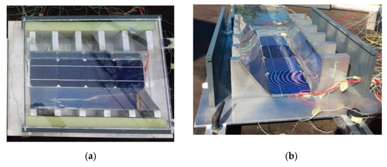
Figure 1.
Compound Parabolic Concentrator (CPC) prototypes installation: (a) covered CPC system; (b) uncovered CPC system.
The whole monitoring and data acquisition system is reported in Figure 2, where some RTDs should be noticed. The structure closed to the left side of the CPC is a reference configuration of solar cells, where no compound parabolic concentrator was installed: such reference has been used to define the efficiency of the solar cells when no concentrator is used. In fact, the experimental campaign has been conducted to define the electrical behaviour of PV cells simultaneously to the temperature acquisitions. The used MUX switching unit is an Agilent 3472A LXI data logger, installed to detect output voltage and current from the CPC and from the reference system, to compare both electrical efficiencies and highlight the CPC-related improvements. Twelve K-type thermocouples were fixed on both CPC systems, and a pyranometer was used to measure the solar incident radiation. An insulated box from Campbell Scientific Ltd. (Logan, UT, USA) was installed in order to host the electric circuit, the data logger, and two 220 V power supply plugs.
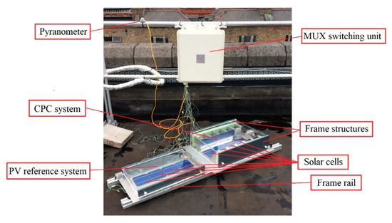
Figure 2.
Data monitoring and acquisition system setup for the experimental campaign: reference system on the left, CPC system on the right.
The experimental campaign was conducted on the aforementioned CPC configurations in 2017 on the roof of Simon Perry’s building at Trinity College Dublin, Ireland, South-oriented. Experimental data for numerical scenario validation are taken by [43], considering two days of characterisation with similar external conditions to compare the configurations. In fact, the data for the covered CPC system are referred to 17 July 2017 while for the uncovered one to 18 July 2017. The temperature distribution on the solar cells surfaces of the CPC systems is summarised in Table 1, for the covered and uncovered CPC systems. Only the solar cells have been considered to validate numerical data since the acquired temperature values from other components should not be consistent for this specific purpose due to the adopted sampling procedure.

Table 1.
Solar cells average temperature on surfaces for the covered CPC system (17 July 2017 and 18 July 2017) [43].
The temperature on the solar cells influences its efficiency since these parameters are inversely proportional; for the solar cell, the module efficiency decreases with temperature typically of −0.2%/K up to −0.5%/K [15]. Therefore, it is important to check and monitor the temperature in the system. Furthermore, to validate the functioning of the concentrator, a comparison between a simple PV and CPC system was conducted by Trinity College Dublin. The maximum values achieved on 17 July 2017 for different hours are reported in Table 2. The temperatures were obtained by a visual analysis of the graphs reported by an author in [43]. The values must be considered as rounded to the nearest whole number. Due to the numerical approximation, such resolution of temperature values is considered as suitable for simulation purposes. The data reported in tables are those validated and used in the numerical simulations.
Table 2.
Maximum values on 17 July 2017 for photovoltaic (PV) and CPC configurations [43].
2.2. Main Physical Phenomena Identification and Implementation
To ensure the multi-physical approach by validated interfaces, COMSOL Multiphysics (CM) was chosen as the most suitable FEM-based software (Finite Element Method) to implement the numerical scenario. The main phenomena analysed with CM were the heat transfer dynamics, once a surface-to-surface radiation interface had been coupled with the convective—due to external environment convection—and conductive—between the components in contact within the CPC system—heat transfer modelling. Whenever radiation heat flux is significant, the emissivity of each surface has to be considered, since this parameter measures the quantity of the incident radiation that will be emitted by the target. Moreover, the emissivity itself could depend strongly upon the wavelength of the radiation, and upon the treatment, the same surface was submitted to. The analytic problem of the radiative heat flux is described by the following equation:
where [m] is the wavelength from which emissivity [] depends, [W/(m2K4)] is the Stephan-Boltzmann constant, [K] is the surface temperature, and [K] is the ambient temperature. Referring to an example given by CM [44], let’s consider the fraction of total emitted power as a function of wavelength for a black body at different temperatures (5800 K considering the Sun and a 500 K reference temperature for most of the engineering cases). The wavelength of 2.5 μm could divide the solar spectral band (closely similar to that of a 5800 K black body) from the ambient one, where the peak of 500 K black body’s emitted power is located. The solar radiation absorbed by the grey body has a wavelength less than 2.5 μm, while re-radiation to the surroundings is emitted from a wavelength value of 2.5 μm. It highlights the need to define within the pre-processing interface the emissivity of the generic material for the domain of the solar spectral band and for that of the ambient spectral band. By setting up the simulation, the user should insert two values of emissivity, that is for the solar spectral band () and for the ambient spectral band (). The total incoming radiative flux at a specific point is the irradiation [W/m2], while the outgoing radiative flux is defined as radiosity [W/m2], according to the COMSOL manual [45]. The radiosity should be considered as the sum of both reflected and emitted radiations by the target surface. Considering those quantities analytically, this is the definition:
where [], , [W/m2] and denote the reflectivity of surface, its emissivity, the blackbody total emissive power and the temperature, respectively. In addition to the concept of absorptivity and emissivity, the view factor [] has to be defined, as it plays an important role in defining the exposure to radiation between the involved surfaces. This factor depends only of the radiating bodies geometry [46] since the emitting radiation from surface is intercepted by surface . It follows the definition of the view factor
where [W/m2] is the radiative heat flux that goes from surface to surface , and is the total radiative heat flux emitted by . Each part of the geometry should be characterised by a specific view factor referring to all the other parts of the geometric domain: CM assigns those factors automatically. The Sun position is computed automatically by the built-in feature in CM, once latitude, longitude, time zone, date, and time are given. The solar radiation direction is defined by a specific method similar to the one exposed by the author in [47]. The zenith angle () and azimuth angle () of the Sun are converted into a direction vector in Cartesian coordinates assuming that the north, the west, and the up directions correspond to the x, y, and z directions, respectively (refer to Figure 3).
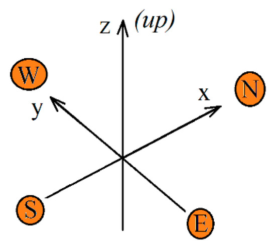
Figure 3.
North (N), South (S), East (E), and West (W) in COMSOL Multiphysics (CM) for solar irradiance direction.
2.3. Simulation Campaign
The strategy of the simulation campaign is based on experimental data obtained at Trinity College Dublin with the acquisition system setup, as reported in Figure 2. Data have been conducted for the covered and uncovered CPC systems on 17 and 18 July 2017, respectively. With these data and geometry known, modelling and numerical simulations are carried out. Three-dimensional models are built in CM for the covered and uncovered configurations. For the numerical scenarios, the inputs are the environmental conditions (solar radiation and temperature in a day of the year) and general assumptions, since the weather is considered as a random phenomenon. For each component, the materials are assigned with a bibliography analysis to find a correct value for both solar and spectral emissivity (main condition in solar radiation phenomenon defining). One of the critical steps for the numerical simulation is the boundary definition, understanding how and which conditions have to be implemented to obtain a reality-comparable scenario. The mesh is realised once the physic phenomenon and the modelling procedure of it are known, to achieve both convergence and consistent results. Finally, the post-processing is conducted, analysing the thermal fields in the configurations and using the results to study the thermal response of the CPC systems. The computed scenarios have been checked to fit experimental results. In this way, there is the possibility to understand the behaviour of CPCs in various ambient conditions, monitoring the temperature fields and other CPCs systems’ characteristics. The simulation campaign is resumed by the flow chart in Figure 4.
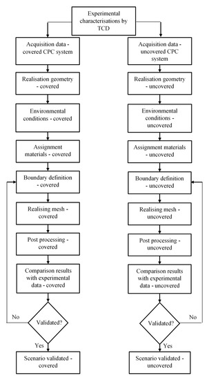
Figure 4.
Flow chart of simulation campaigns.
The part in COMSOL Multiphysics begins with the realisation of the CPC system geometry using the built-in model geometry builder. The measures and dimensions are referred to the prototype realised by Trinity College Dublin as described by the author of [43], the reconstruction of the inner components of the whole CPC system are reported in Figure 5.
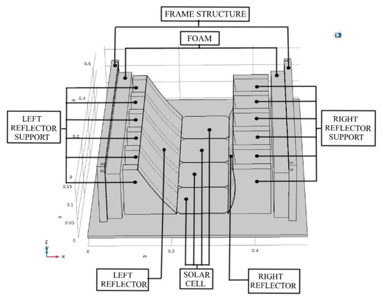
Figure 5.
Inner components of the whole CPC system.
In the simulation campaigns, the geometrical model is cut with a symmetry plane to decrease the computational time and the required hardware resources. The built model is shown in Figure 6.
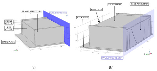
Figure 6.
External components of a covered CPC system symmetry model: (a) back view; (b) symmetry plane view.
To solve the modelling of the CPC system, it is necessary to know the environmental conditions, the temperature, and solar radiation for 17 and 18 July 2017 from 0:00 to 23:30. A daily temperature trend has been obtained from the Dublin Airport Weather Station [48], as plotted in Figure 7.
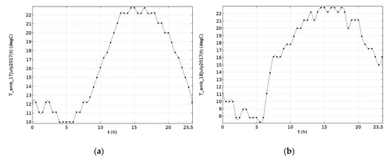
Figure 7.
Ambient temperature of: (a) 17 July 2017; (b) 18 July 2017.
The data of solar radiation is taken by the CMAS Radiation Service web-page [49]. For the simulation scenario, the subdivision of the beam and diffuse radiation component is very important: clear sky BHI (Beam Horizontal Irradiation) and clear sky DHI (Diffusive Horizontal Irradiation). The measurement of daily solar radiation is plotted in Figure 8.
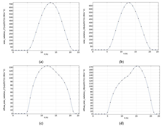
Figure 8.
Solar radiation subdivision: (a) Beam Horizontal Irradiation (BHI) on 17 July 2017; (b) BHI on 18 July 2017; (c) DHI on 17 July 2017; (d) DHI on 18 July 2017.
A specific material was assigned to each component in the simulation scenario, as described in Table 3. The parameters have been obtained by literature [43,50,51,52,53,54].
Table 3.
Materials’ properties assigned to each domain.
The boundary conditions have been imposed to solve the heat transfer dynamics with surface-to-surface radiation in the CPC systems where the external radiation source is implemented to define the directional radiation source. The source is the Sun position, and its influence is linked to the location of the studied system, once coordinates, date, and local time are given. On the one hand, all the parts radiated by the sun are diffuse surfaces; they reflect radiative intensity uniformly in all direction with a run-time computed view factor. On the other hand, the reflectors are considered diffuse mirrors because the surfaces are characterised by emissivity values around zero. To reduce the calculation time, the symmetry condition is applied by dividing the geometry model into two equal parts with a cutting symmetry plane, and the thin layer condition is applied to define the solar cells surfaces. The heat flux feature adds a convective flux to the external surfaces; the condition used is the wind velocity. A preliminary study to validate the scenarios determines a wind velocity of 0.5 m/s. Then the models are meshed and calculated with a transient study from 05:00 to 18:00 on 17 July 2017 and 18 July 2017 for the covered and uncovered configuration, respectively. The discretisation is shown in Figure 9a,b, respectively.
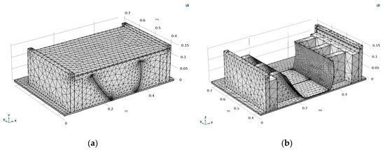
Figure 9.
Final mesh adopted for each configuration of the CPC model: (a) covered; (b) uncovered.
Details about the implemented mesh characteristics for both CPC configurations are listed in Table 4.
Table 4.
Mesh characteristics for both CPC configurations.
The simulations output is the transient 3D thermal field all over the domains of the CPC, which should be used to focus on the maximum temperatures once reached by the solar cells. Post-processing of numerical results is conducted to calculate:
- The efficiency of the solar cells following the examples provided by authors in [55,56,57];where is the solar cell surface temperature and is the solar irradiance, both time dependent, is the efficiency in standard condition (17.5%), is the temperature coefficient (0.0045 K−1), and is the solar radiation coefficient (0.12). It should be noticed that the solar irradiance term needs to be divided by the reference solar irradiance (1000 W/m2), since Equation (4) could result in the once standard irradiance conditions are given (25 °C, 1000 W/m2);
- The radiative total heat flux through the solar cell n.2, useful to understand the output power available for the photovoltaic system;
- The efficiency of the whole system. This efficiency considers the presence of the reflectors that convey the sun’s rays on the solar cells, increasing the solar radiation concentration. The value is calculated by the equation derived by experimental data
Once the scenarios have been validated, a parametric analysis is conducted to carry out a wider analysis. It is possible to quickly evaluate the most suitable configuration against a much greater range of real-word scenarios, that would be possible through physical prototyping, saving up time and costs once using the validated simulation scenario as an investigation tool. The chosen parameters to carry out the parametric analysis are related to the geometry of the reflectors, needed to convey incoming beam and diffuse radiation in the desired receiver as much as possible [22]. The schematic diagram of the CPC is shown in Figure 10. The shape of the reflectors is the same for both configurations.
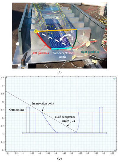
Figure 10.
Realisation of reflectors geometry: (a) main parts of reflectors construction, (b) 2D scheme of the CPC system.
The reflectors are built by a left parabola with a vertical symmetry axis (white dashed line in Figure 10a, characterised by a coefficient of 4 m−1. By the other hand, the right reflector of the system is built with a right parabola with the same coefficient but rotated like it is possible to see its symmetry axis (white dashed inclined line). The angle between the symmetry axis is the half-acceptance angle: it indicates how much the right parabola is rotated. For this specific prototype, the half-acceptance angle is equal to 60°. The point of intersection between the left parabola and the symmetry axis of the right parabola (the yellow circle in Figure 10a determines the height of truncation of the CPC system. The chosen geometrical parameters are:
- a, which is the coefficient that appears in the parabola definition formula and indicates the parabola concavity;
- Half-acceptance angle: indicates the rotation of the right parabola, which is the angle between the symmetry axis of the left and right parabola, as shown in Figure 10.
These two geometrical parameters affect the opening of the reflector and the conveying of the sun rays on the solar cells. CM allows to carry out a parametric sweep combining the parameters chosen in all possible combinations given by Table 5.
Table 5.
Parametric sweep combination.
The description of the considered values could be the following:
- The range of a chosen is from 3 to 6 m−1 to compare the results with different parabola shapes, the opening of the parabola is greater with higher values;
- The range of half-acceptance angle chosen is from 60° (the angle of the previously calculated scenario) because the system has the bound of width, with a lower angle than 60°, the opening of the parabola is greater, and the geometry construction is not feasible.
The influence of the half-acceptance angle and parabola coefficient on geometry is shown in Figure 11, reporting the extremal geometrical parameter combinations effects on the geometry appearance.
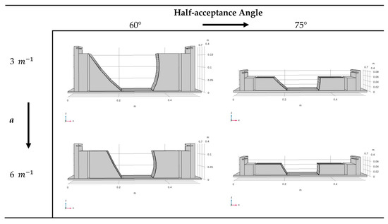
Figure 11.
Influence of half-acceptance angle and parabola coefficient on geometry.
It is possible to observe that with the same parabola coefficient, increasing the half-acceptance angle results in a decrease in terms of the CPC system height. Similar effect should be noticed while increasing the parabola coefficient. Therefore, for each CPC system, n.16 scenarios are computed to define the average temperature of the only solar cell n.2, since the centre area of the CPC is characterised by a higher temperature and so is more critical. From these data, post-processing of numerical results is conducted by plotting:
- Maximum radiative total heat flux through the solar cell n.2, calculated for each combination of sweep parameters;
- Maximum efficiency of the whole system calculated for each combination of sweep parameters. With this result it is possible to know which configuration is better to convey the sun rays on the beam. In fact, the aim of the reflector is to obtain a higher power on the solar cell to convert it into electricity. This efficiency considers the presence of the reflectors that convey the sun rays on the solar cells, increasing the concentration. The value is calculated by Equation (5).
3. Results
3.1. Numerical Scenarios Validation
The first step is the validation of the scenarios comparing the results obtained by numerical simulation (from COMSOL Multiphysics) with the ones by experimental campaigns [43]. The temperature field on the surfaces exposed to the external environment conditions is reported in Figure A1 and Figure A2 for the covered and uncovered configuration for the validation of the scenario, respectively, by which the influence of external convection condition is highlighted on the frame structures, back plate, and covers. Considering the aim of this work, a specific view of the temperature distribution on the reflectors and the solar cells surfaces is also reported in Figure A3 and Figure A4, for the covered and uncovered configuration, respectively. The temperature daily trend on the solar cells for the covered and uncovered CPC configuration is reported in Figure 12a,b, respectively.
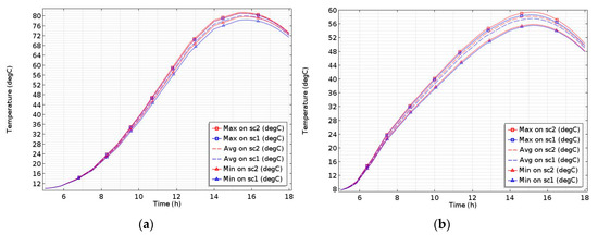
Figure 12.
Temperature trend on the solar cells: (a) covered CPC system (17 July 2017); (b) uncovered CPC system (18 July 2017).
The maximum, average, and minimum values of the surface temperature over time are computed for both configurations. These graphs show that it is possible to consider the average temperature on the solar cell n.2 as a representative thermal parameter of the whole system: the difference between maximum and minimum temperature values over time is less than 3.0 °C, which indicates a uniform temperature distribution along the solar cell surfaces. The temperature peaks for both configurations occur at around 15:00 with 80 °C and 55 °C, respectively. This important difference is due to the covers that trap the air in the system, increasing the temperature. The trends follow the incident solar radiation during the day where the extremal hours can be influenced by external factors. After obtaining the temperature values, the post-processing analysis has been conducted to plot the efficiency of solar cells n.1 and n.2, as reported in Figure 13a,b for the covered and uncovered configuration, respectively, once Equation (4) has been used. It refers to the portion of energy that can be converted via photovoltaics into electricity by solar cells, obtained from the only temperature measured on the surfaces. Therefore, this efficiency indicates how the solar cells work, but it does not take into account the whole electrical devices that are connected to the cells. In Figure 13, it is possible to see that the efficiency on the solar cells in the uncovered configuration is higher because the temperature is lower for the cooling effect of the air to which the system is exposed directly.
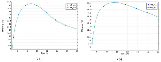
Figure 13.
Efficiency of the solar cells over time: (a) covered CPC system (17 July 2017); (b) uncovered CPC system (18 July 2017).
A complete analysis of the CPC system can be obtained studying the radiative heat flux through the solar cell n.2, plotted in Figure 14. By this way it is possible to understand the role of the reflectors in conveying the incident solar radiation on the solar cells, increasing then the convertible solar energy into electrical energy.
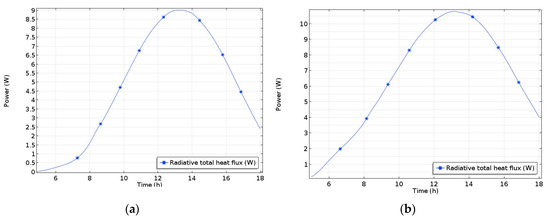
Figure 14.
Radiative total heat flux through the solar cell n.2: (a) covered CPC system (17 July 2017); (b) uncovered CPC system (18 July 2017).
The incident solar radiation peaks for the covered and uncovered configuration reach 9 W and 11 W, respectively, obtained both at around 13:00. The trends faithfully follow the incident solar radiant of input where the extremal values can be influenced by external factors. The difference between configurations is about 2 W due to the covers that attenuate the incoming rays. Then, it is possible to obtain the efficiency of the whole system using Equation (5). In this case, the efficiency is influenced by the presence of the reflectors while conveying the sun rays on the solar cells. The results are shown in Figure 15. The trends are similar to the radiative total heat flux plots, reaching peaks of efficiency of about 18% and 22% for the covered and uncovered configuration, respectively.
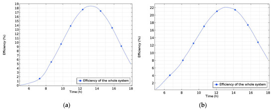
Figure 15.
Efficiency of the whole systems: (a) covered CPC system (17 July 2017); (b) uncovered CPC system (18 July 2017).
The validation of numerical data is conducted by comparing it with experimental data. To validate the numerical scenarios, the percentage discrepancy parameter is used as described by the following equation:
The temperatures are reported in Table 6 for the covered and uncovered configuration, reporting the single discrepancies for each couple of data (experimental and numerical). The discrepancies in the peak of temperature (around hour 15:00) are very low; it is important this overlapped because this value can be used in the phase of electrical analysis.
Table 6.
Comparison of solar cells average temperature on surfaces for the covered and uncovered CPC system by experimental characterisation (TCD) and numerical simulation (CM) with relative discrepancy.
Calculating the global discrepancy, the values obtained for the two configurations are: 10.4% and 7.7% for the covered and uncovered one, respectively. The limit for the validation of the results has been imposed by 12.0% discrepancy, due to the technical issues while implementing external convection conditions that should be the same of real-life external environments. Under these conditions, both systems can be validated.
Furthermore, the post-processing results are compared with the experimental ones to validate the scenarios; the radiative total heat flux through the solar cell n.2 is shown in Table 7, the efficiency of the whole system in Table 8.
Table 7.
Comparison of the radiative total heat flux for the covered CPC system by experimental characterisation (TCD) and numerical simulation with relative discrepancy (CM) (17 July 2017).
Table 8.
Comparison of efficiency in the whole system for the covered CPC system by experimental characterisation (TCD) and numerical simulation with relative discrepancy (CM) (17 July 2017).
The global discrepancies are 1.6% and 2.4% for the radiative total heat flux and efficiency of the whole system, respectively. By that, the post-processing results validate the numerical scenarios.
3.2. Parametric Analysis
The parametric analysis is conducted changing the reflector geometry: the half-acceptance angle and the parabola coefficient. The aim is to observe the better configuration for higher sun rays concentration. The average temperatures of solar cell n.2 over time are shown in Figure 16a–d and Figure 16e–h for the covered and uncovered configuration, respectively. In each graph there are different trends of temperature for various half-acceptance angles (60° ÷ 75°), once the parabola coefficient has been fixed between the range 3 m−1 ÷ 6 m−1. For the covered configuration, the average temperature on solar cell n.2, considering different parabola coefficient, is imperceptible by an engineering point of view, while in the same figure the trends of different half-acceptance angle are not overlapped. On the other hand, for the uncovered configuration, the temperature has been changing, being influenced by both the parabola coefficient and half-acceptance angle, observing that the maximum temperature decreases while decreasing these two parameters.
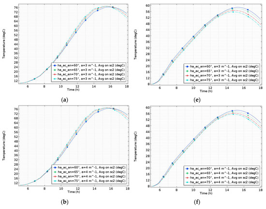
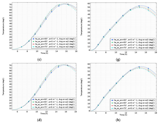
Figure 16.
Temperature on solar cell n.2 with different half-acceptance angles and parabola coefficients for the: (a–d) covered CPC system; (e–h) uncovered CPC system.
Post-processing analysis is conducted to characterise the system and to identify the most suitable solution to enhance the solar radiation concentration on the solar cells. The radiative total heat flux through solar cell n.2 is plotted in Figure 17 for both configurations. It is used to understand how much the reflectors geometry conveys the sun rays. The peaks of power are plotted for each parametric combination of parabola coefficient and half-acceptance angle. The maximum values are obtained for lower parabola coefficient and half-acceptance angle for the geometry construction, considering 3 m−1 and 60°, respectively. The difference between uncovered and covered configuration, while considering the aforementioned combination of parabola coefficient and half-acceptance angle, is about 1.8 W due to the presence of the covers that attenuates the incident solar radiation. For the covered one (Figure 17a), the influence of the parabola coefficient and half-acceptance angle on the power output appears to be similar. For the uncovered configuration (Figure 17b), the half-acceptance angle shows a major influence on the incident heat flux (multiplied by the surface of the cells) if compared to the influence of the parabola coefficient.
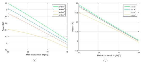
Figure 17.
Maximum radiative total heat flux through solar cell n.2 for different half-acceptance angles and parabola coefficients: (a) covered CPC system; (b) uncovered CPC system.
The efficiency of the whole system is calculated by means of Equation (5), referring to the portion of energy as the sun’s incident radiation, that can be converted by means of PV plant into electricity. The maximum values of the whole systems efficiency for each combination are reported in Figure 18 for both covered and uncovered configuration. The system shows a higher efficiency with lower parabola coefficient and half-acceptance angle. A difference of about 3.5%, considering the most performing combination of the parabola coefficient and half-acceptance angle between configurations, could be noticed in terms of whole system efficiency.
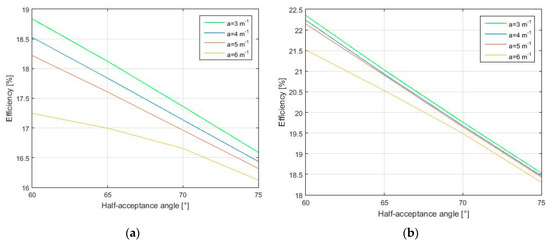
Figure 18.
Maximum efficiency of the whole system for different half-acceptance angles and parabola coefficients: (a) covered CPC system; (b) uncovered CPC system.
4. Discussion
The numerical temperature results fit the expected values by experimental campaigns. On the one hand, the uncovered CPC configuration appears to reach the best performance in terms of cooling, since a maximum temperature of around 55 °C is reached on the solar cells surface, as shown in Figure 12b. The trend follows the sun curve of radiation, with the maximum at hour 15:00. On the other hand, the characteristics of the solar cell structures and frames impose the installation of a cover to prevent any damage or deposition of particles on the critical surfaces, that could lead to many losses in terms of efficiency. However, considering the covered configuration, a temperature of around 80 °C is reached on the solar cells surfaces, as shown in Figure 12a at hour 15:00. Once analysing the typical dependence of PV cell electric efficiency on the semiconductor temperature, it should be noticed in Figure 13 how the uncovered configuration guarantees higher efficiency of the solar cells than the covered one. The use of reflector increases the solar incident radiation on the PV cell, improving the photogeneration of charge carriers but meanwhile, increases the temperature. Another important parameter is the radiative total heat flux through solar cell n.2 because it allows to understand the correct conveying of the sun rays. Higher incoming solar radiation power corresponds to major conversion into electricity by the photovoltaic effect. The difference between the covered and the uncovered configuration should be highlighted by the power peaks of about 9 W and 11 W, respectively, as shown in Figure 14. The trend is like the solar radiation, with the maximum at hour 13:00. The reason of difference between values is the presence of an internal air domain that attenuates the solar radiation in the case of covered configuration. Furthermore, the maximum efficiency of the whole system has been estimated around 18.3% and 22.0% for the covered and uncovered configuration, respectively, as plotted in Figure 15. The validation of the scenarios is conducted calculating the discrepancy for temperature, power, and efficiency of the whole system data. In all these cases the values are below the imposed limit (12%); therefore, the numerical simulations can be considered validated. Additionally, the discrepancies during the peaks (around hour 15:00) are very low, these values are used to characterise the system. To optimise the concentration of the sun rays on the solar cells, the parametrisation of the geometrical reflectors has also been conducted. For both configurations (covered and uncovered) the reflector shape influence on CPC’s thermal response has been investigated: the varying parameters are the half-acceptance angle (60° ÷ 75°) and parabola coefficient (3 m−1 ÷ 6 m−1). The chosen parameters are bounded by the width of the system because a bigger system leads to higher costs of fabrication and more encumbrance for the installation. The results show that for the covered configuration (Figure 16a–d) the combination trends of the average temperature on the solar cell n.2 are overlapped because of the air volume presence, which remains trapped between the covers. The same air volume seems to influence the whole system efficiency negatively, since it attenuates the effect of the enhanced solar radiation concentrator on electricity production. Furthermore, for the covered configuration the curves of efficiency remain very similar for different angles and coefficients. For the uncovered configuration it is possible to see in Figure 16e–h how the higher temperature is reached for the lower half-acceptance angle (60°) and parabola coefficient (3 m−1). Post-processing analysis is used to understand the functioning of the reflector. For the power analysis, the covered configuration reaches lower values than the uncovered one because of the presence of the covers that attenuates the solar radiation. Moreover, analysing the parametric sweep, the output power increases with a lower half-acceptance angle and parabola coefficient (trend similar to the temperature one), reaching about 9.2 W and 10.9 W for the covered and uncovered configuration, respectively, as shown in Figure 17. A similar analysis is conducted observing the higher value of efficiency, obtained with a lower half-acceptance angle and parabola coefficient reaching about 18.9% and 22.4% for the covered and uncovered system, respectively, as plotted in Figure 18. Therefore, by using the global efficiency, it is possible to identify the better solution, that is a reflector built with a half-acceptance angle of 60° and a parabola coefficient of 3 m−1 for the uncovered configuration, achieving also a lower temperature on the solar cell if compared to the covered one. It leads to an improvement in terms of photogeneration of charge carriers.
5. Conclusions
The convenience in using Compound Solar Concentrators is strictly related to the improvements in terms of efficiency of the whole system. In this manuscript, the type of concentrator studied is the Compound Parabolic Concentrator (CPC) that conveys the sun rays on the solar cells. The characteristics of the prototypes realised by TCD are with the half-acceptance angle of 60° and parabola coefficient of 4 m−1. The analysis shows that the 3D transient Finite Element Method simulation scenarios for the covered and uncovered configuration can be considered validated with the experimental data acquired by Trinity College Dublin in terms of temperature, power, and efficiency of the whole system. The method used for the validation is the calculation of the average discrepancies between data: the values are below the imposed upper limit of 12%. The results show that the best performing configuration is the uncovered one since the temperature on the solar cells is lower for the effect of cooling by air. Furthermore, without covers, the incoming solar radiation on the cells is higher, not being attenuated. Then, a parametrisation of the reflectors is conducted to obtain a geometry that conveys as many rays as possible. The studied combinations are solved for a half-acceptance angle 60° ÷ 75° and for the parabola coefficient 3 m−1 ÷ 6 m−1. The results show that the optimal geometry for the higher power and efficiency of the whole system is reached with a lower half-acceptance angle and parabola coefficient. It is the first step for further works to improve this technology. Further studies and works on this technology of solar concentrators should be related to:
- Simulative campaigns conducted through a virtual laboratory, to check the influence of varying conditions on the CPC efficiency and to find a right matching of geometrical parameters to achieve the optimisation of the whole system;
- Numerical analysis and simulation of integrated cooling systems. The goal is to decrease the temperature in the system, improving the efficiency of the CPCs, removing the produced heat by means of different possible solutions. The heat should be re-used in various applications as a trigenerative ORC (Organic Rankine Cycle) system, to generate domestic hot water, for an HVAC (Heating, Ventilation, and Air Conditioning) plan or for general-purpose heating systems, according to the reached temperature value;
- The validated scenario with experimental data should be used for new CPC numerical simulations, involving different geometry, components, and a number of solar cells, avoiding the production of any physical prototype of a compound solar concentrator.
Author Contributions
Conceptualization, M.C. and S.J.M.; data curation, S.J.M., A.M., M.R. and A.O.; methodology, Maurizio Carlini, A.M. and M.R.; supervision, M.C. and S.M.; visualization, A.M., M.R. and A.O.; writing—review and editing, S.C., A.M. and M.R. All authors have read and agreed to the published version of the manuscript.
Funding
This research received no external funding.
Conflicts of Interest
The authors declare no conflict of interest.
Appendix A
The figures in the Appendix show the temperature distribution on all and part of the CPC systems, for the covered and uncovered configuration. These results are obtained with the same simulation campaign of the manuscript. Referring to the boundary conditions, the temperature fields in Figure A1, Figure A2, Figure A3 and Figure A4 are obtained by the same simulations discussed above. They could be helpful to visualise the thermal response of the system while exposed to the time-dependent conditions reported in Figure 7 and Figure 8, where temperature and solar radiation are given, respectively. Figure A3 reports the temperature field on the critical surfaces of the system, that is solar cells and reflectors. As discussed before, the maximum temperature reached by the covered scenario is higher than the one reached by the uncovered system because of the presence of the trapped air volume. Convection phenomena are much more relevant on the uncovered system since it improves the cooling of the whole structure, exposed to the external environment, directly.

Figure A1.
Temperature field on the whole surfaces of the assembly for the covered CPC scenario (17 July 2017) at the following times: (a) 10:00; (b) 11:00; (c) 12:00; (d) 13:00; (e) 14:00; (f) 15:00.
Figure A1.
Temperature field on the whole surfaces of the assembly for the covered CPC scenario (17 July 2017) at the following times: (a) 10:00; (b) 11:00; (c) 12:00; (d) 13:00; (e) 14:00; (f) 15:00.


Figure A2.
Temperature field on the whole surfaces of the assembly for the uncovered CPC scenario (18 July 2017) at the following times: (a) 10:00; (b) 11:00; (c) 12:00; (d) 13:00; (e) 14:00; (f) 15:00.
Figure A2.
Temperature field on the whole surfaces of the assembly for the uncovered CPC scenario (18 July 2017) at the following times: (a) 10:00; (b) 11:00; (c) 12:00; (d) 13:00; (e) 14:00; (f) 15:00.


Figure A3.
Temperature field on solar cells and reflectors surfaces for the covered CPC scenario (17 July 2017) at the following times: (a) 10:00; (b) 11:00; (c) 12:00; (d) 13:00; (e) 14:00; (f) 15:00.
Figure A3.
Temperature field on solar cells and reflectors surfaces for the covered CPC scenario (17 July 2017) at the following times: (a) 10:00; (b) 11:00; (c) 12:00; (d) 13:00; (e) 14:00; (f) 15:00.


Figure A4.
Temperature field on solar cells and reflectors surfaces for the uncovered CPC scenario (18 July 2017) at the following times: (a) 10:00; (b) 11:00; (c) 12:00; (d) 13:00; (e) 14:00; (f) 15:00.
Figure A4.
Temperature field on solar cells and reflectors surfaces for the uncovered CPC scenario (18 July 2017) at the following times: (a) 10:00; (b) 11:00; (c) 12:00; (d) 13:00; (e) 14:00; (f) 15:00.

References
- Nejat, P.; Jomehzadeh, F.; Taheri, M.M.; Gohari, M.; Muhd, M.Z.A. A global review of energy consumption, CO2 emissions and policy in the residential sector (with an overview of the top ten CO2 emitting countries). Renew. Sustain. Energy Rev. 2015, 43, 843–862. [Google Scholar] [CrossRef]
- Bhattacharya, M.; Paramati, S.R.; Ozturk, I.; Bhattacharya, S. The effect of renewable energy consumption on economic growth: Evidence from top 38 countries. Appl. Energy 2016, 162, 733–741. [Google Scholar] [CrossRef]
- Carlini, M.; Castellucci, S. Efficient energy supply from ground coupled heat transfer source. In Lecture Notes in Computer Science (including Its Subseries Lecture Notes in Artificial Intelligence and Lecture Notes in Bioinformatics); Springer: New York, NY, USA, 2010; Volume 6017, pp. 177–190. [Google Scholar]
- Pumiglia, D.; Vaccaro, S.; Masi, A.; McPhail, S.J.; Falconieri, M.; Gagliardi, S.; della Seta, L.; Carlini, M. Aggravated test of Intermediate temperature solid oxide fuel cells fed with tar-contaminated syngas. J. Power Sources 2017, 340, 150–159. [Google Scholar] [CrossRef]
- Pallozzi, V.; Di Carlo, A.; Bocci, E.; Villarini, M.; Foscolo, P.U.; Carlini, M. Performance evaluation at different process parameters of an innovative prototype of biomass gasification system aimed to hydrogen production. Energy Convers. Manag. 2016, 130, 34–43. [Google Scholar] [CrossRef]
- Pallozzi, V.; Di Carlo, A.; Bocci, E.; Carlini, M. Combined gas conditioning and cleaning for reduction of tars in biomass gasification. Biomass Bioenergy 2018, 109, 85–90. [Google Scholar] [CrossRef]
- Carlini, M.; Castellucci, S.; Cocchi, S. A Pilot-Scale Study of Waste Vegetable Oil Transesterification with Alkaline and Acidic Catalysts. Energy Procedia 2014, 45, 198–206. [Google Scholar] [CrossRef]
- Moneti, M.; Di Carlo, A.; Bocci, E.; Foscolo, P.U.; Villarini, M.; Carlini, M. Influence of the main gasifier parameters on a real system for hydrogen production from biomass. Int. J. Hydrogen Energy 2016, 41, 11965–11973. [Google Scholar] [CrossRef]
- Hassan, M.H.; Kalam, M.A. An overview of biofuel as a renewable energy source: Development and challenges. Procedia Eng. 2013, 56, 39–53. [Google Scholar] [CrossRef]
- Carlini, M.; Castellucci, S.; Moneti, M. Biogas Production from Poultry Manure and Cheese Whey Wastewater under Mesophilic Conditions in Batch Reactor. Energy Procedia 2015, 82, 811–818. [Google Scholar] [CrossRef]
- Carlini, M.; Villarini, M.; Esposto, S.; Bernardi, M. Performance analysis of greenhouses with integrated photovoltaic modules. In Lecture Notes in Computer Science (including Its Subseries Lecture Notes in Artificial Intelligence and Lecture Notes in Bioinformatics); Springer: New York, NY, USA, 2010; Volume 6017, pp. 206–214. [Google Scholar]
- Carvalho, H.; Govindan, K.; Azevedo, S.G.; Cruz-Machado, V. Modelling green and lean supply chains: An eco-efficiency perspective. Resour. Conserv. Recycl. 2017, 120, 75–87. [Google Scholar] [CrossRef]
- Carlini, M.; Castellucci, S.; Mennuni, A.; Ferrelli, S.; Felicioni, M.A. Application of a circular & green economy model to a ceramic industrial district: An Italian case study. In Proceedings of the AIP Conference Proceedings 2123, Xiamen, China, 17 July 2019; Volume 020087. [Google Scholar]
- Solar Energy Perspectives; International Energy Agency: Paris, France, 2011; Volume 9789264124.
- McCormack, S.J. PV Systems & Solar Thermal Systems. In Solar to Chemical Energy Conversion: Theory and Application (Lecture Notes in Energy); Sugiyama, M., Fujii, K., Nakamura, S., Eds.; Springer: New York, NY, USA, 2016. [Google Scholar]
- Carlini, M.; Honorati, T.; Castellucci, S. Photovoltaic greenhouses: Comparison of optical and thermal behaviour for energy savings. Math. Probl. Eng. 2012, 2012. [Google Scholar] [CrossRef]
- Mosconi, E.M.; Carlini, M.; Castellucci, S.; Allegrini, E.; Mizzelli, L.; di Trifiletti, M.A. Economical assessment of large-scale photovoltaic plants: An Italian case study. In Lecture Notes in Computer Science (including Its Subseries Lecture Notes in Artificial Intelligence and Lecture Notes in Bioinformatics); Springer: New York, NY, USA, 2013; Volume 7972, pp. 160–175. [Google Scholar]
- Akbari, H.; Browne, M.C.; Ortega, A.; Huang, M.J.; Hewitt, N.J.; Norton, B.; McCormack, S.J. Efficient energy storage technologies for photovoltaic systems. Sol. Energy 2019, 192, 144–168. [Google Scholar] [CrossRef]
- Hegarty, R.O.; Kinnane, O.; McCormack, S.J. Parametric investigation of concrete solar collectors for façade integration. Sol. Energy 2017, 153, 396–413. [Google Scholar] [CrossRef]
- Rafiee, M.; Chandra, S.; Ahmed, H.; McCormack, S.J. An overview of various configurations of Luminescent Solar Concentrators for photovoltaic applications. Opt. Mater. 2019, 91, 212–227. [Google Scholar] [CrossRef]
- Rafiee, M.; Ahmed, H.; Chandra, S.; Sethi, A.; McCormack, S.J. Monte Carlo Ray Tracing Modelling of Multi-Crystalline Silicon Photovoltaic Device Enhanced by Luminescent Material. In Proceedings of the 2018 IEEE 7th World Conference on Photovoltaic Energy Conversion (WCPEC) (A Joint Conference of 45th IEEE PVSC, 28th PVSEC & 34th EU PVSEC, Waikoloa Village, HI, USA, 10–15 June 2018; pp. 3139–3141. [Google Scholar]
- Kessentini, H.; Bouden, C. Numerical and experimental study of an integrated solar collector with CPC reflectors. Renew. Energy 2013, 57, 577–586. [Google Scholar] [CrossRef]
- Mallick, T.K.; Eames, P.C.; Hyde, T.J.; Norton, B. The design and experimental characterisation of an asymmetric compound parabolic photovoltaic concentrator for building facade integration in the UK. Sol. Energy 2004, 77, 319–327. [Google Scholar] [CrossRef]
- Mallick, T.K.; Eames, P.; Norton, B. Using air flow to alleviate temperature elevation in solar cells within asymmetric compound parabolic concentrators. Sol. Energy 2007, 81, 173–184. [Google Scholar] [CrossRef]
- Brogren, M.; Wennerberg, J.; Kapper, R.; Karlsson, B. Design of concentrating elements with CIS thin- film solar cells for facade integration. Sol. Energy Mater. Sol. Cells 2003, 75, 567–575. [Google Scholar] [CrossRef]
- Hatwaambo, S.; Hakansson, H.; Nilsson, J.; Karlsson, B. Angular characterization of low concentrating PV—CPC using low-cost reflectors. Sol. Energy Mater. Sol. Cells 2008, 92, 1347–1351. [Google Scholar] [CrossRef]
- Hatwaambo, S.; Hakansson, H.; Roos, A.; Karlsson, B. Mitigating the non-uniform illumination in low concentrating CPCs using structured reflectors. Sol. Energy Mater. Sol. Cells 2020, 93, 2020–2024. [Google Scholar] [CrossRef]
- Yu, Y.; Tang, R. Diffuse reflections within CPCs and its effect on energy collection. Sol. Energy 2015, 120, 44–54. [Google Scholar] [CrossRef]
- Li, G.; Pei, G.; Ji, J.; Su, Y. Outdoor overall performance of a novel air-gap-lens-walled compound parabolic concentrator (ALCPC) incorporated with photovoltaic/thermal system. Appl. Energy 2015, 144, 214–223. [Google Scholar] [CrossRef]
- Norton, B.; Eames, P.C.; Mallick, T.K.; Huang, M.J.; McCormack, S.J.; Mondol, J.D.; Yohanis, Y.G. Enhancing the performance of building integrated photovoltaics. Sol. Energy 2011, 85, 1629–1664. [Google Scholar] [CrossRef]
- Zacharopoulos, A.; Mclarnon, D.; Norton, B. “dielectric non-imaging concentrating covers for PV integrated building facades. Sol. Energy 2000, 68, 439–452. [Google Scholar] [CrossRef]
- Rabl, A. Comparison of solar concentrators. Sol. Energy 1976, 18, 93–111. [Google Scholar] [CrossRef]
- Ortega, A.; Akbari, H.; McCormack, S.J. Building Integrated Compound Parabolic Photovoltaic Concentrator: A review. In Proceedings of the BIRES, Building Integration of Solar Thermal Systems, Dublin, The Irish, 6 March 2017; p. 9. [Google Scholar]
- Gordon, J.M. Simple string construction method for tailored edge-ray concentrators in maximum-flux solar energy collectors. Pergamon 1996, 56, 279–284. [Google Scholar] [CrossRef]
- Tang, F.; Li, G.; Tang, R. Design and optical performance of CPC based compound plane concentrators. Renew. Energy 2016, 95, 140–151. [Google Scholar] [CrossRef]
- Weinham, S.R.; Green, M.A.; Watt, M.E. Applied Photovoltaics; Routledge: London, UK, 1994. [Google Scholar]
- Winston, R.; Welford, W.T. Two-dimensional concentrators for inhomogeneous media. J. Opt. Soc. Am. 1978, 68, 289. [Google Scholar] [CrossRef]
- Carlini, M.; Mennuni, A.; Allegrini, E.; Castellucci, S. Energy Efficiency in the Industrial Process of Hair Fiber Depigmentation: Analysis and FEM Simulation. Energy Procedia 2016, 101, 550–557. [Google Scholar] [CrossRef]
- Carlini, M.; Castellucci, S.; Mennuni, A. Thermal and fluid dynamic analysis within a batch micro-reactor for biodiesel production fromwaste vegetable oil. Sustainability 2017, 9, 2308. [Google Scholar] [CrossRef]
- Carlini, M.; Castellucci, S.; Mennuni, A. Modelling of a low-enthalpy DHE geothermal system for greenhouses heating: Thermal and fluid dynamic analysis with FEM approach. In Proceedings of the AIP Conference Proceedings 2123, Beirut, Lebanon, 17 July 2019; Volume 020061. [Google Scholar]
- Carlini, M.; Castellucci, S.; Mennuni, A.; Morelli, S. Numerical modeling and simulation of pitched and curved-roof solar greenhouses provided with internal heating systems for different ambient conditions. Energy Reports 2019, in press. [Google Scholar] [CrossRef]
- Carlini, M.; Castellucci, S.; Mennuni, A.; Selli, S. Poultry Manure Biomass: Energetic Characterization and ADM1-based Simulation. J. Phys. Conf. Ser. 2019, 1172, 012063. [Google Scholar] [CrossRef]
- Ortega, A. Design and Characterization of a Roof-Mounted Compound Parabolic Concentrator with Luminescent Down Shifting Layer; Trinity College Dublin: Dublin, The Irish, 2017. [Google Scholar]
- COMSOL. Thermal Modeling of Surfaces with Wavelength-Dependent Emissivity. 2013. Available online: https://www.comsol.com/blogs/thermal-modeling-surfaces-wavelength-dependent-emissivity/ (accessed on 10 October 2019).
- COMSOL Multiphysics. version 5.3; Heat Transfer Module; Manual. 2015, pp. 1–222. Available online: https://doc.comsol.com/5.3/doc/com.comsol.help.heat/HeatTransferModuleUsersGuide.pdf (accessed on 10 October 2019).
- Van Eck, R.; Klep, M.; van Schijndel, J. Surface to surface radiation benchmarks. In Proceedings of the Comsol Conference, Munich, Germany, 12 October 2016; pp. 12–14. [Google Scholar]
- Sieger, R.; Howell, J. Thermal Radiation Heat Transfer, 4th ed.; Taylor & Francis: New York, NY, USA, 2002. [Google Scholar]
- Daily Temperature Trend for Dublin City. Available online: https://www.wunderground.com/history/daily/ie/dubber/EIDW/date/2017-6-17. (accessed on 10 October 2019).
- Daily Solar Radiation Trend for Dublin City. Available online: www.soda-pro.com/web-services/radiation/cams-radiation-service. (accessed on 10 October 2019).
- Da Wen, C.; Mudawar, I. Experimental investigation of emissivity of aluminum alloys and temperature determination using multispectral radiation thermometry (MRT) algorithms. J. Mater. Eng. Perform. 2002, 11, 551–562. [Google Scholar] [CrossRef]
- Ibos, L.; Monchau, J.-P.; Feuillet, V.; Dumoulin, J.; Ausset, P.; Hameury, J.; Hay, B. Investigation of the directional emissivity of materials using infrared thermography coupled with a periodic excitation. In Proceedings of the 2016 Quantitative InfraRed Thermography, Gdansk, Poland, 4–8 July 2016; p. 8. [Google Scholar]
- Casa Energetica. Available online: http://www.casaenergetica.it/poliuretano_%28pur%29.html (accessed on 7 October 2019).
- Martinez, I. Properties of Solids; Ciudad Universitaria: Buenos Aires, Argentina, 2019; pp. 1–6. [Google Scholar]
- Sato, T. Spectral Emissivity of Silicon. Jpn. J. Appl. Phys. 1967, 6, 3. [Google Scholar] [CrossRef]
- Sarhan, W.M.; Alkhateeb, A.N.; Omran, K.D.; Hussein, F.H. Effect of temperature on the efficiency of the thermal cell. Asian J. Chem. 2006, 18, 982–990. [Google Scholar]
- Dubey, S.; Sarvaiya, J.N.; Seshadri, B. Temperature dependent photovoltaic (PV) efficiency and its effect on PV production in the world—A review. Energy Procedia 2013, 33, 311–321. [Google Scholar] [CrossRef]
- Skoplaki, E.; Palyvos, J.A. On the temperature dependence of photovoltaic module electrical performance: A review of efficiency/power correlations. Sol. Energy 2009, 83, 614–624. [Google Scholar] [CrossRef]


© 2020 by the authors. Licensee MDPI, Basel, Switzerland. This article is an open access article distributed under the terms and conditions of the Creative Commons Attribution (CC BY) license (http://creativecommons.org/licenses/by/4.0/).