Article

Characterizing Meteorological Forecast Impact on Microgrid Optimization Performance and Design

1
US Army Research Laboratory, US Army Combat Capabilities Development Command, US Army Futures Command, Adelphi, MD 20783, USA
2
Department of Mechanical Engineering - Engineering Mechanics, College of Engineering, Michigan Technological University, Houghton, MI 49931, USA
3
US Army Research Laboratory, US Army Combat Capabilities Development Command, US Army Futures Command, White Sands Missile Range, NM 88002, USA
*
Author to whom correspondence should be addressed.
Current address: United State Military Academy (USMA), West Point, NY 10996, USA
Energies 2020, 13(3), 577; https://doi.org/10.3390/en13030577
Submission received: 17 December 2019 / Revised: 17 January 2020 / Accepted: 20 January 2020 / Published: 25 January 2020
(This article belongs to the Section A1: Smart Grids and Microgrids)

Abstract

:
A microgrid consists of electrical generation sources, energy storage assets, loads, and the ability to function independently, or connect and share power with other electrical grids. The focus of this work is on the behavior of a microgrid, with both diesel generator and photovoltaic resources, whose heating or cooling loads are influenced by local meteorological conditions. The microgrid’s fuel consumption and energy storage requirement were then examined as a function of the atmospheric conditions used by its energy management strategy (EMS). A fuel-optimal EMS, able to exploit meteorological forecasts, was developed and evaluated using a hybrid microgrid simulation. Weather forecast update periods ranged from 15 min to 24 h. Four representative meteorological sky classifications (clear, partly cloudy, overcast, or monsoon) were considered. For all four sky classifications, fuel consumption and energy storage requirements increased linearly with the increasing weather forecast interval. Larger forecast intervals lead to degraded weather forecasts, requiring more frequent charging/discharging of the energy storage, increasing both the fuel consumption and energy storage design requirements. The significant contributions of this work include the optimal EMS and an approach for quantifying the meteorological forecast effects on fuel consumption and energy storage requirements on microgrid performance. The findings of this study indicate that the forecast interval used by the EMS affected both fuel consumption and energy storage requirements, and that the sensitivity of these effects depended on the 24-h sky conditions.

Graphical Abstract

1. Introduction

Microgrids are electrical energy networks that have four attributes: generation, storage, loads, and the ability to operate independently or share power with other networks [1]. Generation can be from multiple sources, such as diesel generators, vehicles, photovoltaics (PV), and wind turbines. A microgrid’s efficiency can be affected by local meteorological conditions if it uses PV or has loads that are temperature dependent. One example of a temperature dependent electrical load arises from a building’s Heating, Ventilation, and Air Conditioning (HVAC) system.
Load and PV forecasts can be used to operate a microgrid’s diesel generators at peak efficiency saving fuel and requiring less energy storage as described in [2,3].
In this paper, the effect of meteorological forecast update periods on microgrid performance in terms of fuel consumption and energy storage are investigated. To establish a baseline calibration, a Persistence Weather Forecast (PWF) strategy was used. This strategy held a forecasted temperature and irradiance constant over a predefined forecast period. An Energy Management System (EMS) was developed to estimate the electrical load and issue fuel optimal generator and storage commands to the microgrid. The fuel consumption metric measured daily efficiency, whereas the energy storage metric gave insight into microgrid storage sizing for its design. Four representative sky conditions were defined and evaluated to determine if the metrics were influenced by the daily variation in temperature and irradiance.
A brief review of the literature is provided below concerning the forecasting of (1) meteorological conditions (Section 1.1), (2) estimated PV array output power (Section 1.2), and (3) the electrical load (Section 1.3). Finally, microgrid EMSs are examined in Section 1.4.

1.1. Meteorological Forecasting

As the power generated by a PV array depends on solar radiation and its cell temperature, forecasts of these quantities enable PV output estimation, which can aid microgrid energy management. Inman et al. [4] surveyed new techniques and approaches developed to improved solar forecasting for renewable energy integration. Reikard [5] addressed solar irradiance forecasting at temporal resolutions of 5, 15, 30, and 60 min. The best results were found using an Autoregressive Integrated Moving Average (ARIMA) model along with a data prefiltering scheme. Husein and Chung [6] used a Long Short-Term Memory Recurrent Neural Network (LSTM-RNN) to predict day-ahead solar irradiance from the dry-bulb temperature, dew-point temperature, and relative humidity. The LSTM-RNN was more accurate than a traditional Feedforward Neural Network (FFNN). Chow et al. [7] developed an irradiance prediction method using cloud imager data sampled at 0.2 Hz. The whole sky imaging technique matched pyranometer measurements 70 % of the time up to a 5 min forecast horizon. Similarly, Chow et al. [8] developed a Variational Optical Flow (VOF) technique for estimating cloud motion for intra-hour forecasting by incorporating a ground-based sky imaging system. The VOF-based forecaster outperformed the Cross-Correlation Method (CCM) and image persistence method forecasters, yielding more accurate intra-hour forecast of 0, 5, 10, and 15 min Abdel-Aal [9] compared Abductive Network (AN) and Neural Network (NN) models, created with historical data, to estimate hour-ahead and day-ahead temperature. Dombaycı and Gölcü [10] developed a method to predict the daily mean ambient temperature using a NN.

1.2. PV Power Forecasting

The link between PV power estimation, and irradiance and temperature forecasting is the next requirement. Antonanzas et al. [11] surveyed new techniques and approaches developed to improved accuracy of the PV power predictions. Shi et al. [12] developed algorithms to forecast the output power of a PV array, based on weather classification using a Support Vector Machine (SVM). It was concluded that model error increased with the daily variability in the meteorological conditions classified as clear, cloudy, foggy, and rainy. Tao et al. [13] used a nonlinear autoregressive network with exogenous inputs NN, [14] to predict PV power. The trained model predicted daily temperature trends, regardless of sky condition classifications.
Yang et al. [15] developed a multi-stage process to estimate PV output with a 24 h horizon using historical PV output and atmospheric data along with current meteorological measurements. The results indicated better prediction accuracy over NNs and simple support vector regression. Bouzerdoum et al. [16] developed a short-term power forecasting method combining seasonal ARIMA models and SVMs using electrical data from the PV arrays. Sáez et al. [17] proposed a fuzzy prediction interval model for forecasting renewable resources (wind and solar) and loads in microgrids. The Coverage Probability (CP) fuzzy prediction models achieved better performance when compared to linear regression models.
Nespoli et al. [18] developed a robust 24 h ahead PV power forecasts using Physical Hybrid Artificial Neural Network (PHANN). The PHANN outperformed more traditional NN-based forecasters, coupled with a Multi-Good MicroGrid laboratory, the PHANN errors between forecast and measurements was reduced. Sala et al. [19] then compared multiple machine learning and deep learning algorithms for intra-hour forecasting of a photovoltaic plant, using field data, and a custom data-drive workflow. The work-flow was found to provide predictions similar to those obtained using the current state of the art. The work-flow prioritized simplicity, and required the smallest possible set of useful predictors, minimizing the required number of sensors.

1.3. Load Forecasting

Load forecasting is often used in large power grids to secure low-cost energy. Microgrid load forecasting, as used in this paper, aids microgrid operation in terms of fuel consumption and energy storage requirements. Hong et al. [20] addressed the problem of generating probabilistic, long-range electrical load estimates used by regional electric companies. They showed that using hourly samples of historical electrical load and weather data improved load estimations as compared to the common practice of using monthly samples for electrical load predictions. Hernandez et al. [21] published a survey article on electrical demand predictions, focusing on model type and application. The paper considered prediction method attributes including (1) the amount of data required, (2) computational speed, and (3) prediction performance. Yu et al. [22] proposed a sparse coding algorithm to forecast household electricity demands, evaluated against classical forecasting models. The algorithm was effective in reducing the forecasting error for next-day and next-week total load.

1.4. Energy Management Systems

Several EMS studies are presented below as an introduction to the optimal EMS discussed later in this paper. Direct current microgrid energy management was the focus of Zhou et al. [23], addressing the best use of their composite energy storage system, consisting of both batteries and ultracapacitors. Their solution was to match the load and storage device frequency responses, where loads with low-frequency content were serviced by the batteries and high-frequency loads were shifted to the ultracapacitors. Lu and Francois [24] developed a hierarchical microgrid EMS. Energy supervision was implemented using a grid-level EMS, with decentralized power management at the individual generation level. Moretti et al. [25] created a two-layer predictive dispatch algorithm management strategy for an off-grid hybrid microgrid with controllable and non-controllable generation units. The upper-level achieves unit commitment, whereas the second layer regulates the real-time operation of the assets. The method reduced fuel consumption with respect to the previous management strategy deployed, and results indicated that renewable penetration as high as 65.1 % may be achieved. Shi et al. [26] developed a distributed optimal EMS for microgrids using an ideal schedule. The EMS used a graph theory approach to identify the grid architecture. The combination of local and global optimization enabled joint energy management and optimal asset scheduling. Similarly, Su et al. [27] proposed a stochastic energy scheduling schema for microgrids which included intermittent renewable energy resources. Hayes and Prodanovic [28] developed a state forecasting and operation planning methodology for a distribution network EMS.
In this paper, a Model Predictive Control (MPC)-based EMS is developed to minimize fuel consumption and energy storage requirements. The EMS attempted to operate the diesel generators at peak efficiency while at times storing any excess energy. This allowed the microgrid to operate from battery power to save fuel. Meteorological weather predictions, using a Persistence Weather Forecast (PWF) were used to estimate (1) PV output power and (2) the electrical load of the HVAC systems. The estimates were incorporated into a long-term optimal optimization routine. The EMS was evaluated using four sky conditions: (1) clear, (2) partly cloudy, (3) overcast, and (4) monsoon sky conditions, with a particular interest in understanding the effect the update frequency of the PWF had on fuel consumption and energy storage requirements.
The remainder of this article is organized as follows. Section 2 describes the microgrid component models used by the EMS and the microgrid simulation. The EMS is described in Section 3. Section 4 provides a case study used to investigate the effects of both forecast interval and sky conditions on EMS performance. Finally, Section 5 provides some conclusions and areas for further study.

2. Microgrid Component Models

Models of the microgrid assets were needed for both the EMS implementation and for evaluating its performance in a simulation. The EMS apportioned power across the assets, such as diesel generators, PV sources, and energy storage units, to meet the electrical loads. Electrical load estimates were also required by the EMS where they were divided into two parts: (1) event-based loads and (2) weather-dependent loads. An example of the latter is HVAC, as a function of climate control. This second load category was of primary interest in this study, which used lumped parameter shelter models to estimate the impact of ambient temperature on an expected electrical load. Note that other weather-dependent loads could be accommodated assuming there exist models that predict their electricity consumption due to weather conditions. Furthermore, it is important that all models used by the EMS execute sufficiently fast to be used for real-time control. The remainder of this section describes generator, storage, PV, and shelter component models that were used in the example of Section 4.

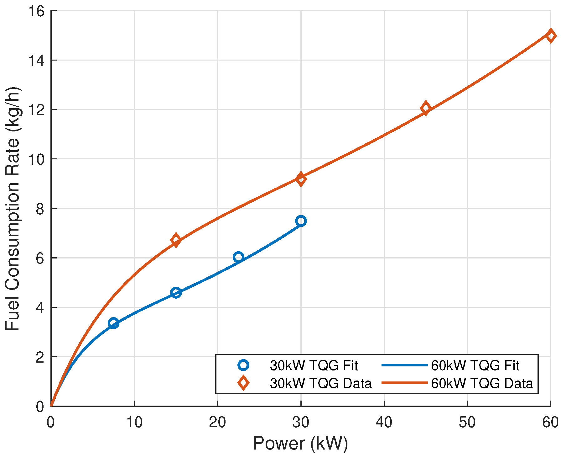
2.1. Generator Model

The EMS exploits load-dependent, diesel generator efficiency to reduce fuel consumption and energy storage requirements. Thus, this behavior must be captured in the generator’s model where the total fuel mass burned, m, is
m ( t ) = 0 t m ˙ ( P g , α g ) d τ
where P g is the generator’s time-varying power output, α g is a vector of generator-specific parameters, and m ˙ ( P g , α g ) is the generator’s load-dependent steady-state mass flow rate, often characterized by a generator’s flow rate versus power curve. In general the α g can be time-varying if aging effects are of interest. In the subsequent example, the microgrid contains four Tactical Quiet Generators (TQGs) [29]: two rated at 30 kW and two rated at 60 kW [30]. Their flow rate versus power characteristics are modeled as shown in Equation (2):
m ˙ ( P g , α g ) = α g , 1 e α g , 2 P g + α g , 3 e α g , 4 P g
where the elements of α g were determined to minimize the error between Equation (2) and the generator’s flow rate versus power data using nonlinear least squares and are shown in Table 1 with their corresponding plots in Figure 1. The exponential form of Equation (2) was used so that concatenating all the generators into a single fuel consumption curve yielded a continuous function. This was important for the optimization process used by the EMS as described below.

2.2. Energy Storage Model

Energy storage is usually needed in a microgrid to make full use of renewable sources when there is more generation than load or vice versa. The energy storage model used in the EMS, shown in Equation (3), is similar in form to the generator,
E ˙ s = P s ( E s , α s , t )
where E s is its instantaneous energy state, α s is a set of device-specific parameters, and P s is the power exiting the device. The negative sign indicates that when P s > 0 the storage device is discharging to service loads. Dependence on E s is required for some devices whose ability to source or sink energy depends on its energy state.
Two storage devices are used: (1) at the microgrid’s main bus, P s , b u s , and (2) collocated with each PV array, P s , p v . All storage devices were assumed to have the model form of Equation (4):
E s ( t ) = E s ( 0 ) α s , 1 0 t P s ( τ ) d τ , P s ( t ) 0 α s , 2 0 t P s ( τ ) d τ , P s ( t ) < 0
where the parameters α s , 1 and α s , 2 are the efficiencies for discharging and charging, respectively. The values used in the example of Section 4 are α s , 1 = 1.2 and α s , 2 = 0.8 . The storage initial state, E s ( 0 ) was set to 50 % of the energy capacity of 20,000 A · h per each energy storage device (bus storage and PV storage). The individual energy storage units were sized this way to ensure that sufficient energy storage reserves were present and a linear storage model could be used.

2.3. Photovoltaic Array with Collocated Storage Model

A PV array model is needed by the EMS to convert meteorological forecasts of ambient temperature, T a ( t ) , and irradiance, G ( t ) , into output power, P p v ( t ) . To be consistent with the fidelity of the generator and energy storage models described above, a steady-state approach is used with the general form of Equation (5):
P p v = P p v ( G , T a , α p v )
where α p v is a set of panel-specific parameters. The model used in this paper is the approach of Vergura et al. [31] that allows model construction based on parameters typically found on PV manufacturer data sheets. The parameter values used are shown in Table 2 and can be arranged in any convenient order to create the α p v of Equation (5).
PV arrays are controlled using maximum power point tracking (MPPT), and coupled with energy storage controlled by the EMS similar to the diesel generators.

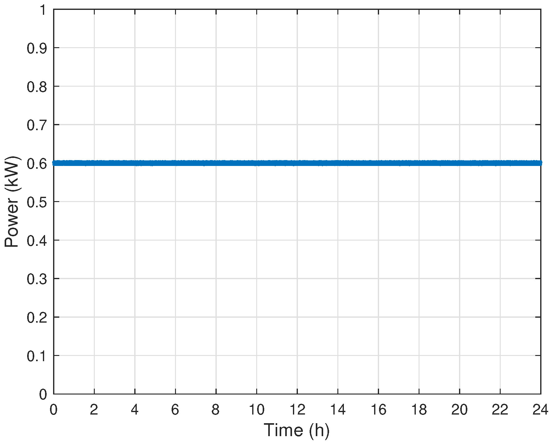
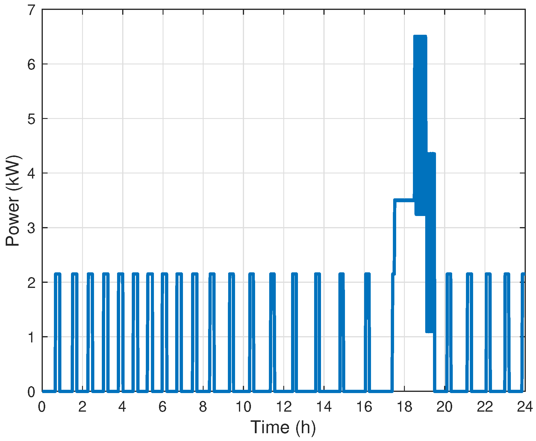
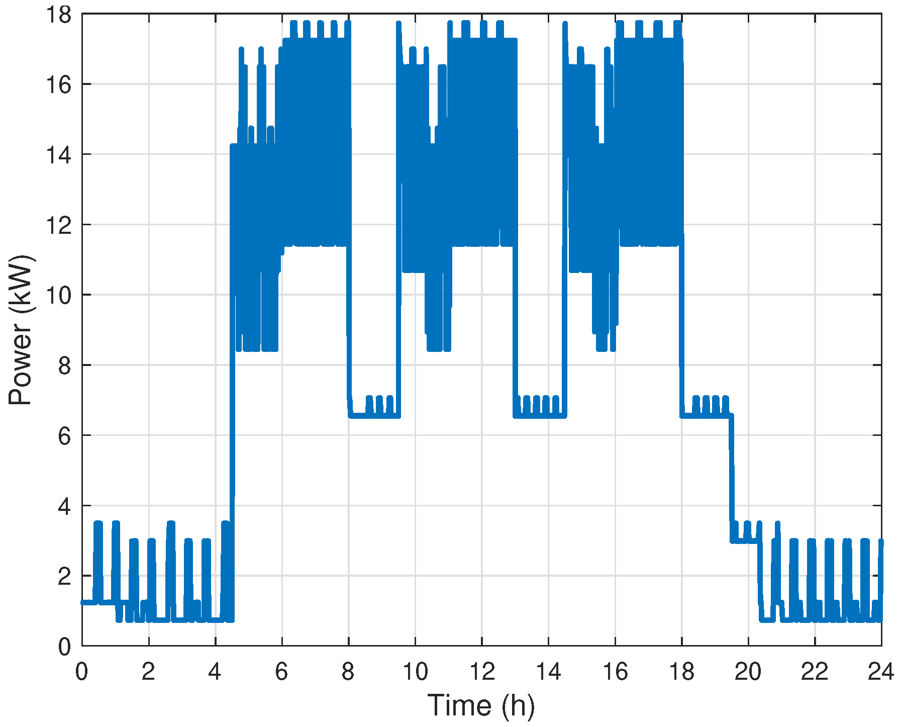
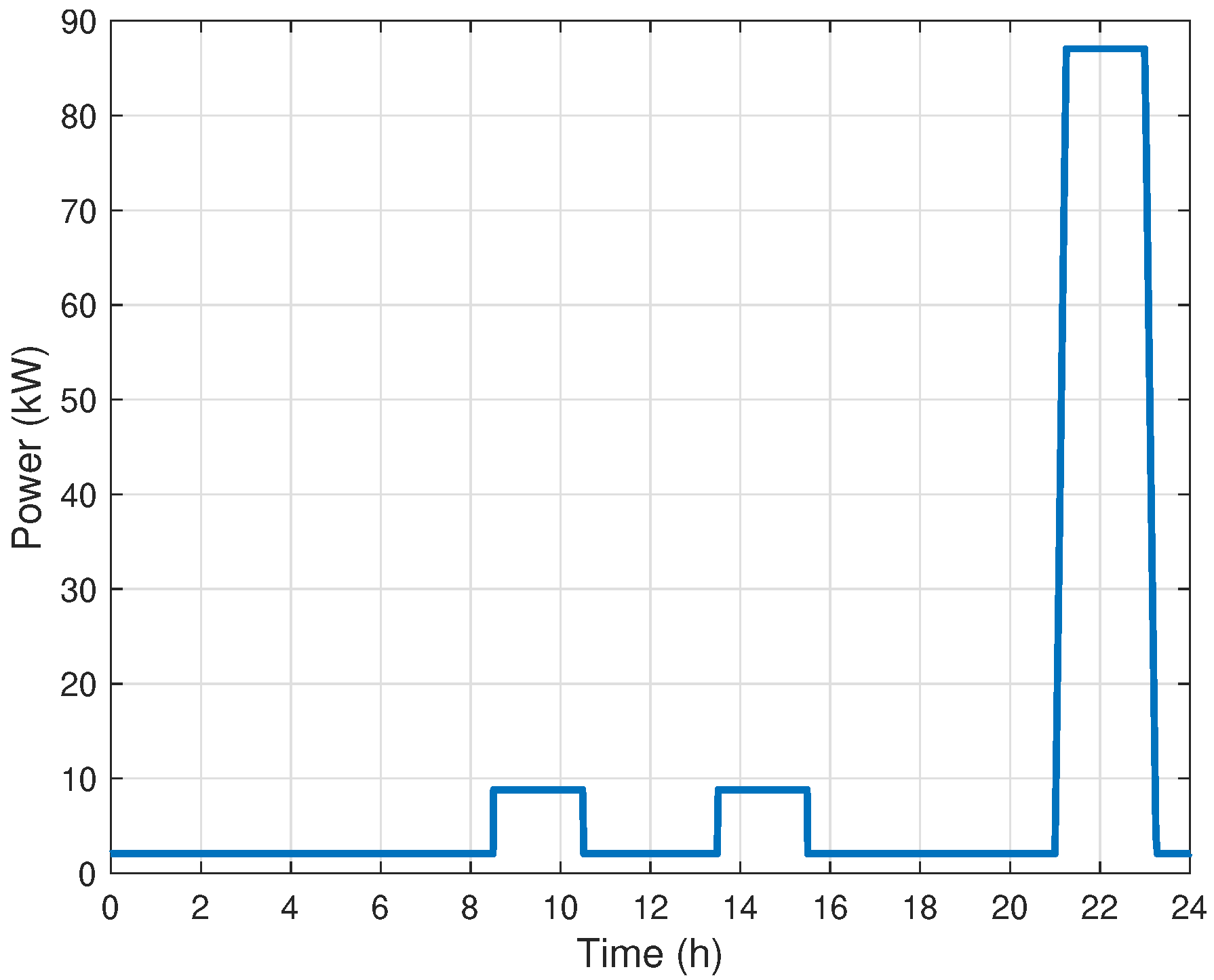
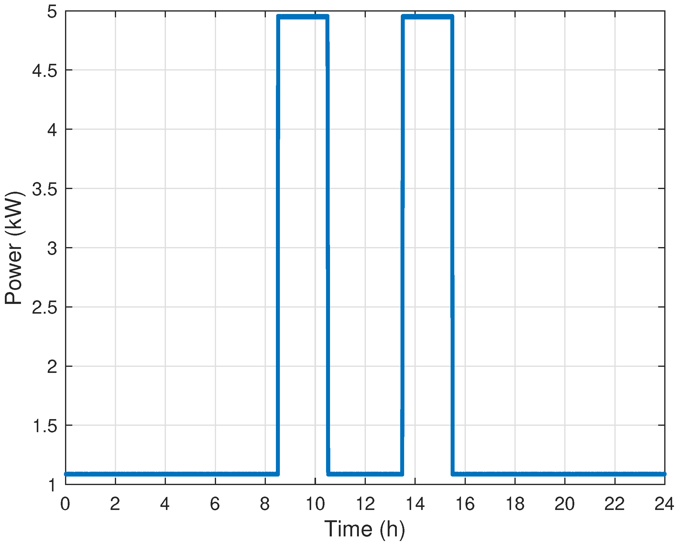
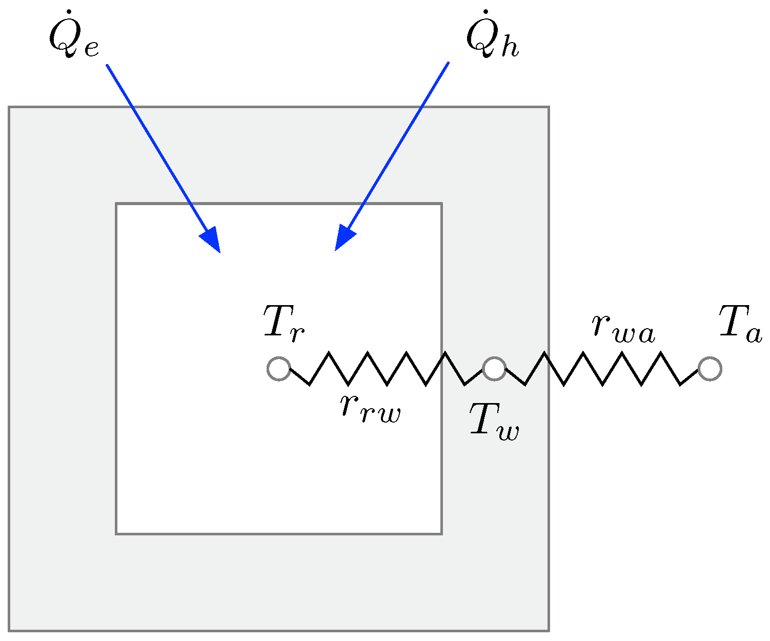
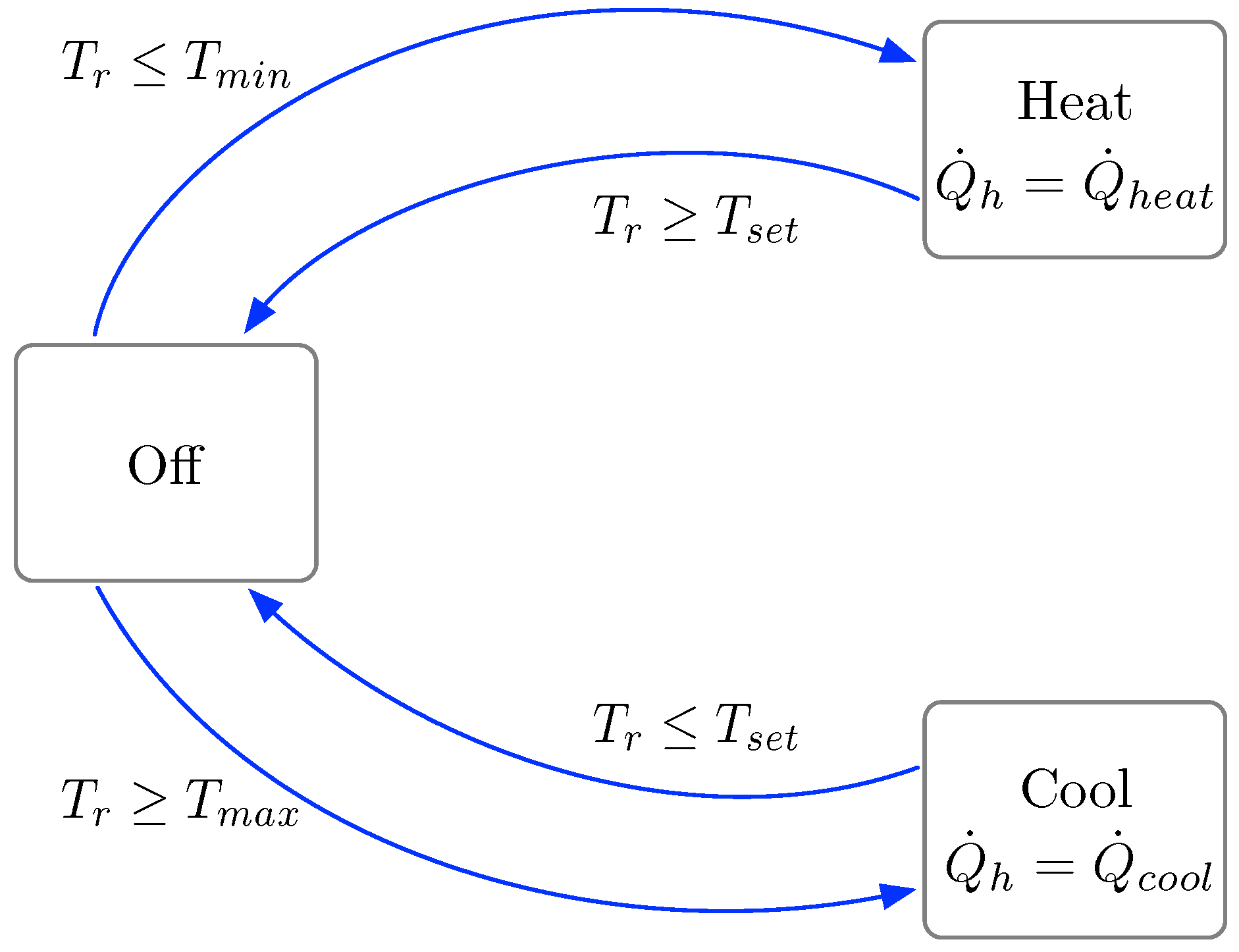
2.4. Electrical Load Model

The coupled, thermal, and electrical load model used by the EMS is shown in Equation (6), where T a is the ambient temperature; v is a binary valued, event trigger vector; P is made up of P l , b , the electrical load that is independent of T a ; and P l , T is that portion of the electrical load that depends on T a . Note that the EMS does not require that the total load be segregated into these two parts. However, since the focus of this work is to understand the effect of atmospheric conditions on fuel consumption and energy storage requirements, dividing the total load into these parts is helpful as will be seen in Section 4.
P l ( t ) = f ( v ( t ) , T a ( t ) )
The thermal and electrical loads were assumed to be coupled, due to shelters and their HVAC systems. The shelters’ thermal response is caused by both the ambient temperature and time-varying, event-driven internal thermal and electrical loads. For example, consider a mess hall with a meal event that defines both electrical loads (e.g., ovens, stoves water heating, etc.) and thermal loads (e.g., additional occupants, heat transfer from cooking equipment to the room, etc.) that are active for a known amount of time after the meal event begins. During this time the building’s total electrical load is the sum of the electrical loads of the meal event equipment and the HVAC system as it responds to heating due to the equipment and changes in T a .
The microgrid used in this study has eighteen shelters of seven different types. Each shelter type has a different equipment electrical load profile, P l , b , as described in Section 4.2.
Shelter thermal response is modeled using a lumped approach as shown in Figure 2. The air in the room has temperature T r and thermal capacitance C r , the wall has temperature T w with capacitance C w . The thermal resistance r r w includes the room’s air and wall, whereas r w a includes the wall and the outside air. The energy of the room’s air increases, Q ˙ e , due to events that define, for example, the number of occupants and the equipment being used. The closed-loop HVAC system also adds or removes energy, denoted Q ˙ h .
Applying conservation of energy to the control volume of Figure 2 generates two, first-order, linear differential equations for the building shown in Equation (7).
C r T ˙ r = 1 r r w T w T r + Q ˙ h + Q ˙ e C w T ˙ w = 1 r r w T w T r + 1 r w a T a T w
Thermal and electrical coupling arises from the event-driven heat input, Q ˙ e , and the electrically powered HVAC system. Thus, it is important that the HVAC system’s closed loop controller be approximated in the EMS.
The HVAC system uses an on–off control strategy with hysteresis shown in the state transition diagram of Figure 3. The room’s set point temperature, T s e t , and both the upper and lower bounds, T m i n and T m a x , are in general functions of v . Note that the controller parameters, T s e t , T m i n and T m a x could be included in an EMS strategy to exploit building thermal mass as energy storage, though that approach was not used in this analysis. The shelters’ HVAC parameters are T s e t = 63 C with T m i n = 58 C and T m a x = 68 C.
The electrical load due to the HVAC system, P h , is modeled using Equation (8), where COP h e a t and COP c o o l are the HVAC’s coefficients of performance for heating and cooling. The values used in the case study are Q ˙ h e a t = 10 kW, Q ˙ c o o l = 18 kW, COP h e a t = 1.8 and COP c o o l = 1.5 .
P h = Q ˙ h COP h e a t , heating Q ˙ h COP c o o l , cooling

3. Energy Management System

The EMS uses an MPC approach to update generator, P g , and PV storage power, P s , p v , commands every t u seconds to minimize the fuel consumed by the generators. It requires the models of Section 2 and estimates of both the load, P ^ l = P ^ l , b + P ^ l , T , and the PV output, P ^ p v , generated from meteorological forecasts of T ^ a and G ^ available every t p seconds where quantities with hats denote forecasts or estimates. At the start of the i t h control update cycle, t i , a discrete time, fuel-optimal solution, is computed out to the final time, t f . The constant, optimal values of P g ( t i ) and P s , p v ( t i ) are then issued to the generators and the PV storage for the next t u seconds. For the example of Section 4, t u = 900 s (15 min) and the meteorological forecast interval, t p , was varied from 15 min to 24 h.
For the case of n generators and m PV storage devices, the EMS must solve for t h t u ( n + m ) values within t u seconds. In the applications of interest, generators are more common than PV storage devices. Thus, steps were taken to make the EMS solution time invariant to the number of generators. This was achieved by using a single generator performance curve, as shown in Figure 1, by concatenating the performance curves of all the generators. If, for example, the EMS finds that the total optimal generator output should be 100 kW, then the two 30 kW generators would be run at full load and the 60 kW generator at partial load. Note that the order of concatenation constrains the solution space; however, this constraint can be removed by considering all unique concatenation types during the optimization process.
As the EMS used forecasted PV output and load values, in general, there was always a power imbalance. The bus storage, P s , b u s , was used as a slack asset to match the loads to generation. To reduce the effect of model errors, measurements of the actual storage and fuel consumed were used to update the model states prior to generating each new optimal solution.
The optimal control problem used by the MPC is defined as follows. Given the forecasts, T ^ a and G ^ and the models of Section 4, find the optimal total generator and the m PV storage commands, P g * , P s , p v , 1 * , P s , p v , m * , at each time step that minimizes the cost of Equation (9),
J = t i t f m ˙ ( P g , α g ) d τ
subject to the energy balance constraint of Equation (10),
j = 1 m E s , b u s , j ( t f ) + E s , p v , j ( t f ) = j = 1 m E s , b u s , j ( t o ) + E s , p v , j ( t o )
where P s , b u s and P p v , b u s were computed to ensure all the loads were met using Equation (12) and Equation (11):
P s , p v = j = 1 m P p v , b u s , j + P p v , j
P s , b u s = ( P l , b + P l , T ) P s , p v P g
and E s , b u s , j and E s , p v , j of Equation (10) are found by integrating Equation (12) and Equation (11), respectively.
The energy storage devices play an important role within the EMS, specifically required to account for the forecasting errors. First, the output of the PV was maximized using an MPPT. The resulting output was subtracted from the optimal PV commands issued by the EMS, then used to discharge or charge the PV’s collocated electrical storage. Second, the aggregation of all electrical loads were computed and subtracted from the aggregation of the optimal diesel generators and PV commands. Third, the subtraction operation results yielded the required bus storage’s electrical power contribution, making the bus storage the slack asset. Greater forecasting errors lead to more frequent charging/discharging of the storage assets, increasing the microgrid’s energy storage design requirements.
A network diagram (Figure 4) was provided to illustrate the relationships between the PV asset, diesel generator, electrical load, and the EMS. As shown in the figure, the EMS utilize weather forecasts constructed from the variable meteorological conditions. The weather forecast were converted into power forecasts using forecasters, which utilize the same electrical load and photovoltaic array models described previously. The power forecasts were then used in conjunction with updated microgrid measurements within our MPC’s optimization routines, which seeks to minimize fuel consumption while managing the distributed energy storage. The output of the MPC’s optimization was then used to control the individual microgrid asset, which respond to updated meteorological conditions. All states and signals displayed in the microgrid were then used to assess the performance of the microgrid and EMS subject to the variable weather conditions and PFs.

4. Meteorological Forecast Study

To illustrate the EMS and how its performance was affected by (1) the forecast interval, t u , and (2) the sky conditions, consider this example: The forecast interval is varied from 15 min to 24 h. The EMS computes a generator and PV storage solution using updated fuel consumption and energy storage states collected every 15 min. Four sky conditions are considered using measured solar radiation and temperature which give rise to four distinct electrical loads.
The context of the selected microgrid architecture was defined as a temporary ad hoc microgrid, constructed in response to a time-sensitive operation, located within a remote region, similar to a combat outpost (COP) or a disaster relief operation. Because of the high-tempo operation and isolated locality, it was presumed minimal past and present historical trends.
Because of the high-tempo operation and isolated locality, it was presumed minimal past and present historical trends. Thus a PWF was selected to estimate future atmospheric conditions from our scenario’s limited data resources. The atmospheric data selected for this example were extracted from the 2016 Base Camp Integration Laboratory (BCIL) demonstration.

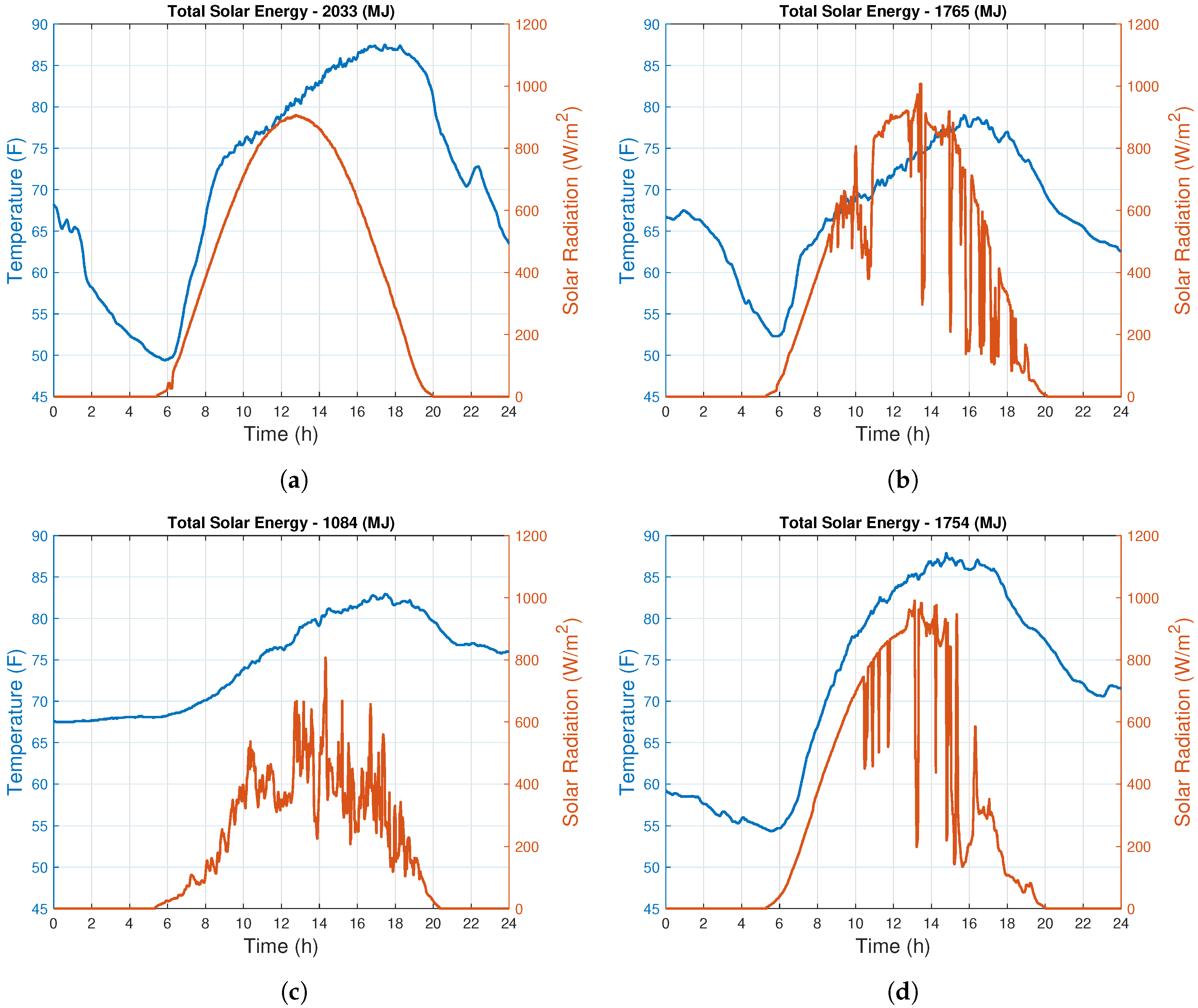
4.1. Meteorological Conditions

The EMS was evaluated over a 24 h epoch using temperature and solar radiation measurements for four representative sky conditions: clear (CLR), partly cloudy (PC), overcast (OVC), and monsoon (MON). The selected sky conditions were classified using the solar radiation profiles. These four sky conditions were gleaned from multiple atmospheric field studies conducted at the Army Research Laboratory (ARL), and represent four major scenarios from which the sky conditions have a significant impact on solar power generation.
As a simulation study, it was more important that the optimization routines were challenged with climatologically-representative samples of meteorological conditions, than provide “live” data from a weather service. The meteorological data sets were collected at 1 min averages, shown in Figure 5. The clear sky is characterized by its consistently smooth, Gaussian solar radiation curve. Partly cloudy conditions have a Gaussian-like solar radiation profile with intermittent dips caused by isolated cloud events. Overcast conditions have a solar radiation profile that has a Gaussian shape, with a significantly reduced amplitude with respect to clear or partly cloudy days. Like the partly cloudy case, intermittent dips are present due to the variation of cloud density within the overcast ceiling. The monsoon sky’s solar radiation time series includes all three previously described scenarios. The day begins similarly to the clear sky day. As midday approaches, the solar radiation becomes that of a partly cloudy day. By late afternoon it takes on the characteristics of the solar radiation time series equate to an overcast sky.
The temperature time series have unique, though less distinguished, attributes. For example, the clear sky case shows a strong cooling overnight, followed by a consistent temperature rise that persists until sunset, before waning in magnitude due to overnight clear sky radiative cooling. The partly cloudy case follows a similar pattern, except that the lowest and highest temperatures are more conservative. The overcast temperature time series begins with almost flat line values from mid-night to sunrise. Although the temperature does rise during the daylight hours, the magnitude of this rise is about one-third that of the clear sky case. After sundown, there is a cooling trend, but again, the magnitude is significantly less than the clear sky case. In the Monsoon temperature time series, the pre-dawn period shows a modest cooling, followed by a post-dawn, sharp temperature increase (coincident with the clear sky morning). Because of the increased cloud cover, the heat gained moderates through the subsequent hours. Radiative cooling under the overcast portion of the monsoon sky limits the extent of the expected cooling trend after sundown.

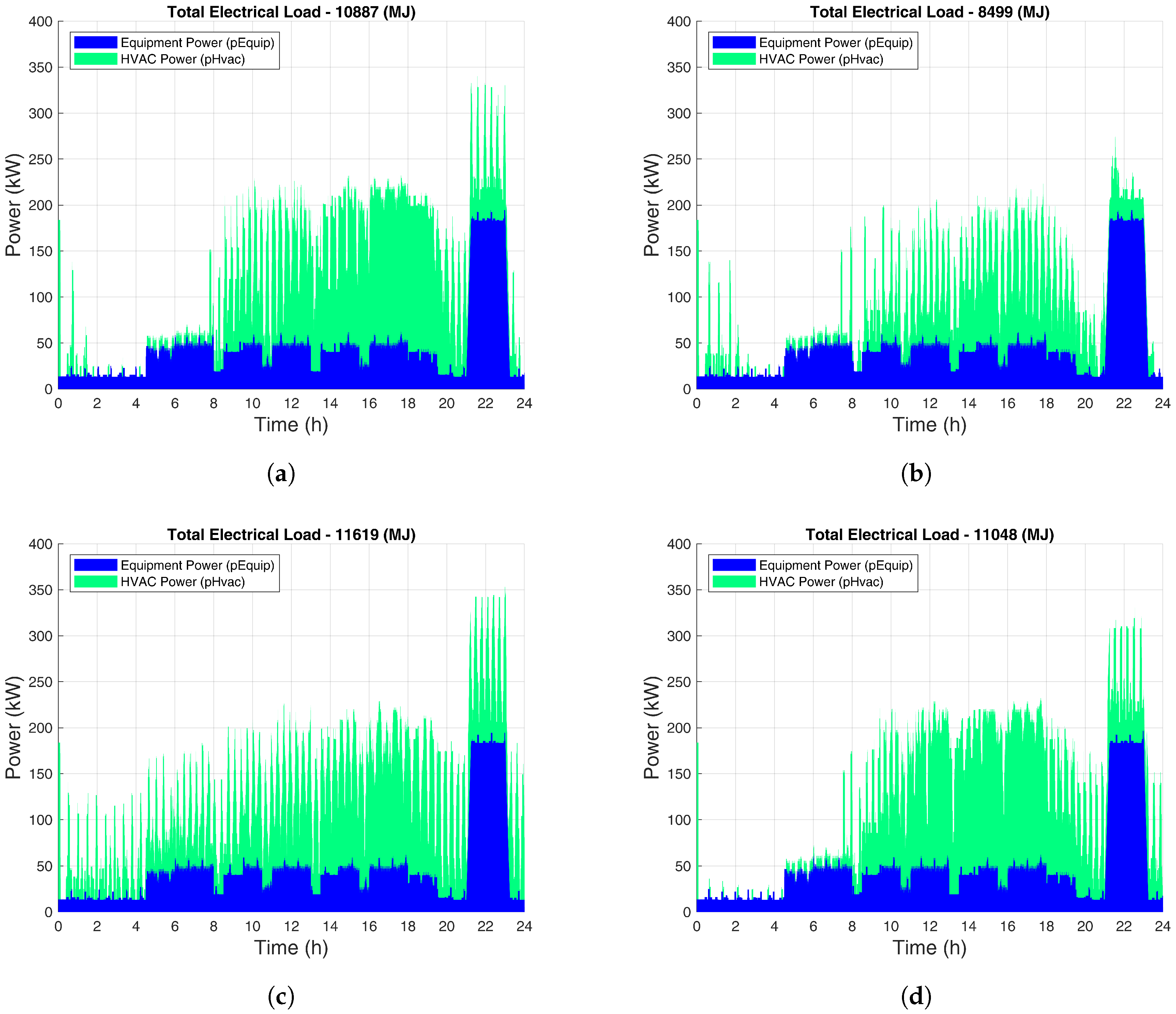
4.2. Microgrid and Electrical Load

The four-bus microgrid used in this example includes two 30 kW and two 60 kW diesel generators, bus storage, four 20 kW PV arrays each with PV storage, and eighteen shelters whose thermal constants with varying thermal constants. The grid’s time-varying electrical loads arise solely from shelter events, creating P l , b and temperature variations, leading to HVAC-induced P l , T profiles. The grid model, used to assess EMS performance, was simulated in MATLAB Simulink with an integration time step of 0.5 s. The EMS uses a similar model where persistence forecasted G ^ and T ^ a , and updates of storage and fuel states from the grid model, are used to estimate the future electrical load to solve for optimal generator and PV storage commands every 15 min. These new commands are then pushed to the grid model and zero-order held until the next update.
The eighteen shelters are of seven different types: eight billeting; two latrine; two shower; one laundry; one kitchen; two office; and two command, control and communication (COC/M). Each shelter of a given type has its own event schedule resulting in a P l , b time history. The kitchen typically contributed the largest electrical load, the exception was the COC/M shelters having large power spikes between 21 and 23 h. Shelter weather-dependent loads, P l , h , are due to their HVAC systems. These loads are typically three to four times those of the event-driven loads.
The grid electrical load for all four sky conditions—clear, partly cloudy, overcast, and monsoon—are shown in Figure 6. The total event-driven load is shown in blue, and the total weather-induced load is shown in green. As the event-driven loads are independent of sky conditions, they are identical in all four figures.

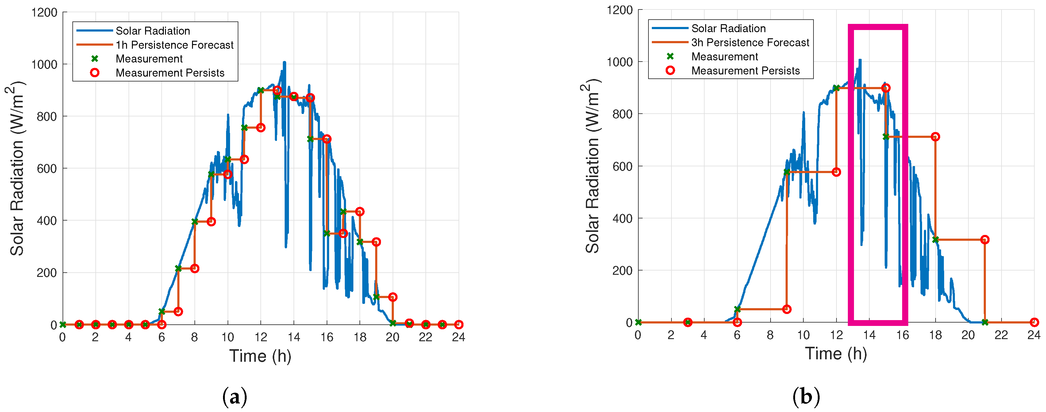
4.3. Persistence Weather Forecast (PWF)

The EMS uses a PWF, also called a “zero-order hold” forecast to estimate meteorological conditions. A PWF method was chosen over a Numerical Weather Prediction (NWP) model, based on the isolated gird scenario and its associated limitation. The effect of this forecasting method on the measured data is illustrated in Figure 7, using 1 and 3 h forecast intervals, respectively. If the PWF output occurs at a time of a sudden drop in solar radiation, the forecast incurs a significant error. In Figure 7a, this occurs between 1600 and 1700 h. Errors can also occur if the atmospheric conditions have frequent disruptions spanning a forecast interval. This behavior is also observed in Figure 7b as indicated by the box centered around the 15th hour mark. During this time interval, intermittent cloud cover reduces the solar irradiance that is not captured by the forecast.
A PWF assumes that the current conditions persist for some forecast interval or horizon, where the forecast interval dictates the discretization of the forecast horizon. In the case of this study, variable forecast intervals were used with a set forecast horizon of 24 h. It was assumed that midnight marked the beginning and end of the forecast horizon encapsulating a 24 h period. When constructing a 3 h PWF, the value of the solar radiation at midnight was observed, this value then persists for the next three hours. Three hours from midnight, the next value of solar radiation was observed; similarly, the value persists for the following three hours. This process is completed until the PWF was constructed (Figure 7b). Using the predefined meteorological weather scenarios, the PWFs can be constructed using variable forecast intervals. The variable forecast intervals introduce uncertainty and have the potential to degrade the power forecast, potentially degrading the performance of the microgrid and EMS.

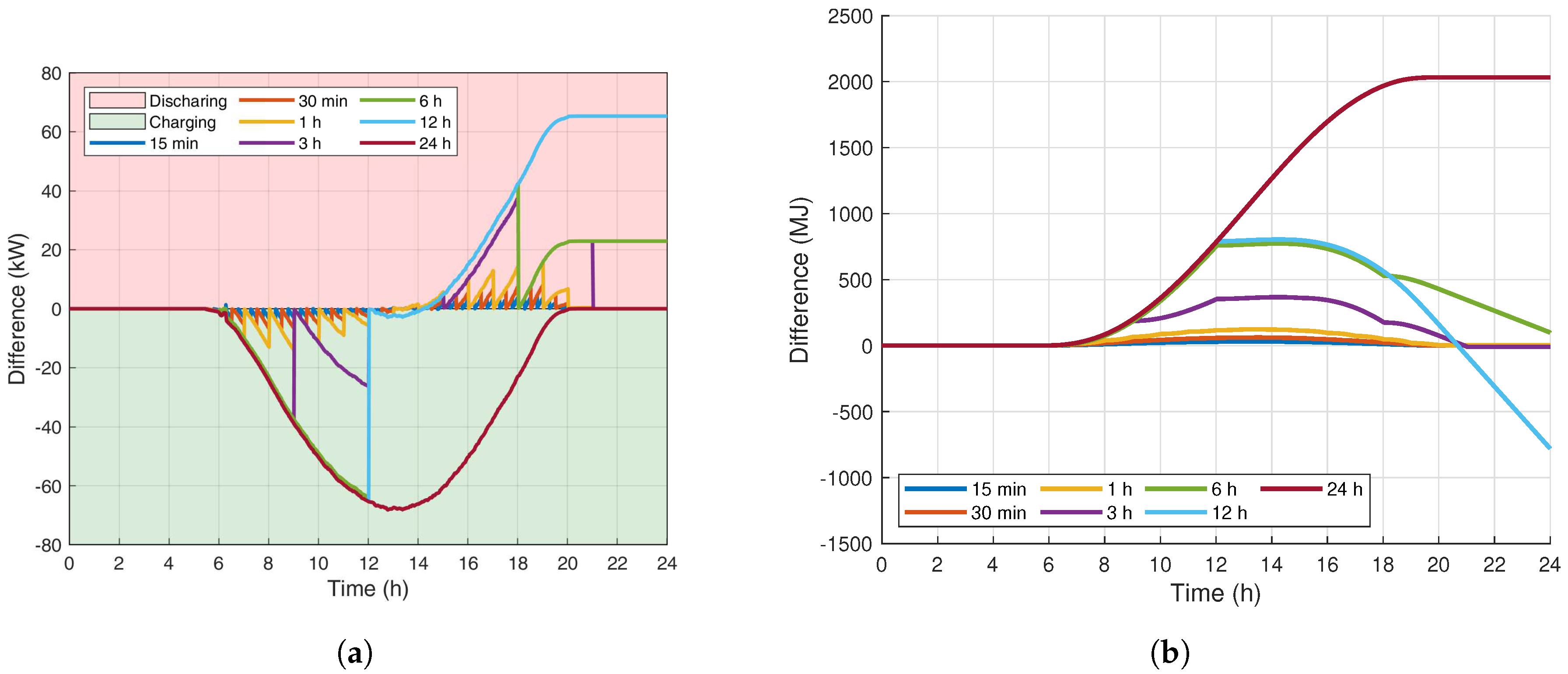
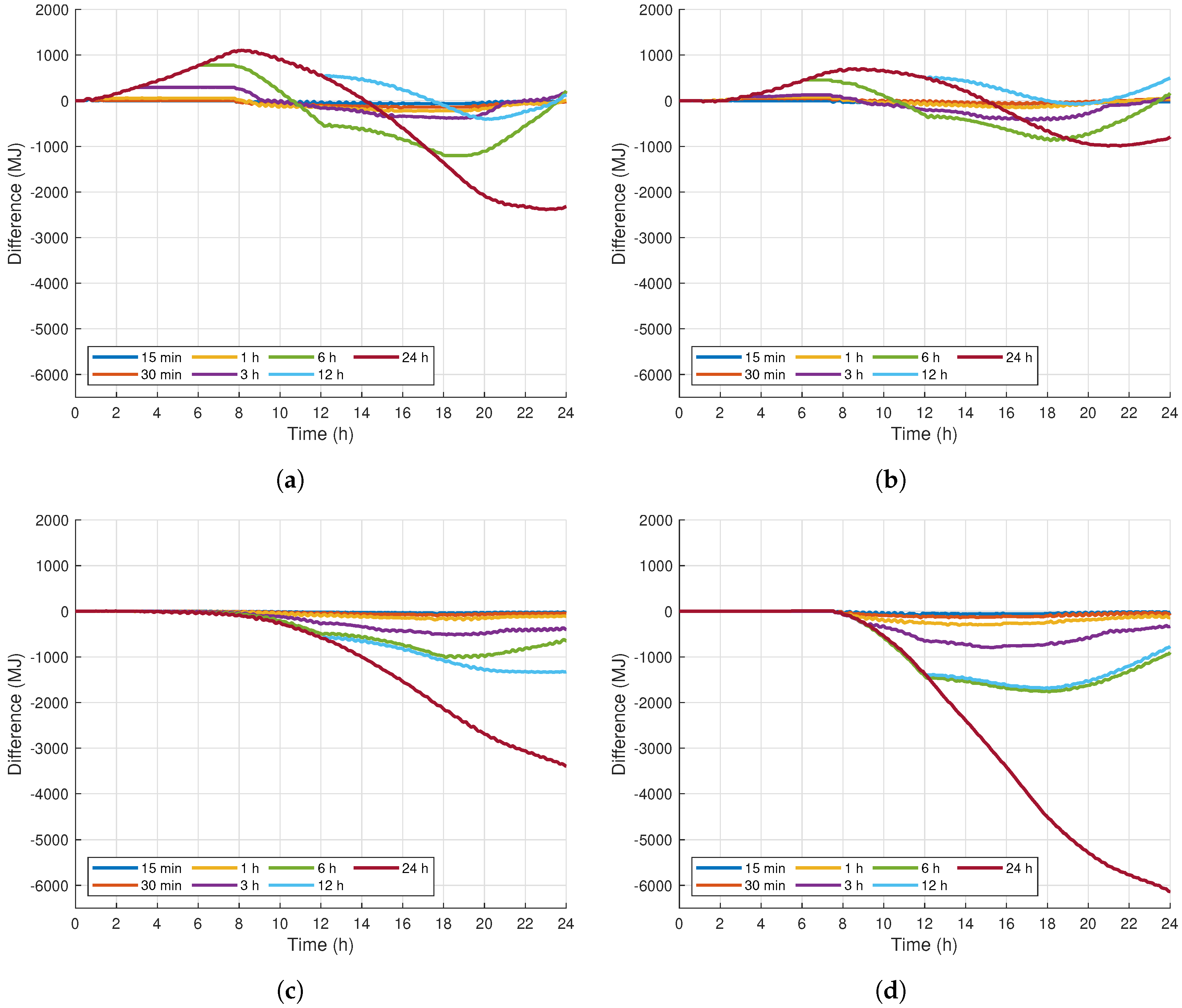
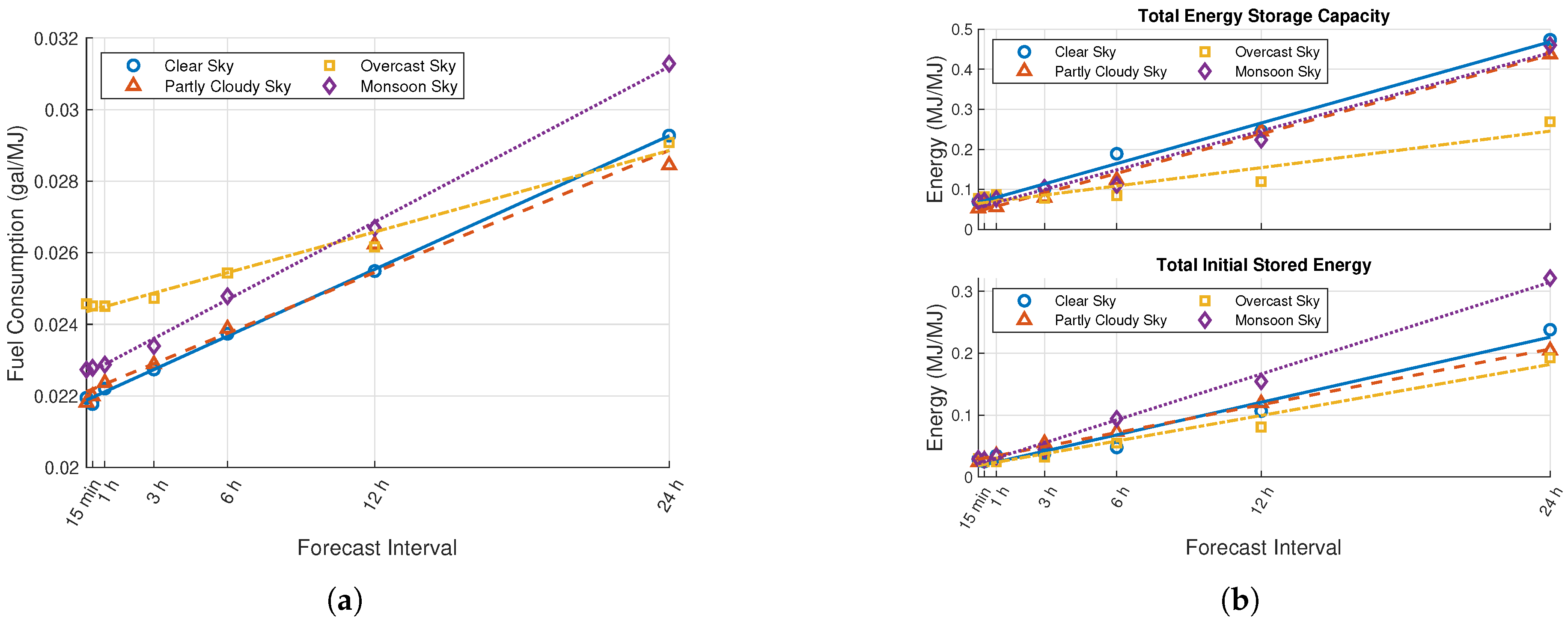
4.4. Results and Discussion

The effect of weather/load forecast intervals and sky conditions on the EMS performance was evaluated using the microgrid model with t u ranging from 15 min to 24 h. Forecast intervals less than 15 min were not considered, as 15 min was the update period of the EMS.
The clear sky PV power and energy forecast differences are provided in Figure 8. For completeness, the other atmospheric sky condition results are provided in the Appendix A. The power forecast difference is computed as P d i f ( t ) = P ^ s , p v ( t ) P s , p v ( t ) , the resulting energy difference is then E d i f = 0 P d i f ( t ) d τ ; these equations arise as negative power is consistent with charging, whereas positive power is consistent with discharging.
As a result of the PWF shown in Figure 7, the differences between the forecasted and actual PV power production drive the storage actuation in the EMS. This leads to underestimation of PV power production prior to solar noon, charging the PV’s collocated electrical storage (negative differences in Figure 8a). Conversely, overestimation of the PV power production occurs after solar noon, discharging the energy storage (Positive differences in Figure 8b). As the forecast interval increases, the magnitude of the PV power forecast differences increases, growing the energy forecast differences. Larger energy forecast differences generally lead to larger energy storage design requirements. The PV power and energy forecast differences are dependent on the variable sky conditions. For example, the overcast sky conditions were the smallest, while the clear sky conditions were the largest.
The forecast differences were then quantified for the time-varying temperature dependent electrical load, provided in Figure 9. Power forecast differences were integrated to form the energy forecast differences.
The power forecast difference is computed as P d i f ( t ) = P ^ l ( t ) P l ( t ) , the resulting energy difference is then E d i f = 0 P d i f ( t ) d τ , these equations arise as negative power is consistent with charging, whereas positive power is consistent with discharging. Similarly to the PV’s energy forecast differences, smaller forecast intervals seemingly require less actuation of the bus storage, minimizing the energy storage design requirements for the microgrid. Conversely, as the forecast intervals increase, greater amounts of energy storage are required for each of the four atmospheric sky conditions. Similarly, the load energy forecast differences are dependent on the variable sky conditions.
The EMS’s optimization algorithm issues the optimal PV and diesel generator commands that minimize fuel consumption and energy storage requirements for the microgrid. The commands issued by the EMS dictate the exact amount of energy charged or discharged by either the PV’s collocated energy storage or the bus storage. Thus, Figure 8 and Figure 9 represent the absolute worse case in which the forecasting differences are entirely accounted for by the energy storage, without the use of the diesel generators.
Microgrid performance was then measured using three metrics: generator fuel consumption, energy storage capacity, and initial energy storage state. These three metrics are shown in Figure 10, along with least square error line fits. The microgrid performance metrics were normalized by dividing their raw values by the total energy consumed by the microgrid loads over the 24 h epoch. These values were shown for the clear, partly cloudy, monsoon and overcast days in Figure 6 and are 10,887 MJ, 8499 MJ, 11,619 MJ, and 11,048 MJ, respectively. The normalizing method allows for a better comparison between the four types of sky conditions. It also enables the results to be extended to other load scenarios.
The t u = 15 min point, shown in all three metric plots, is the best case situation where the forecast and EMS updates are equal minimizing the errors between forecasted and true loads, as well as meteorological conditions. The slopes of the lines indicate the sensitivity of the metrics to t u . In all cases, the metrics increased linearly with increased forecast intervals. This sensitivity to t u can be explained by changes in both the loads and the meteorological conditions that were not forecasted yet occurred between EMS updates.
The normalized fuel consumption of Figure 10a is greatest for the overcast day compared to the other sky condition cases at t u = 15 min. This attribute can be explained by the overcast conditions producing the least amount of PV energy. However, forecast interval sensitivity during overcast conditions is four times less than the monsoon day, which has the greatest sensitivity to t u . The clear and partly cloudy cases have nearly identical forecast update sensitivities. These results point to a dependence of the normalized fuel consumption on the daily variation in the meteorological conditions.
The storage results are shown in Figure 10b, where for t u = 15 min. Both the normalized storage capacity and the normalized initial storage state are invariant with respect to sky condition. The normalized units are MJ Storage per MJ Daily Electrical Load. Thus, to calculate the required storage, the values in the plots should be multiplied by the expected daily load.
Like the normalized fuel consumption, both storage metrics show the least t u sensitivity on the overcast day. The normalized initial storage energy on the monsoon day has a significant t u sensitivity compared to the other sky cases. This relationship is likely due to the numerous unforecasted drops in PV generation that require unplanned bus storage to balance the grid.

5. Conclusions and Future Work

The use of the PWF method consistently led to under predictions within the PV’s power forecasts prior to solar noon. As a result of this behavior, the PV’s collocated electrical storage tends to more regularly charge. After solar noon, the same predictions then overestimate, leading to discharging of the PV’s collocated electrical storage. The observed trend means the PV is less likely to have an impact on the overall initial energy storage design metric for a microgrid, as the energy storage will begin building up a reserve of energy prior to atmospheric disturbances, which is perhaps more desirable.
The length of a weather forecast interval was shown to affect both the daily EMS performance, in terms of fuel consumption, and the microgrid design, in terms of the required storage capacity. To ensure peak generator efficiency, the EMS relied on the temperature forecast to predict both load types and the PV generation. Longer forecast intervals resulted in load and PV generation errors, leading to two undesirable outcomes. First, the EMS was forced to rely more heavily on the bus storage to balance the grid; and thus the grid design required more energy storage. Operating with the least amount of storage was desirable from a cost, maintenance, and weight perspective. Second, the amount of time the generators were operated outside their peak efficiency increased as t u increased, resulting in increased fuel consumption.
The case study above was meant to illustrate the EMS and how its performance was affected by meteorological conditions for a limited set of cases and a particular microgrid architecture. The approach, however, can also be used for other microgrid designs, if a wider set of conditions is explored for both event-based loads and meteorological conditions.
The PWF used here was intended as a baseline technique. Future work includes using more accurate temperature and solar radiation forecasting strategies, as well as, the exploitation of shortened forecast intervals.
The studies were completed in an attempt to characterize the meteorological forecast impact on microgrid optimization performance and design, subject to variable forecast interval, and variable sky conditions for an extended duration. The approach included developing the EMS.
As this was the first instantiation of the EMS, simplified models were used within this study that could easily be verified and altered to permit ease in identifying and assessing the microgrid performance subject to the variable atmospheric conditions and forecasts. Future work would include deploying the EMS on higher fidelity models.

Author Contributions

The individual contributions of each of the four authors R.J., G.P., G.V., and M.B. are as follows; Conceptualization, R.J. and G.P.; Data curation, R.J. and G.P.; Formal analysis, R.J. and G.P.; Funding acquisition, M.B.; Investigation, R.J. and G.P.; Methodology, R.J. and G.P.; Project administration, M.B.; Resources, G.V. and M.B.; Software, R.J. and G.P.; Supervision, G.P.; Validation, R.J. and G.P.; Visualization, R.J., G.P., G.V., and M.B.; Writing—original draft, R.J. and G.P.; Writing—review & editing, R.J., G.P., G.V., and M.B. All authors have read and agreed to the published version of the manuscript.

Funding

This work was supported by the U.S. Army Futures Command Army Research Laboratory (ARL) under the contract CA W911NF-17-2-0130.

Acknowledgments

The authors would like to thank Michael Cook of the Milwaukee School of Engineering (MSOE) for his contribution that lead to the development of the event scheduler used to create the equipment loads.

Conflicts of Interest

The authors declare no conflicts of interest.

Disclaimer

Reference herein to any specific commercial company, product, process, or service by trade name, trademark, manufacturer, or otherwise, does not necessarily constitute or imply its endorsement, recommendation, or favoring by the United States Government or the Department of the Army (DoA). The opinions of the authors expressed herein do not necessarily state or reflect those of the United State Government of the DoA, and shall not be used for advertising or product endorsement purposes; Components of this publication were also used to fulfill the degree requirements for pursuit of a doctoral degree, in the field of Mechanical Engineering—Engineering Mechanics at Michigan Technological University [32]; DISTRIBUTION STATEMENT A. Approved for public release: distribution unlimited.

Appendix A

This appendix contains additional parameters, constants, and results which were not included within the main publication. Appendix A.1 includes additional results for the partly cloudy sky results, and Appendix A.3 includes additional results for the monsoon sky results. Appendix A.4 contains information regarding the thermal constants and parameters which define the thermal behavior of the HVAC, in addition to the event driven electrical load which was held constant and required by the MPC to estimate the aggregate electrical load.

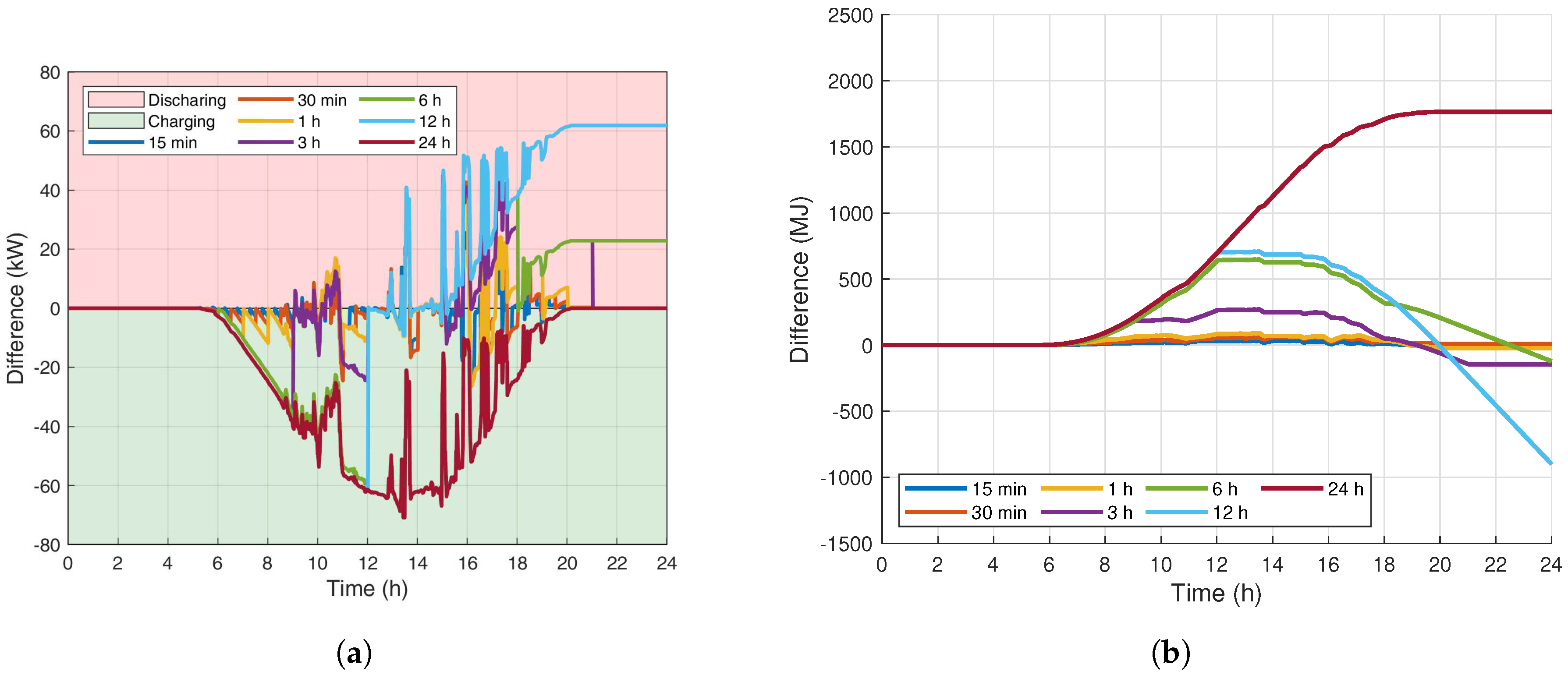
Appendix A.1. Partly Cloudy Sky Results

Figure A1. The resulting PV power and energy forecast differences that arise from the use of temperature and solar irradiance forecast when compared to the known truth atmospheric time series of the renewable asset assuming MPPT for the partly cloudy sky conditions. (a) The partly cloudy sky PV power forecast differences. (b) The partly cloudy sky PV energy forecast differences.
Energies 13 00577 g0a1

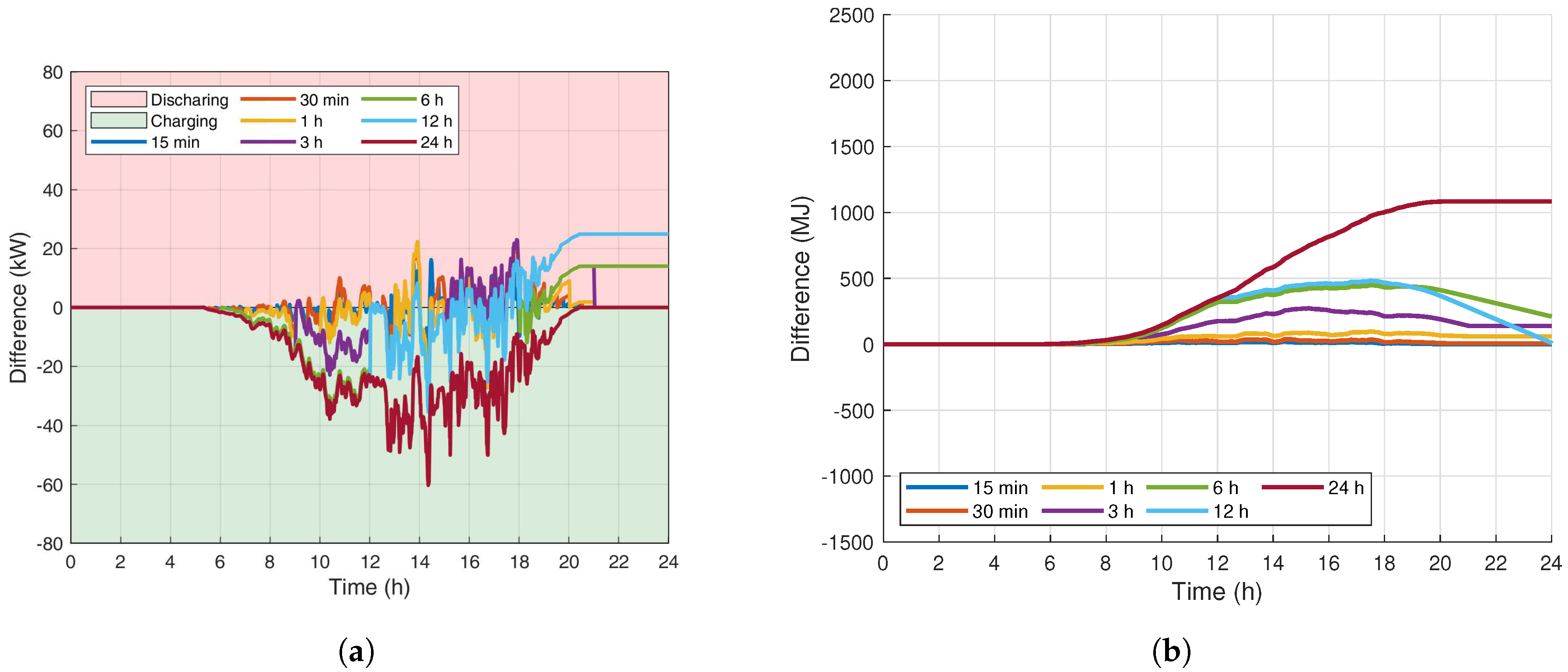
Appendix A.2. Overcast Sky Results

Figure A2. The resulting PV power and energy forecast differences that arise from the use of temperature and solar irradiance forecast when compared to the known truth atmospheric time series of the renewable asset assuming MPPT for the overcast sky conditions. (a) The overcast sky PV power forecast differences; (b) The overcast sky PV energy forecast differences.
Energies 13 00577 g0a2

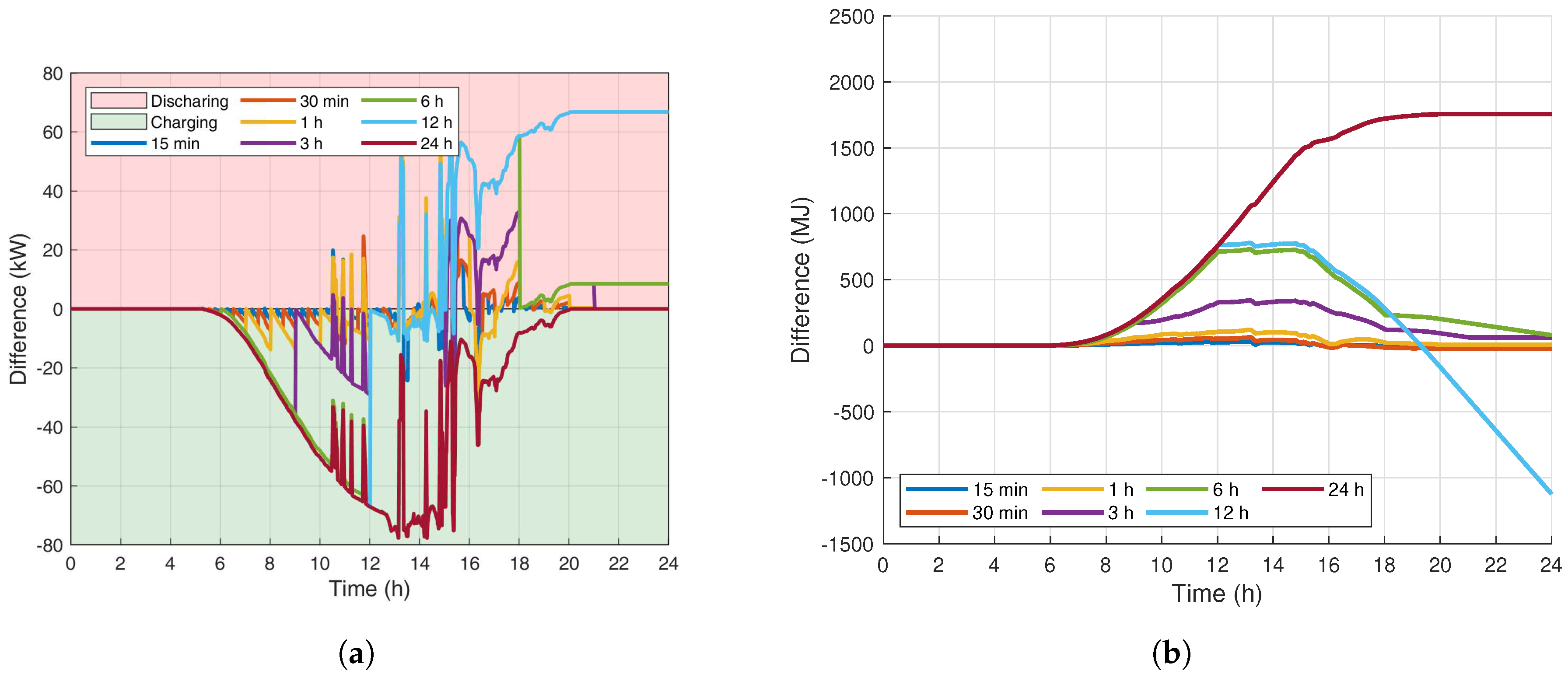
Appendix A.3. Monsoon Sky Results

Figure A3. The resulting PV power and energy forecast differences that arise from the use of temperature and solar irradiance forecast when compared to the known truth atmospheric time series of the renewable asset assuming MPPT for the monsoon sky conditions. (a) The monsoon sky PV power forecast differences. (b) The monsoon sky PV energy forecast differences.
Energies 13 00577 g0a3

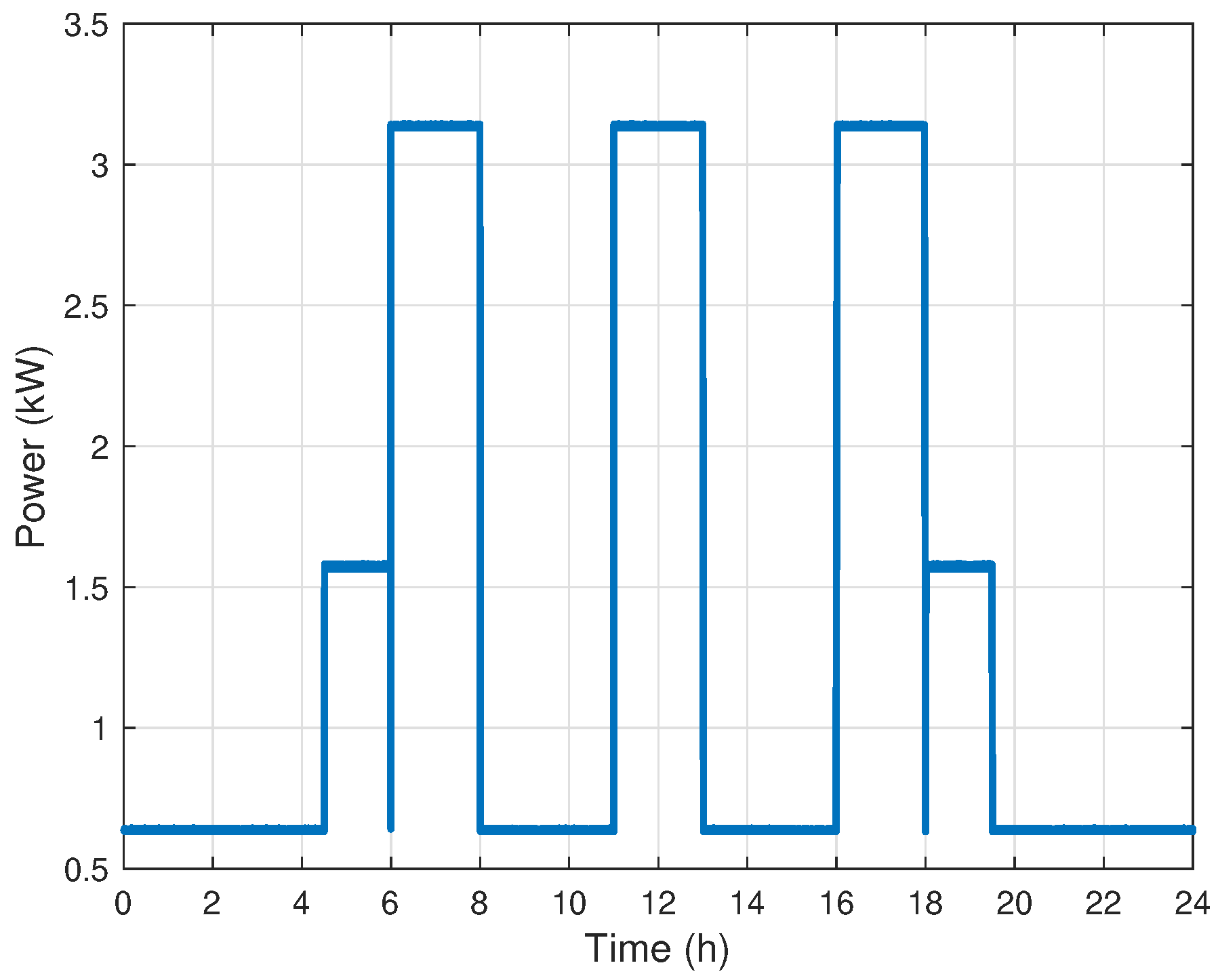
Appendix A.4. Electrical Load

Seven shelter types were used in the microgrid architecture: (1) billeting, (2) latrine, (3) laundry, (4) shower, (5) kitchen, (6) office, and (7) the combat operations center and communication (COC/M). Each shelter type had a unique internal equipment electrical load and are provided in Figure A4, Figure A5, Figure A6, Figure A7, Figure A8, Figure A9, Figure A10.
Figure A4. Billeting shelter equipment power.
Energies 13 00577 g0a4
Figure A5. Latrine shelter equipment power.
Energies 13 00577 g0a5
Figure A6. Laundry shelter equipment power.
Energies 13 00577 g0a6
Figure A7. Shower shelter equipment power.
Energies 13 00577 g0a7
Figure A8. Kitchen shelter equipment power.
Energies 13 00577 g0a8
Figure A9. COC/M shelter equipment power.
Energies 13 00577 g0a9
Figure A10. Office shelter equipment power.
Energies 13 00577 g0a10
The shelter model of Equation (7), used in the EMS, required several parameters. The room thermal capacitance, C r was calculated as shown in Equation (A1) with the physical parameters of Table A1.
C r = C p , a i r ρ a i r V r
Table A1. Thermal parameters common to all shelter.
SymbolDescriptionUnitValue
C p , a i r Average specific heat of air k J k g K 1 1.005
ρ a i r Density of air k g m 3 1.19
V r Room volume m 3 650.0
Shelter thermal resistances were computed using Equations (A2)–(A6) based on room and wall thermal time constants given in Table A2.
Table A2. Shelter-specific thermal parameters.
ShelterShelterWallWall TimeRoom Time
NumberTypeCapacitance, C w Constant, τ w Constant, τ r
kJ kg 1 ss
1Billeting232323
2Billeting303030
3Billeting292929
4Billeting252525
5Latrine262626
6Billeting303030
7Billeting232323
8Billeting303030
9Billeting282828
10Latrine212121
11Shower242424
12Shower303030
13Laundry292929
14Kitchen12147147
15COC212121
16COM262626
17Office202020
18Office272727
r r = C r / τ r
r w = C w / τ w
r a = r r
r r w = r r + 1 2 r w
r w a = r a + 1 2 r w

References

  1. Li, F.; Li, R.; Zhou, F. Microgrid Technology and Engineering Application; Elsevier: Amsterdam, The Netherlands, 2015. [Google Scholar]
  2. Brewster, K.; Degelia, S.; Mueller, D. Potential Availability and Stability of Solar Power in Oklahoma White Paper. 2014. Available online: https://studylib.net/doc/8691353/solar-white-paper (accessed on 5 August 2019).
  3. Blumsack, S.; Richardson, K. Cost and emissions implications of coupling wind and solar power. Smart Grid Renew. Energy 2012, 3, 308. [Google Scholar] [CrossRef] [Green Version]
  4. Inman, R.H.; Pedro, H.T.; Coimbra, C.F. Solar forecasting methods for renewable energy integration. Prog. Energy Combust. Sci. 2013, 39, 535–576. [Google Scholar] [CrossRef]
  5. Reikard, G. Predicting solar radiation at high resolutions: A comparison of time series forecasts. Solar Energy 2009, 83, 342–349. [Google Scholar] [CrossRef]
  6. Husein, M.; Chung, I.Y. Day-Ahead Solar Irradiance Forecasting for Microgrids Using a Long Short-Term Memory Recurrent Neural Network: A Deep Learning Approach. Energies 2019, 12, 1856. [Google Scholar] [CrossRef] [Green Version]
  7. Chow, C.W.; Urquhart, B.; Lave, M.; Dominguez, A.; Kleissl, J.; Shields, J.; Washom, B. Intra-hour forecasting with a total sky imager at the UC San Diego solar energy testbed. Solar Energy 2011, 85, 2881–2893. [Google Scholar] [CrossRef] [Green Version]
  8. Chow, C.W.; Belongie, S.; Kleissl, J. Cloud motion and stability estimation for intra-hour solar forecasting. Solar Energy 2015, 115, 645–655. [Google Scholar] [CrossRef]
  9. Abdel-Aal, R.E. Hourly temperature forecasting using abductive networks. Eng. Appl. Artif. Intell. 2004, 17, 543–556. [Google Scholar] [CrossRef]
  10. Dombaycı, Ö.A.; Gölcü, M. Daily means ambient temperature prediction using artificial neural network method: A case study of Turkey. Renew. Energy 2009, 34, 1158–1161. [Google Scholar] [CrossRef]
  11. Antonanzas, J.; Osorio, N.; Escobar, R.; Urraca, R.; Martinez-de-Pison, F.J.; Antonanzas-Torres, F. Review of photovoltaic power forecasting. Solar Energy 2016, 136, 78–111. [Google Scholar] [CrossRef]
  12. Shi, J.; Lee, W.J.; Liu, Y.; Yang, Y.; Wang, P. Forecasting power output of photovoltaic systems based on weather classification and support vector machines. IEEE Trans. Ind. Appl. 2012, 48, 1064–1069. [Google Scholar] [CrossRef]
  13. Tao, C.; Duan, S.; Chen, C. Forecasting power output for grid-connected photovoltaic power system without using solar radiation measurement. In Proceedings of the 2nd International Symposium on Power Electronics for Distributed Generation Systems, Hefei, China, 16–18 June 2010. [Google Scholar]
  14. Islahi, A.; Saani, S.; Mostafa, H. Hottel’s Clear Day Model for a typical arid city-Jeddah. Int. J. Eng. Sci. Invent. 2015, 4, 32–37. [Google Scholar]
  15. Yang, H.T.; Huang, C.M.; Huang, Y.C.; Pai, Y.S. A weather-based hybrid method for 1-day ahead hourly forecasting of PV power output. IEEE Trans. Sustain. Energy 2014, 5, 917–926. [Google Scholar] [CrossRef]
  16. Bouzerdoum, M.; Mellit, A.; Pava, N.A.M. A hybrid model (SARIMA–SVM) for short-term power forecasting of a small-scale grid-connected photovoltaic plant. Solar Energy 2013, 98, 226–235. [Google Scholar] [CrossRef]
  17. Sáez, D.; Ávila, F.; Olivares, D.; Cañizares, C.; Marín, L. Fuzzy prediction interval models for forecasting renewable resources and loads in microgrids. IEEE Trans. Smart Grid 2014, 6, 548–556. [Google Scholar] [CrossRef] [Green Version]
  18. Nespoli, A.; Mussetta, M.; Ogliari, E.; Leva, S.; Fernández-Ramírez, L.; García-Triviño, P. Robust 24 Hours ahead Forecast in a Microgrid: A Real Case Study. Electronics 2019, 8, 1434. [Google Scholar] [CrossRef] [Green Version]
  19. Sala, S.; Amendola, A.; Leva, S.; Mussetta, M.; Niccolai, A.; Ogliari, E. Comparison of Data-Driven Techniques for Nowcasting Applied to an Industrial-Scale Photovoltaic Plant. Energies 2019, 12, 4520. [Google Scholar] [CrossRef] [Green Version]
  20. Hong, T.; Wilson, J.; Xie, J. Long term probabilistic load forecasting and normalization with hourly information. IEEE Trans. Smart Grid 2013, 5, 456–462. [Google Scholar] [CrossRef]
  21. Hernandez, L.; Baladron, C.; Aguiar, J.M.; Carro, B.; Sanchez-Esguevillas, A.J.; Lloret, J.; Massana, J. A survey on electric power demand forecasting: Future trends in smart grids, microgrids and smart buildings. IEEE Commun. Surv. Tutor. 2014, 16, 1460–1495. [Google Scholar] [CrossRef]
  22. Yu, C.N.; Mirowski, P.; Ho, T.K. A sparse coding approach to household electricity demand forecasting in smart grids. IEEE Trans. Smart Grid 2016, 8, 738–748. [Google Scholar] [CrossRef]
  23. Zhou, H.; Bhattacharya, T.; Tran, D.; Siew, T.S.; Khambadkone, A.M. Composite energy storage system involving battery and ultracapacitor with dynamic energy management in microgrid applications. IEEE Trans. Power Electron. 2010, 26, 923–930. [Google Scholar] [CrossRef]
  24. Lu, D.; Francois, B. Strategic framework of an energy management of a microgrid with a photovoltaic-based active generator. In Proceedings of the 2009 8th International Symposium on Advanced Electromechanical Motion Systems & Electric Drives Joint Symposium, Lille, France, 1–3 July 2009. [Google Scholar]
  25. Moretti, L.; Polimeni, S.; Meraldi, L.; Raboni, P.; Leva, S.; Manzolini, G. Assessing the impact of a two-layer predictive dispatch algorithm on design and operation of off-grid hybrid microgrids. Renew. Energy 2019, 143, 1439–1453. [Google Scholar] [CrossRef]
  26. Shi, W.; Xie, X.; Chu, C.C.; Gadh, R. Distributed optimal energy management in microgrids. IEEE Trans. Smart Grid 2014, 6, 1137–1146. [Google Scholar] [CrossRef]
  27. Su, W.; Wang, J.; Roh, J. Stochastic energy scheduling in microgrids with intermittent renewable energy resources. IEEE Trans. Smart Grid 2013, 5, 1876–1883. [Google Scholar] [CrossRef]
  28. Hayes, B.P.; Prodanovic, M. State forecasting and operational planning for distribution network energy management systems. IEEE Trans. Smart Grid 2015, 7, 1002–1011. [Google Scholar] [CrossRef]
  29. GlobalSecurity.org. Tactical Quiet Generators. Available online: https://www.globalsecurity.org/military/systems/ground/mep-tqg.htm (accessed on 22 July 2019).
  30. Rizzo, D.M. US Army CCDC Ground Vehicle Systems Center, Warren, MI, USA. Fuel Consumption of Generators. Private Communication, 2016. [Google Scholar]
  31. Vergura, S. A complete and simplified datasheet-based model of pv cells in variable environmental conditions for circuit simulation. Energies 2016, 9, 326. [Google Scholar] [CrossRef]
  32. Jane, R.S. Networked Microgrid Optimization and Energy Management. Ph.D. Thesis, Michigan Technological University, Houghton, MI, USA, 2019. [Google Scholar]
Figure 1. The fuel flow rate versus power curves for the 30 kW and 60 kW TQGs using Equation (2) with the parameters of Table 1.
Energies 13 00577 g001
Figure 2. Lumped parameter building thermal model.
Energies 13 00577 g002
Figure 3. State transition diagram of the HVAC control system.
Energies 13 00577 g003
Figure 4. PWFs were constructed from the variable meteorological conditions, and passed to the forecast agents which predict the aggregate electrical load and power generated by the PV’s. The power forecasts and microgrid measurements were then used to inform the MPC’s optimization routines. The output of the MPC was then used to control the microgrid, subject to the meteorological conditions.
Energies 13 00577 g004
Figure 5. Solar radiation and temperature profiles for the four sky conditions. (a) Clear sky solar radiation and temperature profiles; (b) Partly cloudy sky solar radiation and temperature profiles; (c) Overcast sky solar radiation and temperature profiles; (d) Monsoon sky solar radiation and temperature profiles.
Energies 13 00577 g005
Figure 6. The electrical load, which depends on atmospheric conditions. (a) The electrical load subject to the clear sky solar radiation and temperature profiles. (b) The electrical load subject to the partly cloudy sky solar radiation and temperature profiles. (c) The electrical load subject to the overcast sky solar radiation and temperature profiles. (d) The electrical load subject to the monsoon sky solar radiation and temperature profiles.
Energies 13 00577 g006
Figure 7. A 1 and 3 h PWF for solar irradiance over a 24 h period. (a) A 1 h PWF for the solar irradiance, which is broken into 24 evenly spaced forecast intervals. (b) A 3 h PWF for the solar irradiance, which is broken into 8 evenly spaced forecast intervals.
Energies 13 00577 g007
Figure 8. The resulting PV power and energy forecast differences which rise from the use of temperature and solar irradiance forecast when compared to the known truth atmospheric time series of the renewable asset assuming MPPT for the clear sky conditions. (a) The clear sky PV power forecast differences. (b) The clear sky PV energy forecast differences.
Energies 13 00577 g008
Figure 9. The load energy forecast differences for each of the four atmospheric sky conditions. (a) The clear sky load energy forecast differences. (b) The partly cloudy sky load energy forecast differences. (c) The overcast sky load energy forecast differences; (d) The monsoon sky load energy forecast differences.
Energies 13 00577 g009
Figure 10. The normalized microgrid performance metrics as a function of forecast interval for each of the four sky conditions. (a) Load-normalized fuel consumption versus forecast update period, t u , for all four sky conditions. (b) Load-normalized storage capacity and initial storage state versus forecast update period, t u , for all four sky conditions.
Energies 13 00577 g010
Table 1. Thirty kW and 60 kW TQG parameters for the model of Equation (2) used in the example of Section 4.
SymbolUnit30 kW TQG60 kW TQG
α g , 1 k g h 1 2.8965.793
α g , 2 k W 1 0.0310.016
α g , 3 k g h 1 −2.896−5.791
α g , 4 k W 1 −0.273−0.136
Table 2. PV parameters used for the example of Section 4 with the model form and parameter definitions of Vergura et al. [31], where STC is the abbreviation for Standard Test Conditions. The parameters are for a single module with multiple cells arranged in parallel and series as per the appropriate parameters.
SymbolDescriptionUnitValue
P s Cell Rated Power watt 180.0
V o c 0 Open circuit voltage at STC volt 45.0
I s c 0 Short circuit current at STC ampere 5.3
V m p p 0 Voltage at maximum power at STC volt 36.8
I m p p 0 Current at maximum power at STC ampere 4.9
N O C T Nominal operating cell temp. C48.0
α I s c Short circuit current temp. coeff.%/ C0.1
α V o c Open circuit voltage temp. coeff.%/ C0.1
N s Number of series cells#9
N p Number of parallel cells#7

