An Energy-Efficient, Parallel Neighborhood and Adaptation Functions for Hardware Implemented Self-Organizing Maps Applied in Smart Grid

Abstract

Smart Grids (SGs) can be successfully supported by Wireless Sensor Networks (WSNs), especially through these consisting of intelligent sensors, which are able to efficiently process the still growing amount of data. We propose a contribution to the development of such intelligent sensors, which in an advanced version can be equipped with embedded low-power artificial neural networks (ANNs), supporting the analysis and the classification of collected data. This approach allows to reduce the energy consumed by particular sensors during the communication with other nodes of a larger WSN. This in turn, facilitates the maintenance of a net of such sensors, which is a paramount feature in case of their application in SG devices distributed over a large area. In this work, we focus on a novel, energy-efficient neighborhood mechanism (NM) with the neighborhood function (NF). This mechanism belongs to main components of self learning ANNs. We propose a realization of this component as a specialized chip in the CMOS technology and its optimization in terms of the circuit complexity and the consumed energy. The circuit was realized as a prototype chip in the CMOS 130 nm technology, and verified by means of transistor level simulations and measurements.

1. Introduction

Smart Grid (SG) is an automated, intelligent electrical grid that ensures communication between energy producers and consumers, as well as energy storage. SG enables the transmission and processing of relevant information for the power grid, such as energy consumption by consumers and the generation of energy from conventional and renewable sources. This ensures a high level of flexibility of the power grid, thanks to which energy demand and supply can be shaped quickly and optimally.

To optimize the operation of SG it is necessary to have access to relevant data provided from many points of the grid in real time. To collect such data, solutions from the area of Wireless Sensor Networks (WSNs) can be used. On the other hand, fast automatic analysis of this data is needed so that the whole system can adapt its operation to the current situation quickly. To achieve this goal, it may be useful to apply solutions from the area of artificial intelligence (AI), especially artificial neural networks (ANN).

Modern and intelligent communication technologies may connect various parts of the energy system into an intelligent network and coordinate its work. WSNs are promising communication technology for the monitoring and control of SG operation [1]. WSNs became over year crucial parts of advanced metering infrastructure (AMI) [2]. They are cost-efficient tools commonly used in measurement and monitoring, fault detection and analysis, as well as integration of renewable energy sources in various domains of smart grid network [3,4,5,6].

The key to building such systems is a proper development of ANNs, which includes not only the algorithmic part but also efficient ways of the implementation of such networks. ANNs gained a large popularity over the past decades [7,8,9,10]. One of the main branches in development of such systems is the family of neural networks (NNs) trained in an unsupervised way [11,12]. Self-organizing maps (SOMs) are commonly used in various engineering areas due to their efficiency and, at the same time, the ease of their implementation both in software and hardware. They are able to discover dependencies in complex data sets and present them in a way that facilitates their analysis. Selected areas in which the SOMs are used include: electrical and electronic engineering [13,14,15,16,17], robotics [18] and medical health care [19,20].

SOMs are very convenient to implement in programmable devices, which offer relatively short prototyping time, with the ability of introducing modifications and corrections at any development stage. For this reason, such realizations are the most common. However, they suffer from some limitations. Typical software implementations are usually not targeted at miniaturized and low-power devices useful in many applications, especially in Wireless Sensor Networks (WSNs). One of the limitations is also inability to obtain a fully parallel data processing. This makes the data processing rate strongly dependent on the number of neurons in the SOM, as well as the complexity of the input data set – the size of the input patterns.

In contrary, the SOMs realized as application specific integrated circuits (ASICs) allow for a massive parallel computations, and thus for overall data rates even several orders of magnitude larger than in their software counterparts. In addition, hardware implemented ANNs allow for specific optimization of the structure of particular components. This leads to a significant reduction in energy consumption and the device miniaturization that translates into cost reduction [19,21,22,23,24,25,26,27].

A typical wireless sensor network consists of hundreds of thousands sensor nodes. The role of particular sensors is to register a given signal from the environment, perform an initial data preprocessing and then transfer it to a base station, where a more detailed analysis is carried out. In a basic configuration, a wireless sensor node is equipped with a sensing unit, a processing unit, a radio transceiver and a power supply block. Optionally, the sensor may be equipped with other circuit components, but each additional functionality increases the power consumption and the chip area.

Many challenges encountered during the design process of the WSN are associated with the limited power resources. Energy consumption is the most important factor that determines the life time of the sensor nodes, as sensors are usually battery powered. Limited battery lifetime in WSN used in SG has become one of the most significant problems to be solved [28]. One of the problems associated with the WSN development is high energy required to transfer data. It results from a relatively large power dissipated by radio frequency (RF) wireless communication block, responsible for providing collected data to a base station. This component may consume even 90-95 % of total energy consumed by the overall sensor device. This decreases the battery lifespan [29] and thus increases the maintenance costs of the overall network – the necessity of battery or sensor replacement [28]. In the literature one can find some works related to energy harvesting for sensor nodes [28,30,31,32,33]. For example, data compression is applied to reduce the amount of energy used for radio transmission.

To reduce the amount of data transmitted to the base station, we propose a concept, in which to a much greater extent than now, data processing will take place directly at the sensor level (edge computing). In the proposed solution the sensor is additionally equipped with an artificial neural network integrated together with other components in a single chip. This approach leads to the concept of intelligent sensors. The structure of such a sensor is presented in Figure 1. The proposed scenario is as follows. After an analog-to-digital conversion, a subsequent data preprocessing block inside the sensor prepares input data for the NN integrated together with other sensor components in a single device. Thus, data analysis and classification would be performed inside the sensor. In this situation, only the results provided by the NN are to be transferred to the base station, which usually means a much smaller amount of data than in the situation, in which all data are transmitted. This in turn reduces the energy consumes by the RF communication block.

An important issue here is the energy balance. It is necessary to verify whether the energy savings resulting from the reduced amount of data sent to the base station are greater than an additional energy consumed by the NN implemented inside the sensor. Our previous investigations show, that even large NN, implemented in the CMOS technology, operating at data rates of several kSamples/s (sufficient in many situations) dissipates the power not exceeding a few $\mathsf{\mu }$W [22,25]. For the comparison, the RF communication block may dissipate power up to 15 mW, as reported in [34,35].

In the hardware implementation, proposed in this work, each neuron in the map is a separate unit with the same structure, equipped with all components enabling it to carry out the adaptation process. Taking this into account, in our investigations we focus on such solutions and optimization techniques that reduce the complexity of particular building blocks, while keeping the learning quality for a wide spectrum of the training data sets unchanged. In this approach, even a small reduction in the circuit complexity is duplicated in all neurons, so the final effect is strongly gained.

Of our particular interest in this work is the optimization of the neighborhood mechanism (NM) of the SOM in terms of data rate, energy consumption and hardware complexity. The NM points to those neurons located near the winning neuron in the SOM that belong to its neighborhood, assuming a specific radius of this neighborhood. In the Kohonen learning algorithm, after selecting the winner for a given learning pattern, the following functions are performed:

(i)

determining the distance between these neurons and the winner (NM),

(ii)

determining the value of the, so-called, neighborhood function (NM),

(iii)

adaptation of neuron weights.

In conventional approach all the functions above are performed sequentially. We propose a novel NM, in which functions (i) and (ii) are performed asynchronously and in parallel in all neurons in the SOM. This allows for high signal processing rates, while the data rates are independent of the number of neurons in the map. Additionally, the NM provides signals directly used by the function (iii), thus strongly simplifying the adaptation blocks in particular neurons. The advantage of the proposed solution is also low hardware complexity, which translates into a small area of the circuit.

From the mathematical point of view, the learning algorithm is thus simplified to such extent, that the neighborhood mechanism with the neighborhood and partially with the adaptation function requires only three operations per neuron: multiplication, subtraction and shifting the bits (a substitute of division operation). Since all these operations are performed sequentially, they are simple circuits.

The paper is structured as follows. Next section presents a state-of-the-art background necessary to put the proposed circuits in a proper perspective. In Section 3 we present hardware design methodology of the SOMs, basics of the Kohonen SOM and state-of-the-art methods that allow to evaluate, in a quantitative way, the quality of the learning process for different parameters of the SOM. Because the current solution is derived from our previous one, therefore in Section 4 we briefly present the idea of the former one, as a background. In the former approach three multiplication operations had to be applied per each neuron weight. That negatively impacted the circuit complexity and the calculation time. In the novel approach, described in this Section, the circuit complexity is much smaller, as the number of multiplication operation has been reduced to only one. In Section 5 we demonstrate transistor level verification of the proposed circuit, measurements of the prototype chip and the comparison of the novel solution with the previous version of the NM. Conclusions are drawn in Section 6.

2. State-of-the-Art Background in the NM Design

This work is a novel contribution in the comparison with our former studies, in which we proposed a flexible and programmable neighborhood mechanism with triangular neigborhood function (TNF) [22,25]. In our former studies we have shown that even relatively large maps equipped with the TNF allow for achieving learning quality comparable when the Gaussian neighborhood function (GNF). It is worth to say that the GNF is commonly used in the learning algorithms of the SOMs [25,36,37]. The presented investigations that aim at the comparison between various neighborhood functions (NF) are important in situations when a transistor level realization is considered. We found that the hardware complexity (number of transistors) of the TNF is only 5–10% of the GNF. It is possible, as the TNF itself requires only a single multiplication operation. This stands in contrast to much more complex Gaussian function that additionally requires the exponential and the division operations.

The calculation of the NF is one of several basic operations performed during the adaptation process. In our former approach, the number of the multiplications per a single adaptation cycle, for a single neuron weight was equal to three [25]. In this work, by modifying the structure of the neighborhood mechanism we reduced the number of the multiplications to only one. This feature eliminates the need to store in a multi-bit memory intermediate products of following multiplication operations. This also reduces the computation time, as well as the power dissipation.

The attempts to the implementation of the neighborhood mechanisms in hardware, which offer larger neighborhood ranges, are not common. Only a few comparable solutions may be found in the literature. One of them is an analog mechanism proposed by Peiris in [38,39].

The solution proposed by Peiris employs the principle of a resistive current divider. Neighboring neurons (nodes) in the SOM are connected to each other by branches containing PMOS transistors (p-channel MOS), as shown in Figure 2a. The $I_{\mathrm{in}\mathrm{j}}$ current is injected into the node (N) that represents the winning neuron. Particular nodes are connected to the ground by means of the NMOS transistors (n-channel MOS). The PMOS and the NMOS transistors substitute resistors, components of the current divider. In this approach, particular nodes may be connected with up to four neighboring nodes.

To make the circuit working properly, the $I_{\mathrm{in}\mathrm{j}}$ current has to be substantially larger than the $I_u$ current that controls the resistances of the NMOS transistors. The $I_{\mathrm{in}\mathrm{j}}$ current is shared between adjacent nodes through the PMOS transistors. At each following ring of neighboring nodes, the values of the currents flowing through the PMOS transistors are smaller. As a result, the voltage potentials at particular nodes also decrease at following rings. The values of node potential are then treated as the values of the neighborhood function.

The shape of the neighborhood function depends on the resistances of the PMOS and the NMOS transistors. In the original solution proposed by Peirs, the $I_u$ current allows to control only the resistances of the NMOS transistors. To make the circuit more flexible, we introduced the ability to control also the resistances of the PMOS transistors, as shown in Figure 2b. The circuit has been described in detail in our former work [22]. Both the analog circuits offer several advantages. One of them is a simple control of the shape of the neighborhood function, performed either by the $I_{\mathrm{u}}$ current or by two bias voltages $V_{\mathrm{BIAS}1}$ and $V_{\mathrm{BIAS}2}$. Another advantage is a relatively simple structure that results from using only several transistors per a single node.

On the other hand, the described circuits suffer from several disadvantages. In larger maps built on the basis of these circuits, the distances between particular NMOS and PMOS transistors are large. This increases the mismatch errors due to process variation. Another problem is a strong dependence of the neighborhood function shape on the variation of external conditions (temperature and supply voltage). These solutions are suitable only for analog SOMs, unless a digital-to-analog converters are used to convert node potentials to digital signals.

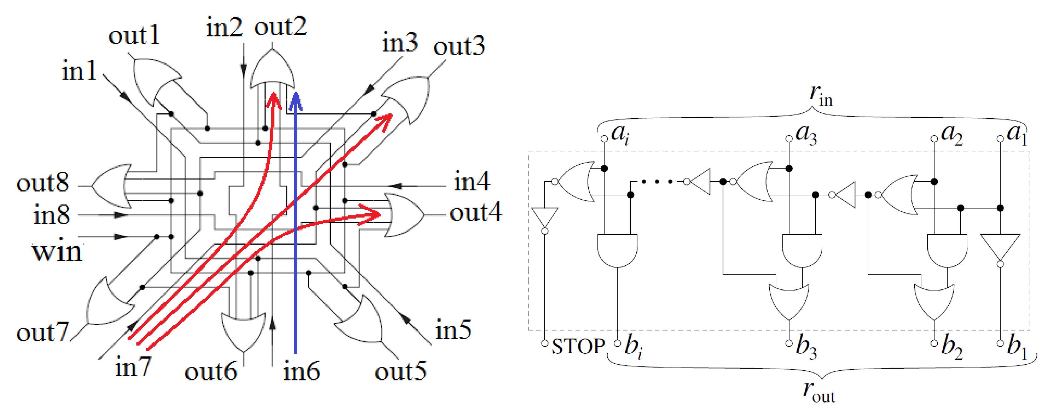
A state-of-the art neighborhood mechanism with the ability to determine the neighboring neurons has been proposed by Macq, Verleysen et al. in [40]. It is a digital circuit, and thus it is a counterpart to our proposed solution. This circuit features a simple structure, in which only a few logic gates are used per each neuron in the SOM. However, it allows to activate the neighboring neurons at the distance of only one, which has a limited usage. This means that each neuron can have only one ring of neighboring neurons. In contrary to this approach, our circuit allows to obtain any neighborhood radius.

Another solution of this type, which may be compared with our circuit, is the one proposed by Li et al. in [41]. The authors of this work have realized an analog Gaussian neighborhood function (GNF). The circuit was verified only for small maps with four (2 × 2) neurons, with the neighborhood size of only one. The output current represents the neighborhood distance ${\left({\rho }_c{\rho }_i\right)}^2$, in which the ${\rho }_c$ signal identifies which neuron is the winner, while ${\rho }_i$ may be considered as identifiers of particular neighbors. The identifiers are currents with constant values, specified before starting the learning process. For the map with four neurons, the constant analog signals are sufficient, as all distances equal one. In maps with larger numbers of neurons the values of the identifiers cannot be constant, as the distance to the winner may vary during the adaptation process. For this reason, a more sophisticated NM is still required to enable an implementation of larger maps.

The solution proposed in [41], as well as remaining two described above, show that the implementation of the neighborhood mechanism with large neighborhood radius, in the neural networks working in parallel in hardware is not trivial. We have taken up this topic due to a large potential of such implementations in practical applications requiring miniaturization and high computing power. In this work, we proposed a significant optimization of our former circuit, by the above-mentioned reduction of the number of multiplication operations. Details are presented in following parts of this paper.

In the literature one can also find examples of using field programmable gate arrays (FPGAs) to implement the SOM. However, they are not comparable with the proposed transistor-level implementations in terms of the structure, power dissipation and data rates. In general, there are different assumptions in these approaches. One of the objectives in case of the FPGA realization is fast prototyping, while power dissipation is of secondary importance. In case of the ASIC implementation the situation is quite opposite.

3. Design and Test Methodology

The proposed NM should not be considered as a separate block, as in the presented implementation it closely cooperates with other components that include the adaptation mechanism (ADM). For this reason, the NM has been designed in such a way so that it supports the adaptation block. Before we move more deeply into details of the proposed solution, we have to present some necessary basics of the SOM and constraints related to its hardware realization. The methodology presented in this section covers such issues as the choice of the SOM architecture (parameters, particular blocks) and quantitative methods of assessment of the learning process, for different values of crucial parameters of the SOM.

3.1. Basics of Kohonen Self Organizing Maps

The Kohonen SOM learning algorithm is divided into the, so-called, epochs. During a single, eth, epoch all learning patterns $\mathit{X}$ from an input (learning) data set are presented to the NN in a random sequence. The epochs are composed of learning cycles, l, during which particular learning patterns $\mathit{X}$ are fully processed. In a single lth cycle the NN computes the distances between a given pattern and weights vectors $\mathit{W}$${}_j\left(l\right)$ of all neurons. At the next step of a given cycle, the winning neuron is determined. It is the unit for which the distance is the smallest. This operation is followed by the adaptation of the weights of the winning neuron and it’s neighbors, as follows:

$$W_j(l+1)=W_j\left(l\right)+\eta \left(e\right)·G(R,d(i,j))·[X\left(l\right)-W_j\left(l\right)]$$

(1)

In the formula above, $\eta \left(e\right)$ is the learning rate, which is constant for a given learning epoch. The values of $\eta \left(e\right)$ for particular neighboring neurons are modified according to a neighborhood function $G\left(\right)$, depending on a distance, $d(i,j)$ (in the map space) between the winner, i, and a given neighbor, jth. The R parameter in the $G\left(\right)$ function is the neighborhood range. All neurons in the map form rings around the winner. However, only the rings for which $d(i,j)\le R$ are treated as considerable neighborhood of this winning neuron. Before starting the learning process, the radius R is set to a maximum value, $R_{\max }$). During the adaptation process it gradually diminishes to zero, which shrinks the neighborhood range.

3.2. Topology of Self-Organizing Map

One of the important parameters of the SOM is its topology that determines the number of neighbors of particular neurons. In the literature one can find three typical topologies [12] with 4, 8 (rectangular) and 6 (hexagonal) neighbors. In our works we refer to them as Rect4, Rect8 and Hex [22]. This parameter has a noticeable impact on the learning process. In our former works we investigated the influence of this parameter on the learning process. A general calculation scheme, given by (1), is independent of the topology of the SOM.

3.3. Neighborhood Function

Another important parameter is the neighborhood function (NF). As can be seen in Figure 3, the neighboring neurons form rings around the winning neuron. The distance between a given ring and the winner, in the map space, is denoted as $d(i,j)$. The NF determines the intensity of the learning process at a given ring of neighbors. Several neighborhood functions $G(R,d(i,j\left)\right)$ can be used in the adaptation process described by (1). The simplest one is the classical rectangular neighborhood function (RNF), in which all neighbors are adapted with equal intensities. This function is defined as follows [12]:

$$G(R,d(i,j))=\left\{\begin{array}{cc}1\hfill & \mathrm{for} d(i,j)\le R\hfill \\ 0\hfill & \mathrm{for} d(i,j)>R\hfill \end{array}\right.$$

(2)

In our former investigations we have shown that the RNF is sufficient for the maps with up to 200–250 neurons. Much better results have been achieved by using the GNF. For comparable learning data sets this function allowed us to properly train the maps with more than 1500 neurons. The GNF is expressed as follows:

$$G(R,d(i,j))=exp\left(-\frac{d^2(i,j)}{2R^2}\right)$$

(3)

This function is difficult to implement at the transistor level, as the exponential and the division operations require complex circuits. The problem becomes serious in parallel SOMs, in which each neuron is equipped with own GNF block. Taking this into account, in our former works, we considered a substitution of the GNF with a much simpler TNF. In our transistor level implementation the TNF uses only a single multiplication and a simple bits shift operations [25]. It may be expressed as follows:

$$G(R,d(i,j))=\left\{\begin{array}{cc}-a\left({\eta }_0\right)·(R-d(i,j))\hfill & \mathrm{for} d(i,j)\le R\hfill \\ 0\hfill & \mathrm{for} d(i,j)>R\hfill \end{array}\right.$$

(4)

The $a\left(\right)$ parameter that results from the steepness of the TNF, as well as the learning rate of the winner, ${\eta }_0$, are decreased after each epoch.

We performed investigations that aim at a verification whether the TNF can be used as a substitute for the GNF. The obtained results (learning quality) for the TNF are comparable with the GNF, while the circuit complexity is in this case at the level of only 5–10% of the GNF. Selected illustrative simulation results are shown in Section 3.5. In these investigations we compared the overall learning process for the maps with the numbers of neurons in-between 16 and 1600. For both described NFs, the number of iterations needed to obtain an optimal distribution of neurons was similar for a given learning data set. Thus we can say that the total energy consumed by the SOM in case of using the TNF is less than in case of using the GNF.

In the literature, one can find hardware realizations of the Gaussian function. Such function is used, for example, in the realizations of the Radial Basis Function Neural Networks (RBF-NNs). NNs of this type are mainly realized using the FPGA platforms [42,43,44,45]. Such realizations, despite some advantages (time and cost) suffer from several limitations. One of them is relatively high power consumption versus data rate. However, it is not the most important parameter in this case. A second limitation, especially when compared to ASIC implementations, is a fully synchronous operation that increases the computation time. As a result, the data rate to some degree depends on the number of neurons in this case.

In our former works, we also considered the use of the exponential neighborhood function. This function is hardware efficient, as it requires only shifting the bits at following rings of neighbors. However, in the simulations performed in the software model of the SOM, the results comparable to those obtained for the TNF and the GNF functions were not achieved. For this reason, we do not further consider this function in this work.

3.4. Assessment Methods of the Quality of the Learning Process

Various criteria have been proposed to objectively evaluate the quality of the learning process of the SOMs. To most popular belong the quantization and the topographic errors [46,47,48]. In our investigations, we usually use the criteria proposed in [47]. They allow for the evaluation of the learning process in two ways. One of them focuses on the quality of the vector quantization, while the second one on topographic mapping. All these criteria have already been presented in our earlier works [22,25,49]. Since we also use them in this work, to facilitate reading the paper, we briefly present them in this Section.

The quantization error may be assessed with the use of two measures. The quantization error, defined below, is one of them:

$$Q_{\mathrm{err}}=\frac{1}{m}\sum _{j=1}^m\sqrt{\sum _{l=1}^n{(X_{j,l}-W_{i,l})}^2}$$

(5)

In this equation, the m parameter is the number of the learning patterns in the input data set. The $Q_{\mathrm{err}}$ indicates how well the SOM approximates the input data set (vector).

The second measure related to the quantization quality is a ratio between the number of the, so called, dead (inactive) neurons (PDN) and a total number of neurons in the map (percentage). The dead neurons are the units that take part in the competition, but never won. In this way, after completing the learning process they are not representatives of any data class.

The two errors above do not allow to assess the topological order in the SOM. For this reason, the quality of the topographic mapping has to be assessed using other measures [47].

One of them is a Topographic Error, $E_{\mathrm{T}1}$, proposed by Kohonen [12,48]. It is defined as follows:

$$E_{\mathrm{T}1}=1-\frac{1}{m}\sum _{h=1}^m\lambda \left(X_h\right)$$

(6)

The value of the $\lambda \left(X_h\right)$ factor is equal to 1 in the situation, in which for a given learning pattern $\mathit{X}$ two neurons whose weight vectors that are the closest to this pattern are also direct neighbors in the map. In other case the value of $\lambda \left(X_h\right)$ is zero. This means that the lower is the value of $E_{\mathrm{T}1}$, the SOM preserves a given topology of the map in a better way [48].

The remaining criteria do not need the information on the distribution of the patterns in the input data space. The procedure of the second criterion, $E_{\mathrm{T}2}$, starts with we computation of the Euclidean distances between the weights vector of an $\rho$th neuron in the map and the weights of remaining neurons. Then it is checked if all p direct neighbors of a given neuron $\rho$ are also its nearest neighbors in the input (Euclidean) data space. Let us assume that a given neuron $\rho$ has $p=\left|N\right(\rho \left)\right|$ direct neighbors. The value of the p parameter depends on the topology of the map i.e., the maximum possible number of direct neighbors of a given neurons. That $g\left(\rho \right)$ function returns the number of direct neighbors that are also in the closest proximity to neuron $\rho$ in the input data space. For P neurons in the SOM, the $E_{\mathrm{T}2}$ factor may be thus defined as follows:

$$E_{\mathrm{T}2}=\frac{1}{P}\sum _{\rho =1}^P\frac{g\left(\rho \right)}{\left|N\right(\rho \left)\right|}$$

(7)

In an optimal case, $E_{\mathrm{T}2}=1$.

The last criterion, $E_{\mathrm{T}3}$, from the topographic group requires building around each neuron, $\rho$, the Euclidean neighborhood. This neighborhood can be imagined as a sphere in the input data space with the radius:

$$R\left(\rho \right)=\underset{s\in N\left(\rho \right)}{max}\left|\right|X_{\rho }-X_s\left|\right|$$

(8)

where $X_{\rho }$ is the weights vector of a given $\rho$th neuron, while $X_s$ are weights vectors of particular direct neighbors of the neuron $\rho$. For each $\rho$ we calculate the Euclidean distances between a given neuron and its $p=\left|N\right(\rho \left)\right|$ direct neighbors. The $R\left(\rho \right)$ parameter is a radius that may be understood as a maximum value taken form a given set $\rho$ containing p values. In the next step, for particular neurons in the map, we count the number of neurons that are not their closest neighbors ($s\notin N\left(\rho \right)$), while being located inside the sphere with the radius $R\left(\rho \right)$. For these neurons $\left|\right|X_{\rho }-X_s\left|\right|<R\left(\rho \right)$.

The $E_{\mathrm{T}3}$ criterion may be expressed as follows (its optimal value is 0):

$$E_{\mathrm{T}3}=\frac{1}{P}\sum _{\rho =1}^P\mid \left\{s|s\ne \rho ,s\notin N\left(\rho \right),||X_{\rho }-X_s\left|\right|<R\left(\rho \right)\right\}\mid$$

(9)

3.5. A Comparative Study for Particular Neighborhood Functions

In this part, we present selected results obtained on the basis of simulations in the software model of the SOM for various combinations of key parameters related to this type of NN. As can be observed, the TNF is a good substitute of the GNF. To test the SOM, we used data sets composed of two-element learning patterns distributed over the 2-dimensional (2-D) input data space. Such data sets facilitate the illustration of the quality of the learning process [47,48]. They are divided into n data classes. Each class consists of the same number of the patterns. This approach facilitates the comparison of the learning results of the SOM for different combinations of key parameters of such networks [48]. To enable a direct comparison of the results, the maximum values in particular coordinates of the input space are fitted to the number of neurons in the map. For an example SOM containing 64 neurons (8 × 8 grid) the values in both coordinates are in the range from 0 to 1. For the map with 256 neurons (16 × 16 grid) the values are in the range in-between 0 and 2. As a result, independently on the sizes of the map, the minimum (optimal) value of the quantization error ($Q_{\mathrm{err}}$) is always equal to $0.016$. The optimal values of remaining parameters (PDN, $E_{\mathrm{T}1}$, $E_{\mathrm{T}2}$ and $E_{\mathrm{T}3}$) are equal to 0, 0, 1 and 0, respectively. The non-zero value of the quantization error results from a selected distribution of input pattern around centers of particular data classes in the input data space.

On the basis of the results shown in Figure 4 and in

Table 1. The quality of the learning process treated as a function of the initial neighborhood range $R_{\max }$, for the RNF, GNF and TNF (selected results).

Map Sizes: 6 × 6
Rmax	Qerr			PDM			ET1			ET2			ET3
	RNF	TNF	GNF	RNF	TNF	GNF	RNF	TNF	GNF	RNF	TNF	GNF	RNF	TNF	GNF
0	28.5	28.5	28.5	16.7	16.7	16.7	0.794	0.794	0.794	0.286	0.286	0.286	19.3	19.3	19.3
1	16.2	16.2	16.2	0	0	0	0	0	0	1	1	1	0	0	0
3	16.2	16.2	16.2	0	0	0	0	0	0	1	1	1	0	0	0
Map sizes: 12 × 12
Rmax	Qerr			PDM			ET1			ET2			ET3
	RNF	TNF	GNF	RNF	TNF	GNF	RNF	TNF	GNF	RNF	TNF	GNF	RNF	TNF	GNF
0	22.3	22.3	22.3	8.33	8.33	8.33	0.875	0.875	0.875	0.143	0.143	0.143	91.8	91.8	91.8
1	16.2	16.2	16.2	0	0	0	0	0	0	1	1	1	0	0	0
6	22.1	16.2	24.9	1.39	0	6.25	0	0	0.06	0.96	1	0.812	0.306	0	4.05
Map sizes: 18 × 18
Rmax	Qerr			PDM			ET1			ET2			ET3
	RNF	TNF	GNF	RNF	TNF	GNF	RNF	TNF	GNF	RNF	TNF	GNF	RNF	TNF	GNF
0	19.8	19.8	19.8	4.94	4.94	4.94	0.852	0.852	0.852	0.116	0.116	0.116	204.6	204.6	204.6
1	16.2	16.2	16.2	0	0	0	0	0	0	1	1	1	0	0	0
7	24.3	16.2	28.3	1.23	0	2.78	0.001	0	0.004	0.95	1	0.919	0.420	0	0.846
Map sizes: 24 × 24
Rmax	Qerr			PDM			ET1			ET2			ET3
	RNF	TNF	GNF	RNF	TNF	GNF	RNF	TNF	GNF	RNF	TNF	GNF	RNF	TNF	GNF
0	18.9	18.9	18.9	3.65	3.65	3.65	0.908	0.908	0.908	0.088	0.088	0.088	358.2	358.2	358.2
1	16.2	16.2	16.2	0	0	0	0	0	0	1	1	1	0	0	0
4	25.1	16.2	25.6	2.08	0	3.30	0.021	0	0.009	0.893	1	0.924	1.84	0	1.14

one can conclude that for the TNF and the GNF the learning process leads to similar results. On the other hand, the results obtained for the RNF are comparable to those obtained for the TNF and the GNF only for small maps composed from up to 64 neurons. If larger maps have to be applied, the optimal solution is the TNF.

To make the comparison of particular NFs more transparent we illustrated the obtained results in Figure 5. The histograms illustrate the number of cases, for which the map became properly organized ($Q_{\mathrm{err}}=16.18\times {10}^{-3}$) for particular NFs, as a function of the map sizes. The largest map for which the optimal values of the five assessment criteria described above have been achieved was the map with $28\times 28$ neurons working with the TNF.

More detailed simulation results for three network topologies (Rect4, Rect8, Hex), different datasets (2D and 3D), different distance measures and various initialization methods of the weights that confirm the above conclusions are shown in our previous works [22,25,49].

4. The Proposed Cocnept of the Digital NM

4.1. Previous Concept of the NM

To present the new proposed solution of the neighborhood mechanism, neighborhood function and the adaptation module in a proper perspective, it is necessary to briefly present our former concept of the neighborhood mechanism [22]. In parallel SOMs realized in hardware, in which each neuron is realized as a separate circuit, the neighborhood mechanism creates concentric rings of neighbors around each of the neurons in the map, as shown in Figure 3.

Particular neurons communicate with each of its neighbors throughout the EN and the r signals. The important issue was how to effectively determine at the transistor level, which neurons belong to particular rings of neighbors for any neuron in the map. This problem has been solved by two blocks named EN_PROP and R_PROP, proposed in [22]. In that solution, the winning neuron sends the EN (enable) signal in all directions. As a result, all its direct neighbors (eight in the presented case) are activated. These neurons in turn propagate the EN signal to the next ring (16 neurons). In this case, however, the signal can be propagated only in selected directions, to avoid the situation in which, for example, the EN signal returns to the winning neuron. This is assured by the asynchronous EN_PROP block that is composed only of logic OR gates. For the winning neuron the win signal equals ‘1’, resulting in all enable out signals becoming active. The win signal is the input signal to all OR gates. In other neurons the win signal equals ‘0’. Each neuron receives the enable input signal from only one direction and, as an answer, activates its only selected outputs. If the enable signal comes from any diagonal direction it activates three neurons at the opposite side, while if the signal comes from horizontal or vertical directions it activates only one neuron. It is illustrated in Figure 6 (top). For example, if in7 equals ‘1’ then out2, out3 and out4 outputs become active. However, if in6 is active, it activates only out2 output. The overall propagation process is fully asynchronous and parallel in all neurons and thus very fast. The propagation of the enable signal resembles a concentric wave.

The second problem is how to stop the propagation of the EN signal at a given ring of neighbors. This is realized by the use of the R_PROP block, which asynchronously decrement the obtained multi-bit signal r by 1. Each neuron in the map holds the information about the assumed neighborhood range, R. If a given neuron becomes the winner, it decrements this value and then propagates it, throughout the r signal, to all its direct neighbors in parallel with the EN signal. Each of its neighboring neurons also decrements this signal and further propagates. To avoid conflicts, each neuron receives the r signal only from this direction for which the EN${}_{\mathrm{in}}$ signal is active. This is realized by switches controlled by the enable in signals, visible in Figure 6 (bottom). If at a given ring of neighbors the r signal becomes zero, the further propagation of the enable and the r signals is blocked.

The r signal plays also an additional role in the proposed solution. This signal is the input to the NF block in each neuron. The distance, $d(i,j)$, of any neuron to the winning neuron equals $R-r$. For this reason, the $a\left({\eta }_0\right)·(R-d(i,j))$ term in (4) reduces to $a·r(i,j)$. As a result, (1) for the TNF can be expressed as:

$$W_j(l+1)=W_j\left(l\right)+\eta \left(e\right)·a·r·[X\left(l\right)-W_j\left(l\right)]$$

(10)

Note that the adaptation process in this form requires three multiplication operations. In this formula the coefficients $\eta \left(e\right)$ and a are constants in a given learninxg epoch e and thus can be replaced with a single factor that is the product of them, as follows:

$$\eta \left(k\right)·a=E/D$$

(11)

Since a and $\eta$ are less than one, the term above is a fractional number also less than one. To simplify the division operation, the value of the denominator is selected to be one of the powers of 2. As a result, this operation can be realized simply by shifting the bits to the right by a given number of positions. Formula (11) allows to express (10) as follows:

$$W_j(l+1)=W_j\left(l\right)+E·r·[X\left(l\right)-W_j\left(l\right)]/D$$

(12)

This is instrumental to reduce the number of multiplications by one. At the transistor level, the shifting of the bits is a simple operation that requires only an asynchronous and passive block of switches.

4.2. Proposed Improvements of the NM

Reduction of the number of the multiplication operations by one does not solve the problem. Two multiplications require a 2-phase clock that control the computing process of (12). There is also a need to store the intermediate product of the first multiplication before the second operation of this type. That requires an additional memory in each neuron. In this Section we present a novel solution that further strongly simplifies the overall calculation scheme. The new solution allows to avoid using the mentioned clock and memory blocks, and thus has a substantial impact on further optimization of he overall SOM. This is what has been said earlier in this work, that even a small reduction of the complexity in one of the blocks of the NN has a very positive impact on the structure of the overall network, by helping to reduce the complexity of other blocks.

To highlight the novelty of the proposed solution, we introduce a new variable $\beta$. This variable for the winning neuron and subsequent kth ring of neighbors, respectively, is defined as follows:

$${\beta }_0=E·R$$

(13)

$${\beta }_k=E·(R-k)=E·R-E·k={\beta }_0-E·k$$

(14)

where the k variable is equal to the distance, d, between the winning neuron and a given ring of neighbors.

All $\beta$ variables are integers. Before each eth learning epoch, consisting of multiple cycles l, each neuron receives new values of the variables ${\beta }_0$, E and D. Note, that for any two adjacent neurons, (14), can be expressed as:

$${\beta }_k={\beta }_{k-1}-E$$

(15)

In other words, the difference between the ${\beta }_{k-1}$ and ${\beta }_k$ always equals E. For this reason, in the new approach instead of propagating the multi-bit r signal, we propagate the multi-bit ${\beta }_k$ variable between adjacent rings of neurons. The neurons in a given ring receive from the previous ring the ${\beta }_{k-1}$ signal, from which they always subtract the E variable. To make it possible, the R_PROP block in the new solution has been substituted by a multi-bit full subtractor. The subtractor also operates asynchronously, as it was in the case of the R_PROP block.

Taking the calculated value of the $\beta$ signal, the updates of the weights are calculated as follows:

$$\Delta W=[{\beta }_k·(X\left(l\right)-W_j\left(l\right))]/D$$

(16)

As a result, (1) can be expressed as follows:

$$W_j(l+1)=W_j\left(l\right)+\Delta W$$

(17)

where:

$${\beta }_k/D=\eta \left(\right)·a·r$$

(18)

This allowed us to reduce the number of the operations in both the neighborhood mechanism and partially in the adaptation block to only three, with only a single multiplication among them. Remaining two operations are a single subtraction and a single bits shift. All these operations are performed fully asynchronously. This eliminates the need of using intermediate memory, while the calculation of the Equation (17) requires only 2-phases clock. In the 1st phase the circuit calculates the $[{\beta }_k·(X\left(l\right)-W_j\left(l\right))]/D$ term, while in the 2nd phase the weights are updated by the addition of this term. This is one of main advantages of the proposed solution over the previous approach.

4.3. Transistor Level Implementation of the NM

The proposed circuit that performs all operations given by Equations (15) and (16) is shown in Figure 7. The Figure illustrates the operations performed at the connection between any two pairs of adjacent neurons (adjacent rings of neighbors). For the winning neuron, the win signal equals ‘1’. This signal closes those switches that provide the $R·E$ signal to the subtraction circuit (substitute of former R_PROP block), realized as a multi-bit full subtractor (MBFS), as well as to an asynchronous multiplier (AMULT). For the winning neuron the k index equals 0 and increments at each following ring of neurons by 1. The MBFS located in the winning neuron subtracts the constant parameter E from the $R·E$ signal. The resultant, $(R-1)·E$, signal is provided to its direct neighbors at first ring. Each following ring also subtracts the E constant from the received signal. This operation is repeated as long as the resultant signal becomes ≤ 0.

The MBFS is composed of a chain of 1-bit full subtractors (1BFS), as shown in Figure 8. The $e_1$, $e_2$, ⋯, $e_n$ signals are bits of the E constant, while the $b_1$, $b_2$, ⋯, $b_n$ signals are following bits of the $\beta$ signal. The situation in which the $\beta -E$ is less than 0 is signalized by the non zero borrow out bit at the most significant 1BFS (${\mathrm{B}}_{\mathrm{o}n}=1$).

The multiplier, shown in Figure 9, operates in two’s complement notation, as the $X\left(l\right)-W_j\left(l\right)$ vector may contain negative elements. The multiplier is realized as an asynchronous binary tree (BT) circuit, composed of asynchronous multi-bit full adders (MBFAs). The BT multipliers are more complex (in terms of the number of transistors) than typically used shift-and-add circuits, however since the E signals are usually small, therefore a small number of MBFAs is sufficient. Figure 9 shows the multiplier for the 4-bits E signals ($E_{\max }=15$). In this case on two layers of the BT only three MBFAs are used.

The AMULT returns the product of the multiplication of the ${\beta }_{k-1}$ signal and the $(x_i\left(l\right)-w_{i,j}\left(l\right))$ term (for a given x and w pair). This signal is further divided by D factor. This operation is realized by shifting the bits by a given number of positions to the right, by the use of the asynchronous BSHIFT block. The chain of the AMULT and the BSHIF blocks provides an update of the corresponding weight for a given neuron. As a result, it can be said that the proposed circuit contains components of the neighborhood mechanism, the neighborhood function and one of the main components of the adaptation mechanisms. Note, that all these operations are performed fully asynchronously, which simplifies the circuit on one hand and speeds up the calculation process on another.

Figure 10 presents an idea of the adaptation block, which is an accumulator controlled by a simple 2-phases clock. It modifies the neuron weights by the signal received directly from the circuit shown in Figure 7.

The components of the new neighborhood mechanism has been recently implemented by the author in a prototype chip, realized in the CMOS 130 nm technology. One of the basic components that have been realized is the 1BFS, shown in Figure 11. The circuit is composed of 30 transistors, with the sizes (width and length) close to minimum values for this technology (0.5/0.13 $\mathsf{\mu }$m). The resultant chip area of a full MBFS is small. This solution allows to connect in an asynchronous chain any number of such blocks. That is essential from the point of view of the proposed neighborhood mechanism.

5. Verification of Implemented Neighborhood Mechanism with Neighborhood Function

It is worth pointing to the process of designing such circuits as described in the paper. In case of the ASIC design, the so-called time to market is substantially longer than in case of software projects. Design of such NNs is a complex task, as after the fabrication no changes are possible. The design process requires comprehensive simulations to check as many scenarios as possible to make the fabricated chip a universal solution. On one hand, the circuit has to be tested in terms of its functionality. One need to check if the algorithm is effective for selected classes of problems. At this stage the verification process is similar as in case of typical software projects. However, here an additional verification phase has to be carried out. The project of the chip has to be physically tested, before being sent to fabrication. This phase is very time consuming. The neural network can be composed of over a million transistors. A single transistor level simulation in Spice can last up to a week, while even several hundred of such simulations may need to be carried out before the fabrication phase. The simulations are usually performed in parallel on many computers. The circuit has to be robust against supply voltage, process and temperature variation (PVT corner analysis).

One of major limitations is the fact that in case if the project would need to be modified, it is necessary to perform a new testing procedure and to fabricate a new hip prototype.

We tried to reduce the impact of the described limitations by implementing built-in mechanisms that allow for a reconfiguration of the chip to some extent. For example, one can program the size of the network (number of neurons), of course, up to the values foreseen at the design stage, as well as the range of the neighborhood mechanism, the values of particular coefficients that impact the learning process of the NN, etc. Nevertheless, testing these mechanisms was also time-consuming, because it was necessary to check out the scope of particular parameters. For the comparison, in case of the software solutions, when one observes the absence of project optimality, relatively simple corrections of the program code are possible.

Taking the above into account, the proposed circuit has been verified in two ways. First, transistor level simulations were performed in the CMOS 180 nm technology, to determine a better insight into such parameters, as power dissipation, attainable data rates, robustness against variation of external parameters that include environmental temperature and supply voltage. Simulations allowed to verify the proposed concept for various signal resolutions (in bits).

After the simulation phase, the circuit has been redesigned and implemented in a prototype chip, realized in the CMOS 130 nm technology. The chip after the fabrication was the subject of detailed laboratory measurements. Both types of tests are presented in this section, below.

5.1. Simulations of the Proposed Circuit

Detailed simulations show that the proposed neighborhood mechanism is very fast, as the delay between two adjacent rings of neurons equals only the delay of a single subtraction circuit. Selected simulation results performed for the CMOS 180 nm technology are shown in Figure 12 and Figure 13. Particular signals have different resolutions, as follows: x and w are 16 bit signals, while D and $\beta$ are 5-bit signals. The $|x-w|$ operations do not need to be performed at this stage, as these terms are already determined during the calculation of distances between particular neurons and input learning patterns, at the beginning of each learning cycle. These terms are then stored in separate memory blocks and directly used in Equation (17).

In this example case, the E signal in this case equals 6. Figure 12 shows that the delay of a single ring of neurons is less than 0.5 ns. This in practice means that all neurons in the SOM receive their own values of the $\beta$ signal almost at the same time, thus the adaptation process is performed in parallel in the overall SOM.

It can be observed in Figure 12 that the T1 time is longer than remaining delay times. This is due to the fact that in the asynchronous operation of the proposed system, while the outputs of one block have not yet established, they are already driving the next blocks in the chain.

To verify the robustness of the proposed solution we performed a series of simulations for different values of the environmental temperature, for different values of the supply voltage and for several transistor models, namely: typical (TT), fast (FF), and slow (SS). Such analysis, called corner analysis, is commonly used in commercial projects before the chip fabrication. Selected results of this analysis are shown in Figure 14. The investigations have shown that the circuit operates properly in a wide range of the tested parameters. The supply voltage varied in the range from 0.8 to 1.8 V, while the temperature in-between −40 ${}^{\circ }$C and 100 ${}^{\circ }$C. The circuit worked properly for each tested case. The only difference in behavior was observed in delay introduced by the proposed circuit. For the worst case scenario (SS/100 ${}^{\circ }$C) the delay did not exceed 0.4 ns, while typically it was about 0.3 ns. The presented results show that even if the size of the neighborhood is large (10–20 rings) the overall mechanism is relatively fast, introducing the total delay not greater than 10 ns.

A further improvement in terms of data rates can be achieved if the proposed circuit is implemented in more dense technologies that offer much shorter switching times of transistors and logic gates. The presented implementation in the 180 nm process results form the fact that other SOM components are already realized in this process.

Another important parameter is the power dissipation. The circuit consumes the energy only during switching. Diagram of Figure 13 shows the supply current. During the calculation session an average current does not exceed 1 mA, which for a given calculation time in a single session allows to assess the energy consumption to be equal to about 1 pJ. The presented results are shown for 6 neurons in the chain, so a single neuron consumes only about 200 fJ.

Particular components of the proposed circuit have been additionally verified by means of laboratory tests of the prototype chip, mentioned above.

5.2. Measurements of the Prototype Chip

Selected and elaborated measurement results are shown in Figures. Particular Figures illustrate:

• Figure 15 Inputs and outputs of the circuit as binary signals—11 input bits and 11 output bits.
• Figure 16 4-bit In1 and In2 input signals recalculated to decimal format. Due to the limitations in the number of pads, the TNF circuit has been verified for 4-bit signals. The In1 and In2 input signals are counterparts to ${\beta }_k$ and $|x-w|$ signals, respectively.
• Figure 17 Output signals of the TNF circuit, recalculated to decimal format and carry out signals, as explained below in more detail.

The realized TNF circuit performs the operation given by expression 19 below, i.e., a direct realization of Equation (16), in which the multiplication of the $|x-w|$ term by the ${\beta }_k$ signal is followed by division by the D signal.

$$\mathrm{Out}=(\mathrm{In}1·\mathrm{In}2)/D$$

(19)

The Out signal is the counterpart to the $\Delta \mathit{W}$ signal in (16). The In1 (${\beta }_k$) input represents the $\eta \left(e\right)·G(R,d(i,j\left)\right)$ term in Equation (1). The division by the D signal is performed by shifting the bits in the computed product In1·In2.

The In1 and In2 input signals are provided to i00–i03 and i04–i07 binary inputs of the prototype chip, respectively. The $Din$ signal is provided to the chip as a 2-bit signal, to binary inputs i08–i09. Inside the chip, the signal is decoded as follows:

$Din=00\to$ (d1 = 1, d2 = 0, d3 = 0, d4 = 0) →$D=1$

$Din=01\to$ (d1 = 0, d2 = 1, d3 = 0, d4 = 0) →$D=2$

$Din=10\to$ (d1 = 0, d2 = 0, d3 = 1, d4 = 0) →$D=4$

$Din=11\to$ (d1 = 0, d2 = 0, d3 = 0, d4 = 1) →$D=8$

The d1–d4 signals are further provided to particular groups of switches inside the circuit responsible for shifting the bits, thus performing the division operation.

The i10 input terminal is not used by the TNF circuit. This input is used to switch over the overall chip between two modes, as follows:

• for i10 = ‘1’ the chip is in the programming mode,
• for i11 = ‘0’ the chip is in a typical operation mode.

In the programing mode (in-between 0 and 1000 ns), the remaining inputs have another meaning, so the output signals of the chip are in this period insignificant from the point of view of the operation of the TNF block. The i00–i09 signals are in this mode used as addressing lines of configuration memory cells, as the binary values to be stored in particular cells and a latch (storing) trigger.

After the 1000 ns period, the TNF block is tested in regular cycles lasting 400 ns each. Each cycle is further divided into four steps (100 ns each). In particular cycles the In1 and In2 signals are constant, however, in particular steps of each cycle the D signal varies in such a way, that the product In1·In2 is shifted by 0, 1, 2, 3 bits to the right. This translated into the division by 1, 2, 4 and 8, respectively. As can be observed in Figure 17, the output signal decreases accordingly. The values at the output of the TNF are natural numbers, so after the division the result is automatically rounded toward smaller natural value (a floor operation).

The output binary signals, o00–o10, need to be interpreted in an appropriate way. The o00–o07 terminals provide subsequent bits of the 8-bit output signal of the TNF. The remaining three more significant bits o08, o09 and o10 represent carry out bits from particular summing circuits inside the TNF block. The multiplier is built as an asynchronous binary tree with two layers, shown in Figure 9. The first layer is composed of two MBFAs. Each of them has its own carry out terminal, denoted in Figure 17 as CoL1_1 and CoL1_2, respectively. At the second (last in this case) layer of the tree a single MBFA is used, with its own carry out terminal, denoted as CoL2.

5.3. Comparison with Previous Version of the NM

5.3.1. Computation Time

The reduced hardware complexity of the new solution presented in this work has a positive impact on several factors and features of the overall SOM. The subtraction circuit used instead of the former R_PROP block features a similar delay, so the part of the proposed circuit responsible for the determination of distances between the winning neuron and particular rings of neighbors is as fast as in the former solution. The new approach, however, allows for substantial improvements in other modules of the SOM. Due to only a single asynchronous multiplication operation, the circuit used for the calculation of the NF, as well as of the updates of the neuron weights is strongly simplified.

The previous solution, described by Equations (12) and (18), could have been implemented in two ways. One of them required a single asynchronous multiplier, however due the multistage multiplication intermediate products had to be stored in an additional memory block. This approach required also a control clock. Since the memory does not require a large number of transistors (10 per a single bit), the complexity of the overall circuit was comparable. In this case, however, the computation time of the updates of the neuron weights was even over three times greater than in the current approach. Another possibility was the use of two asynchronous multipliers connected in series. In this case, the computation time was about 60% longer, but this part of the circuit contained more than twice as many transistors as in the current solution.

In the first described approach of the previous solution, the clock generator (based on a D-flip flop) was composed of about 40 transistors, while the memory block used 160 transistors, for an example case of 16-bit of the resolution of the x and w signals. In the second approach, the additional multiplier requires more than 2000 transistors per neuron, even for relatively small resolution of the input signals of 8-bits.

In the new solution the R_PROP circuit has been replaced with the MBFS. This means that each bit requires 10 additional transistors, i.e., 160 transistors per a single neuron for the example resolution of 16 bits.

Since the new solution is fully asynchronous, therefore the calculation of a single $\eta \left(e\right)G(R,d(i,j))(x_i\left(l\right)-w_{i,j}\left(l\right))$ signal requires less than 3–5 ns (data for the CMOS 130 nm technology). In the previous approach this time was longer even by 50%, for the option with two multipliers, or even three times longer for the first option with the intermediate memory and the controlling clock.

5.3.2. Energy Consumption

The main advantage of the actual structure of our novel approach is the elimination of two multiplication operation per each neuron, which are energy-intensive, especially for input values with higher resolution (in bits). The multiplication operation consumes several dozen times more energy than e.g., the addition or the subtraction operations. In addition, the division operation, performed here as shifting the bits with the use of a commutation field of switches, requires little energy. In the proposed solution the multiplication operations have been substituted with the subtracting one and thus the substantial energy savings. So, if one multiplication operation is eliminated, the energy consumption of the neighborhood mechanism is at least by half lower. It is worth to add, that a single multiplication operation, assuming the use of a single multiplication block per neuron, means that there is no need to keep an intermediate result in the memory. This eliminates the need of the data storage operation that also consumes energy. Another benefit results from the fact that in the new approach the process of the propagating of the neighborhood signals, as well as the computing of the triangular function in all neighboring neurons in the SOM became fully asynchronous. This eliminated a clock generator that in the previous approach was used to control the described multiplication sequence, consuming energy.

On the other hand, the new solution uses subtraction circuits instead of the decrement circuit, which was used in our previous approach. This component consumes about 20% more energy than its counterpart used in our previous solution. However, this factor is insignificant as both the subtracting and the decrementing operations consume very low energy in the comparison with the multiplication one.

Summarizing, the energy consumption in the new approach (the neighborhood mechanism with the TNF) equals only about 30–40% of the energy consumed in the previous solution. We provide a range of values. This results from the fact that depending on the shape of the neighborhood function (the steepness of the triangle’s slopes), the subtraction circuits operate with numbers of different values, i.e., different numbers of logic gates have to be switched over in a given neuron. For larger values of the ${\beta }_k$ factor, the energy consumed per one operation can vary by 20%.

Figure 18 shows the energy consumption per a single neuron, for different supply voltages, 20 ${}^{\circ }$C, for three transistor models. As can be seen, in our previous approach the energy consumed by a single neuron equals about 3.5 pJ for the supply voltage of 1.8 V [22]. In our new solution the energy is about 35% lower.

5.4. Indications for Future Advancement of the Current Research

Due to the complexity of the described design process, it was not reasonable to fabricate the overall NN at this stage. In the paper, we focus on selected core blocks. These blocks have been successfully tested in the laboratory. The next step will be the implementation of a full neuron and a network with a limited number of neurons to enable full testing of the proposed neighborhood mechanism. Such a mechanism can only be tested on a larger number of neurons working together. The network size has an influence on the chip area. Here, unfortunately, the size of the implemented network will depend on access to appropriate funds.

One of the research directions will be checking the efficiency of the neural network in newer CMOS technologies. At this stage of the investigations, only simulations are planned. This results from financial issues. However, the NN is a digital system. For this reason, simulations to a large extent are reliable form of the verification. The circuit environment (e.g., temperature) can only change the computation time, which may not be a problem if an adequate margin is maintained.

It is also necessary to verify real values of the energy consumption. The simulations provide a good assessment, however real tests are needed to enable a design of the power block of the sensor.

6. Conclusions

In this work we presented a novel approach to the implementation of both the neighborhood mechanism and the neighborhood function, suitable for self-organizing maps realized at the transistor level in the CMOS technology. The proposed circuit additionally computes updates of the neuron weights, so it also substantially simplifies the adaptation mechanism.

In the comparison with our previous circuit of this type, the novel approach offers substantial improvements in such parameters as the circuit complexity, the computation time and the power dissipation. Since to our knowledge, there are no other similar solutions of this type reported in recent years, therefore we threat our former approach as a state-of the art reference solution. We found some FPGA implementations of the Kohonen SOM, however, realizations in FPGA and as an ASIC are not fully comparable, due to other assumptions and requirements.

In the new proposed approach, to determine the distance of a given neuron to the winning neuron, as well as the calculation of both the neighborhood function and the correction of the neuron weight, we need only three basic operations performed asynchronously: subtraction, multiplication and shifting the bits. The last operation corresponds to the division operation by an integer number, which is one of the powers of the number 2. All these components, as well as the overall TNF function, have been realized in a prototype chip fabricated in the CMOS 130 nm technology, and successfully verified by means of the laboratory measurements. Since particular intermediate signals are not available outside the chip, therefore the behavior of the proposed mechanism is additionally illustrated on the basis of transistor level simulations. That form in case of digital circuit is reliable, especially as we performed a full corner analysis for different values of process, voltage and temperature variation.

Considering the features described above, the neighborhood mechanism is able to determine distances between a winning neuron and its neighbors in a very short time. For an example case of 10 rings of neurons, all distances are computed in a time not exceeding 5–10 ns. Then, the time of calculating an update of a single neuron weight, in parallel in all neurons in the SOM, does not exceed 1–1.5 ns.