Abstract
Reliable transmission expansion planning is critical to power systems’ development. To make reliable and sustainable transmission expansion plans, numerous sources of uncertainty including demand, generation capacity, and fuel cost must be taken into consideration in both spatial and temporal dimensions. This paper presents a new approach to selecting a small number of high-quality scenarios for transmission expansion. The Kantorovich distance of social welfare distributions was used to assess the quality of the selected scenarios. A case study was conducted on a power system model that represents the U.S. Eastern and Western Interconnections, and ten high-quality scenarios out of a total of one million were selected for two transmission plans. Results suggested that scenarios selected using the proposed algorithm were able to provide a much more accurate estimation of the value of transmission plans than other scenario selection algorithms in the literature.
1. Introduction
The integrated electric utility, owning both generation and transmission, traditionally develops generation plans first and then plans the transmission necessary to support those generation plans, an approach consistent with the fact that generation investments are normally far more costly than the needed transmission investments. Today, however, there are organizations that own transmission only. There are also service companies, called regional transmission organizations in the U.S., that own no infrastructure, but are responsible for coordinating the planning function. Both of these organizations must solve the transmission expansion planning (TEP) problem under uncertainty regarding technology, quantity, location, and timing of generation investments [1,2,3,4]. Robust and stochastic optimization approaches are two major modeling techniques for transmission planning under uncertainty, which have their own strengths and limitations.
Robust TEP maximizes the performance of the power system under the worst case scenario, which is dependent on the transmission plan [5,6,7,8,9,10]. Most solution techniques for robust TEP consist of two iterative steps: one step identifies the worst case scenario for a proposed transmission plan, whereas the other proposes the most robust transmission plan against a pool of worst case scenarios. A major advantage of robust TEP is its robustness against worst case scenarios, which is especially desirable for enhancing long-term resiliency of power system infrastructures. The iterative algorithm also allows the model to efficiently identify worst case scenarios from an enormous solution space with a large number of (or even infinitely many) possible scenarios. On the other hand, this approach often tends to be over-conservative by focusing on the possibility and ignoring the probability of worst case scenarios.
Stochastic TEP addresses uncertainty with a very different philosophy. It maximizes the average performance of the power system under all scenarios, weighted by their probabilities of occurrence. As such, the optimal stochastic transmission plan finds a good balance between the (positive or negative) impact and the likelihood of all scenarios [11,12,13,14,15,16]. However, this approach also faces a dilemma. On the one hand, due to the numerous sources of uncertainty and long planning horizon, a large number of scenarios is necessary to realistically represent the complexity and uncertainty of the TEP problem. On the other hand, however, the computation time of most solution techniques is very sensitive to the number of scenarios, and many algorithms become intractable for even a few dozen scenarios. To address this dilemma, scenario generation and reduction techniques have been proposed, which attempt to identify a small set of high-quality scenarios that represent the whole set of scenarios [17,18,19,20,21].
An alternative approach is to use an iterative stochastic TEP model, which attempts to combine the advantages of robust and stochastic TEP approaches and to overcome their limitations. A major limitation of the stochastic TEP approach with scenario generation and reduction is the assumption that the set of selected scenarios will be a good representation of the whole set of scenarios for all transmission plans. This is analogous to identifying one scenario as the “worst case scenario” for all transmission plans in the robust TEP approach. The iterative model in robust TEP acknowledges the need for re-identifying a worst case scenario for each new transmission plan, until the pool of worst case scenarios is sufficiently inclusive of all worst case scenarios. Similarly, the iterative stochastic TEP model re-identifies a new set of high-quality scenarios for each new transmission plan until the pool of high-quality scenarios is sufficiently representative of the whole set of scenarios. A formal definition of high-quality scenarios is given in Section 2.2. Figure 1 highlights the conceptual differences among robust TEP, stochastic TEP, and the iterative stochastic TEP. The scope of this paper is the highlighted component for selecting high-quality scenarios.
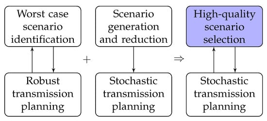
Figure 1.
Conceptual differences among robust transmission expansion planning (TEP) (left), stochastic TEP (middle), and the iterative stochastic TEP (right) models.
Scenario generation and reduction has been a topic of great interest in the power systems literature. Most existing methods use clustering [19,22,23,24] or sampling methods to reduce the number of scenarios from a randomly generated initial set. In a recent review article, Park et al. [25] compared four methods for scenario reduction using a two-stage stochastic transmission planning model, including random sampling, importance sampling [26], the distance-based method [17,27,28], iterative scenario reduction approaches, and stratified scenario sampling [25]. They used these methods to reduce a whole set of 20 scenarios to smaller subsets and compared their pros and cons. Other methods also include extended and improved initial-center-refined and weighted k-means [21], data-driven [29], forward selection [20], moment-based [18,30,31], and objective-based [32,33] approaches.
The proposed scenario selection approach in this paper differs from previous methods for scenario generation and reduction in three major ways. First, we generate scenarios with explicit consideration of temporal and spatial correlations, including generation investment and retirement decisions in response to demand, fuel cost, and transmission capacity. Second, we use the Kantorovich distance of social welfare distributions to assess the quality of the selected scenarios. Third, a different subset of high-quality scenarios is selected for each transmission plan candidate. In comparison, most existing methods in the literature ignore the correlations among the scenarios, select a subset of scenarios based on their similarity rather than their implications on social welfare, and use the same subset of scenarios for all transmission plans.
2. Model Formulation
In this section, we describe and explain the models that we propose to identify a small set of high-quality scenarios for a given transmission plan. In the following, the variables and parameters used in the model are described.
Sets and indices:
| Set of planning years; | |
| Set of load blocks; | |
| Set of buses; | |
| Set of transmission lines; | |
| Set of generation technologies; | |
| Set of existing renewable generators at bus b in year y; | |
| Set of existing non-renewable generators at bus b in year y; | |
| Set of existing generators at bus b in year y: ; | |
| Set of candidate renewable generators at bus b in year y; | |
| Set of candidate non-renewable generators at bus b in year y; | |
| Set of candidate generators at bus b in year y: ; | |
| Set of renewable generators at bus b in year y: ; | |
| Set of existing and candidate generators at bus b in year y: ; | |
| Set of existing generators of technology h at bus b in year y. |
Parameters:
| r | Discount rate, in %; |
| Cost of load-shedding, in $/MWh; | |
| Operating duration of load block t, in hours; | |
| Heat rate for generator g, in Mbtu/MWh; | |
| Fuel cost of generator g’s technology in year y, in $/Mbtu; | |
| Fixed Operation and Maintenance (O&M) cost for generator g’s technology, in $/MW; | |
| Amortized annual investment cost for generator g’s technology, in $/MW; | |
| Variable O&M cost for generator g’s technology, in $/MWh; | |
| Variable generation cost for generator g in year y: , in $/MWh; | |
| Demand at bus b for load block t in year y, in MW; | |
| Monetary value of energy consumption at bus b for load block t in year y, in $/MWh; | |
| Susceptance of transmission line , in Siemens; | |
| Capacity of transmission line in year y, in MW; | |
| Capacity factor of generator g for load block t, in %; | |
| Production capacity of generator g, in MW; | |
| Renewable portfolio requirement in year y, in %. |
Decision variables:
| Power production from generator g at bus b for load block t in year y, in MW; | |
| Power flow through transmission line for load block t in year y, in MW; | |
| Load shedding at bus b for load block t in year y, in MW; | |
| Voltage angle at bus b for load block t in year y, in radians; | |
| Locational marginal price at bus b for load block t in year y, in $/MWh; | |
| Social welfare of energy producers and consumers in the power system, in $; | |
| Binary variable indicating whether the generator g at bus b exists in year y () or not (). For an existing generator , means the generator has retired; and for a candidate generator , means the generator has been added to the existing generation capacity. |
2.1. Motivating Example
Suppose there are 10 scenarios and 10 transmission plans , and we try to identify the optimal transmission plan. The number of scenarios and plans is limited to 10 for illustration purposes, but the methods are applicable to situations where there are millions or even infinitely many scenarios and plans. With the values in the table representing social welfare of the transmission plans under different scenarios, Table 1 illustrates the solution process of the robust TEP approach. Table 2 illustrates the solution process of the iterative stochastic TEP approach for the same example, in which two high-quality scenarios were selected to represent the whole set of 10 scenarios for each transmission plan. The algorithm proposed in Section 3.3 was used to select these scenarios and assign their probabilities.

Table 1.
Illustrative example of robust TEP. Numerical values represent social welfare of 10 transmission plans under 10 scenarios. For each transmission plan, the social welfare under the worst case scenario is highlighted.
Table 2.
Illustrative example of stochastic TEP. Numerical values represent social welfare of 10 transmission plans under 10 scenarios. For each transmission plan, we used the scenario selection algorithm in Section 3.3 to select two high-quality scenarios, whose social welfare values are highlighted in green.
The optimal transmission plan for robust TEP approach is determined in Table 3 as , which resulted in a higher social welfare than all other transmission plans under their respective worst case scenarios. For iterative stochastic TEP approach, the optimal transmission plan is determined in Table 3 as , which maximized the weighted average social welfare. The third column of Table 3 calculates the average performance of all transmission plans under all scenarios, which shows that the true optimal solution to the stochastic TEP problem was indeed . This example illustrated how the iterative stochastic TEP approach was able to identify the optimal (or close to optimal) solution by selecting a subset of high-quality scenarios chosen specific to each transmission plan.
Table 3.
Optimal solutions using robust TEP under the worst case scenario, stochastic TEP with all 10 scenarios, and stochastic TEP under 2 high-quality scenarios. Assuming equal likelihood for the 10 scenarios, we calculate the probabilities of the two high-quality ones as the percentages of scenarios that are better represented by the scenarios. Take plan for example; represents three higher welfare scenarios (, , and itself), and represents the other seven lower welfare scenarios, so 0.3 and 0.7 are used for their respective probabilities for the forth column in the table.
2.2. Definition of High-Quality Scenarios
For a given transmission plan, a scenario includes three elements: demand for all buses, fuel cost for all generation technologies, and generation capacity for all generators, throughout the entire planning horizon. Such a definition of a scenario captures the temporal and spatial trajectory of the power system, which we view as evolving as a function of a given transmission plan.
High-quality scenarios selected using our proposed approach satisfy two requirements. First, the correlations between generation capacity and other elements (i.e., demand and fuel cost) are reflected. This is because generation investments and retirement decisions are made by decentralized and for-profit generation companies, which have been found to be sensitive to demand and fuel cost. Second, the probabilistic distance between the distribution of social welfare resulting from high-quality scenarios and that from all scenarios is small (the smaller the distance, the higher the quality).
2.3. Estimation of Generation Investment and Retirement
For given demand and fuel cost elements of a scenario, we propose to estimate the generation capacity element of the scenario by solving a simplified generation expansion planning (GEP) problem, which has the following features.
- We cast the GEP problem as a bilevel optimization model, in which the upper level maximizes the net present value of the investment by determining the investment of new generation capacity and the retirement of existing generators, whereas the lower level computes the optimal power flow (used by the upper level to calculate the revenue of power generation) as a result of the GEP decisions from the upper level. Similar models have been used in other studies such as [7,34].
- It uses a single upper level decision maker for all generation investment and retirement decisions in all buses. This is a simplifying approximation of the power systems, in which investment and retirement decisions are made by multiple generation companies in a decentralized manner. Similar approximations have been used in other studies such as [18].
- The GEP model identifies generation investments based on profit maximization accounting for fixed and variable operational costs, investment costs, and load shedding costs, subject to renewable portfolio standards and generation adequacy requirements, attributes common to other studies [18,35,36,37,38].
The bilevel optimization model of the GEP problem is formulated as the following optimization model in Equations (1)–(4), where the upper level decision variable x represents generation investment and retirement decisions , and the lower level decision variable p represents both dispatch decisions and locational marginal prices .
The upper level objective function is to maximize the profit of generation companies, which can be estimated as:
The first term in the objective function is the estimated revenue from selling power generation at the locational marginal prices. The second term in the objective function is the O&M cost for existing and new generators, and the third term is the investment cost for new generators. All future cost terms are discounted to the current year to calculate the net present value. All fixed and variable investment costs are amortized so that investments towards the end of planning horizon would not be disincentivized, since only part of the investment cost appropriated for the planning horizon is calculated to offset the benefit of the investment.
Here, Constraints in Equations (6) and (7) allow the retirement of existing generators and investment of new generators; Constraint in Equation (8) imposes a renewable portfolio standard type of requirement on the minimal percentage of generation capacity being renewable; Constraint in Equation (9) imposes a generation adequacy requirement, where the total generation capacity for each year must exceed 120% of predicted peak demand; and Constraint in Equation (10) is the definition of binary decision variables.
Constraint in Equation (4) defines the lower level problem, which takes generation investment and retirement decisions from the upper level as input and solves the optimal power flow problem to determine power dispatches and locational marginal prices throughout the planning horizon. This lower level problem can be defined as follows, which needs to be solved for all and .
The lower level objective function in Equation (11) is to minimize the production cost and load shedding cost. Constraint in Equation (12) enforces Kirchhoff’s current law, which requires nodal balance of power generation, in-flow, out-flow, demand, and load shedding; Constraint in Equation (13) defines the lower and upper bounds of load shedding; Constraint in Equation (14) enforces Kirchhoff’s voltage law, which computes power flows through transmission lines based on voltage angles and susceptance of the power network; Constraint in Equation (15) defines the bounds of voltage angles; Constraint in Equation (16) limits the power flow within transmission capacity; and Constraint in Equation (17) limits the power production within existing generators’ capacity, which depends on generation investment and retirement decisions.
2.4. Definition of Social Welfare
Social welfare is a commonly used objective for transmission planning [39,40,41,42,43,44,45]. We measure the quality of selected scenarios based on the similarity between social welfare distributions resulting from the selected and whole set of scenarios, rather than the similarity of the elements of the scenarios. For a given transmission plan under a given scenario, the social welfare () is defined as the summation of producers’ surplus and consumers’ surplus:
Here, the first term is the objective function of the GEP model, which represents the producers’ surplus; the second and third terms are consumers’ surplus, which includes monetary valuation of energy consumption less prices of energy and economic cost of load shedding. All cost and benefit terms in the social welfare definition are discounted to Year 0, so that it reflects the net present value of all transactions throughout the planning horizon.
2.5. The Kantorovich Distance
We use the Kantorovich distance [46] to measure the probabilistic distance between the two distributions of social welfare resulting from the selected high-quality scenarios and those from the whole set of scenarios:
Here, the notations are defined as follows:
- : the whole set of scenarios;
- : the high-quality set of scenarios;
- : probability of scenario s;
- : social welfare under scenario s.
3. Solution Methods
3.1. Algorithm for Generation Expansion Planning Calculation
For a given transmission plan and two elements (i.e., demand and fuel cost) of a given scenario, we propose the following Algorithm 1 to calculate the generation capacity element by solving the GEP problem in Equations (1)–(4). In this algorithm, we use to denote the parametric lower level optimal dispatch problem with a given generation investment decision :
and we use to denote the upper level GEP problem with a given dispatch decision :
| Algorithm 1 Algorithm for the GEP problem in Equations (1)–(4). |
|
The termination criterion of this algorithm is that the improvement in the GEP objective function is lower than the threshold for M consecutive iterations. To accelerate the convergence of the algorithm, the dispatch of existing generators from the previous iteration is used for the next iteration, and the dispatch rate (ratio of dispatch over full generation capacity) of new generators is set to be the average of existing ones at the same bus in the same year:
There exist numerous algorithms for solving bilevel optimization models such as in Equations (1)–(4), e.g., branch-and-bound [47] and the Karush–Kuhn–Tucker (KKT) reformulation with big-M parameters [48]. After experimenting with multiple algorithms, we found the proposed heuristic to yield a good balance between computation time and solution quality. The termination criterion was based on the maximum number of iterations.
3.2. Algorithm for Social Welfare Estimation
We use a linear regression model to provide a computationally efficient estimation of social welfare. Conceptually, high-quality scenarios could be selected by first calculating the social welfare for all scenarios and then selecting a subset to minimize the probabilistic distance between the distributions of social welfare resulting from the high-quality and whole set of scenarios. However, this approach requires solving the GEP problem millions of times using the time consuming Algorithm 1. Alternatively, our strategy is to train a regression model to estimate social welfare and select the high-quality scenarios based on the estimated rather than actual social welfare values. If trained efficiently, the regression model requires only a small set of training data to provide reasonably accurate estimation; thus, we only need to use Algorithm 1 to calculate the actual social welfare for a small number of scenarios to produce the training data.
The multiple linear regression model uses the average load for each year, load block, bus, and the average fuel cost for each technology and each year as explanatory variables and social welfare as the response variable:
where:
- ,
- ,
- ,
- ,
- , and
- , and are regression coefficients that need to be estimated from training data.
3.3. Algorithm for High-Quality Scenario Selection
We present the following algorithm shown in Figure 2 for selecting a small number of high-quality scenarios.
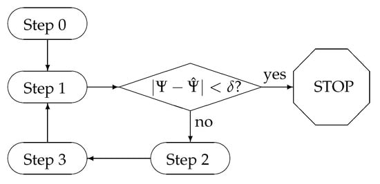
Figure 2.
Diagram of the algorithm for scenario selection.
- Step 0: initialization. Randomly select , and set the estimated social welfare as . Initialize the training dataset as empty.
- Step 1: social welfare calculation. Solve the GEP problem using Algorithm 1, and use its optimal solution and Equation (18) to calculate the actual social welfare for the set of high-quality scenarios .Checkpoint: The algorithm finishes if the error between actual and estimated social welfare is small enough and proceeds to Step 2 otherwise.
- Step 2: social welfare estimation. Add new results from Step 1 to the training dataset; obtain updated regression parameters for Model in Equation (20), then use the updated model to estimate social welfare values for the whole set of scenarios .
- Step 3: scenario selection. Update the set of high-quality scenarios by minimizing the Kantorovich distance from , , which was defined in Equation (19). Various heuristic algorithms, such as the golden section search method [49], can be used in this step. As proven by Dupačová et al. [17], the probabilities of high-quality scenarios are given by , where .
4. Case Study
We demonstrate the effectiveness of the proposed method in a case study, in which two transmission expansion plans are being evaluated for the U.S. Eastern and Western Interconnections. A total of one million scenarios were used to represent the uncertainty of the power system over the next 15 years, and the proposed algorithm was deployed to select ten high-quality scenarios for the two transmission plans.
4.1. Data and Computational Settings
We used the same dataset for the U.S. Eastern and Western Interconnections as used in [50] with some modifications. The dataset contained 169 buses, 730 transmission lines, 1640 existing generators, and 1568 candidate generators, representing the transmission infrastructures of the North American power grid. The locations of the 169 buses are shown in Figure 3. Demand for each year was divided into 19 load blocks. There were 60 generation technologies and fuel types, including coal, gas, oil, nuclear, hydro, geothermal, biomass, wind, and solar. Approximately 30% of existing generation capacity was renewable, and this ratio was required to increase by 1% each year, so that it would reach 45% by the end of year 15. One million demand and fuel cost elements of the scenarios were randomly generated with an average 1% annual growth rate for both. All algorithms were implemented in MATLAB [51], and to solve the models, we used MATLAB and the TOMLAB interface [52] to call CPLEX V.12 [53], used as the mixed integer linear programming solver.
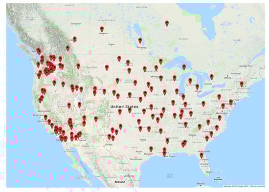
Figure 3.
Locations of the 169 buses.
4.2. Visualization of Power System Status
We designed a circular figure to visualize the status of the power system, as shown in Figure 4, which shows the status of the system in Year 0. All buses are represented by black dots and arranged in a circle according to their bus numbers from # 1 at the three o’clock position to # 169 in a clockwise direction. The blue lines inside this circle represent transmission lines that connect buses. Due to the circular arrangement of the dots, the lengths of the line segments in the figure are not proportional to the actual lengths of the transmission lines. The first layer outside the buses represents demand, with the lengths of the purple bars being proportional to the loads. Dark purple was used to indicate load shedding. The second layer represents generation capacity, with the lengths of the green bars being proportional to the generation capacity. Renewable and nonrenewable generation capacities are differentiated with light green and dark green colors, respectively. The third layer represents fuel costs, with the lengths of the orange bars being proportional to the average fuel cost for the generators at the associated buses. At the price of distorted geographical locations of the buses, this figure presents all three elements (demand, generation, and fuel cost) of scenarios considered in this study, allowing the decision maker to have an overview of the system status at once.
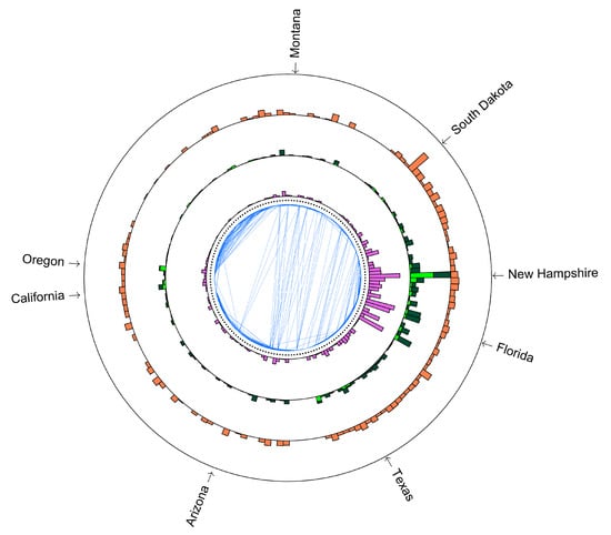
Figure 4.
Status of power system in Year 0. The inner circle represents the transmission network, and the outer layers with purple, green, and orange bars represent demand, generation capacity, and fuel cost, respectively. Renewable and nonrenewable generation capacities are differentiated with light green and dark green colors, respectively.
4.3. Validation of the Algorithm for Social Welfare Estimation
The algorithm for social welfare estimation from Section 3.2 was used in Step 2 of the algorithm for high-quality scenario selection. It took approximately 10 min to calculate the actual social welfare for one scenario. Using a termination criterion as for the training scenarios, the algorithm finished after calculating the actual social welfare for 50 scenarios (in approximately 8 h), which would have taken 19 years for the whole set of one million scenarios. To validate the quality of social welfare estimation, we calculated the actual social welfare for 100 random scenarios that were not used in the training set using Algorithm 1. Figure 5 compares the estimated and actual social welfare of these 100 scenarios, and the minimum, mean, and maximum of were 0.00%, 0.35%, and 0.95%, respectively, for these 100 scenarios.
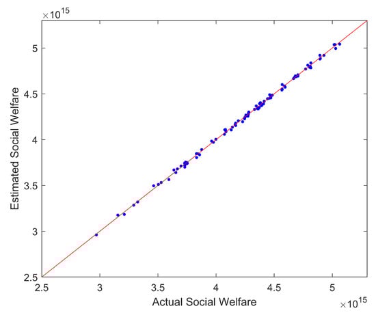
Figure 5.
The performance of the social welfare estimation model on 100 validation scenarios.
4.4. Scenario Selection for Two Transmission Plans
We demonstrate the effectiveness of the scenario selection algorithm in Section 3.3 using two transmission plans.
- Transmission Plan 1: existing transmission capacity will stay constant for the next 15 years without any expansion.
- Transmission Plan 2: the capacities of 26 congested lines will be doubled in Year 5, and another 27 congested lines will be doubled in Year 10.
Ten high-quality scenarios were selected for each transmission plan, and two of them are shown in Figure 6. Notice that the ten high-quality scenarios may be different for different plans, because power network topologies change under different plans. These figures illustrate how the power system would evolve in both the temporal and spatial dimensions with different transmission capacities under different scenarios. Although the selected scenarios demonstrated temporal and spatial correlations, it was not straightforward to interpret their social welfare implications, which demonstrated the need for the proposed algorithms for selecting high-quality scenarios.
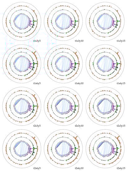
Figure 6.
High-quality scenarios for Transmission Plans 1 (t1) and 2 (t2), under Scenarios 3 (s3) and 6 (s6), and for Years 5 (y5), 10 (y10), and 15 (y15). Dark purple is used to indicate load shedding. The selected scenarios for two different plans are different because their power system structures are different. Hence, the iterative approach results in different high-quality scenarios for two different plans.
As a comparison with the proposed algorithm, we also used three other approaches to select ten scenarios for the two transmission plans:
- Random selection: ten scenarios were randomly selected from the whole set of one million scenarios.
- K-means: ten scenarios were selected using the K-means method [21] based on demand and fuel cost information of the whole set of one million scenarios.
- K-medoids: ten scenarios were selected using the K-medoids method [54] based on demand and fuel cost information of the whole set of one million scenarios.
Results from these methods are summarized in Table 4 and Table 5, in which the ten selected scenarios from each method are sorted in ascending order of social welfare and listed in the same ten rows (e.g., the row for Scenario 1 shows four different worst case scenarios selected using the four methods). Computationally, the proposed approach took approximately 8 h, whereas the other methods only took seconds.
Table 4.
Social welfare (, in $) and probability () of 10 selected scenarios and the Kantorovich distance ( in $) for Transmission Plan 1. The 10 selected scenarios for different approaches may be different.
Table 5.
Social welfare (, in $) and probability () of 10 selected scenarios and the Kantorovich distance ( in $) for Transmission Plan 2. The 10 selected scenarios for different approaches may be different.
4.5. Cost Benefit Analysis of Transmission Expansion
The analysis from Section 4.4 enables cost benefit analysis of Transmission Plan 2. As shown in Table 6, the difference between average social welfare across the whole set of one million scenarios for the two transmission plans was $5.23 trillion, which revealed the social benefit of Transmission Plan 2 throughout the 15-year horizon. The proposed approach estimated this difference as $4.99 trillion using the 10 high-quality scenarios. In comparison, the K-means approach over-estimated this value as $7.21 trillion; K-medoids under-estimated it as $2.16 trillion; and the random selection approach estimated this value to be negligible. These results suggested that the proposed approach was able to estimate the social benefit of transmission plans reasonably accurately, which also allowed it to be potentially integrated into the iterative stochastic TEP model proposed in Figure 1.
Table 6.
Average social welfare (in $) for the two transmission plans estimated using different methods.
5. Conclusions
The main contributions of this paper included a scenario selection method for iterative transmission planning, which had three salient features: (1) correlations between generation capacity and demand, fuel cost, and transmission capacity were explicitly captured; (2) high-quality scenarios were selected to minimize the Kantorovich distance of social welfare distributions between the selected and the whole set of scenarios; and (3) the set of high-quality scenarios was specific for each transmission plan, which enabled this approach to interact iteratively with a stochastic TEP model.
A case study was conducted to demonstrate the proposed approach, in which a 169-bus network was used to represent the U.S. Eastern and Western Interconnections. When compared with three other methods for scenario selection, our algorithm was found to provide a more accurate estimation of the economic value of transmission plans.
The proposed approach was not without its limitations and caveats. For example, the GEP model was a simplified estimation of the actual decision-making process, which involved far more realistic and complex constraints such as multiple decision makers and risk hedging constraints. We also acknowledge that there are numerous other sources of uncertainty in realistic transmission planning projects, which were not explicitly taken into consideration in the proposed approach, such as investment cost, growth rate of distributed energy resources, renewable energy production, energy policies, etc. Besides Kantorovich distance, other probabilistic distances could also be used as the selection criterion for high-quality scenarios. Moreover, the social welfare evaluation could be extended to include environmental and reliability benefits of the power system. Co-optimization of GEP and TEP is another potential topic for future research.
Author Contributions
F.A., L.W., and J.M. conceived the study. F.A. implemented the computational experiments. F.A. and L.W. wrote the paper. All authors read and agreed to the published version of the manuscript.
Funding
This work was supported by the Power Systems Engineering Research Center under the research project M-37.
Conflicts of Interest
The authors declare no conflict of interest.
References
- Hemmati, R.; Hooshmand, R.A.; Khodabakhshian, A. State-of-the-art of transmission expansion planning: Comprehensive review. Renew. Sustain. Energy Rev. 2013, 23, 312–319. [Google Scholar] [CrossRef]
- Lumbreras, S.; Ramos, A. The new challenges to transmission expansion planning. Survey of recent practice and literature review. Electr. Power Syst. Res. 2016, 134, 19–29. [Google Scholar] [CrossRef]
- Silva, I.d.J.; Rider, M.J.; Romero, R.; Murari, C.A. Transmission network expansion planning considering uncertainty in demand. IEEE Trans. Power Syst. 2006, 21, 1565–1573. [Google Scholar] [CrossRef]
- Qiu, J.; Zhao, J.; Wang, D. Flexible multi-objective transmission expansion planning with adjustable risk aversion. Energies 2017, 10, 1036. [Google Scholar] [CrossRef]
- Dehghan, S.; Kazemi, A.; Amjady, N. Multi-objective robust transmission expansion planning using information-gap decision theory and augmented ϵ-constraint method. IET Gener. Transm. Distrib. 2014, 8, 828–840. [Google Scholar] [CrossRef]
- Chen, B.; Wang, J.; Wang, L.; He, Y.; Wang, Z. Robust optimization for transmission expansion planning: Minimax cost vs. minimax regret. IEEE Trans. Power Syst. 2014, 29, 3069–3077. [Google Scholar] [CrossRef]
- Chen, B.; Wang, L. Robust transmission planning under uncertain generation investment and retirement. IEEE Trans. Power Syst. 2016, 31, 5144–5152. [Google Scholar] [CrossRef]
- Dehghan, S.; Amjady, N. Robust transmission and energy storage expansion planning in wind farm-integrated power systems considering transmission switching. IEEE Trans. Sustain. Energy 2016, 7, 765–774. [Google Scholar] [CrossRef]
- Dehghan, S.; Amjady, N.; Conejo, A.J. Adaptive robust transmission expansion planning using linear decision rules. IEEE Trans. Power Syst. 2017, 32, 4024–4034. [Google Scholar] [CrossRef]
- Liang, Z.; Chen, H.; Wang, X.; Ibn Idris, I.; Tan, B.; Zhang, C. An extreme scenario method for robust transmission expansion planning with wind power uncertainty. Energies 2018, 11, 2116. [Google Scholar] [CrossRef]
- López, J.A.; Ponnambalam, K.; Quintana, V.H. Generation and transmission expansion under risk using stochastic programming. IEEE Trans. Power Syst. 2007, 22, 1369–1378. [Google Scholar] [CrossRef]
- Bagheri, A.; Wang, J.; Zhao, C. Data-driven stochastic transmission expansion planning. IEEE Trans. Power Syst. 2017, 32, 3461–3470. [Google Scholar] [CrossRef]
- Liu, Y.; Sioshansi, R.; Conejo, A.J. Multistage stochastic investment planning with multiscale representation of uncertainties and decisions. IEEE Trans. Power Syst. 2018, 33, 781–791. [Google Scholar] [CrossRef]
- Park, H.; Baldick, R.; Morton, D.P. A stochastic transmission planning model with dependent load and wind forecasts. IEEE Trans. Power Syst. 2015, 30, 3003–3011. [Google Scholar] [CrossRef]
- Munoz, F.D.; Hobbs, B.F.; Ho, J.L.; Kasina, S. An engineering-economic approach to transmission planning under market and regulatory uncertainties: WECC case study. IEEE Trans. Power Syst. 2013, 29, 307–317. [Google Scholar] [CrossRef]
- Kim, W.W.; Park, J.K.; Yoon, Y.T.; Kim, M.K. Transmission expansion planning under uncertainty for investment options with various lead-times. Energies 2018, 11, 2429. [Google Scholar] [CrossRef]
- Dupačová, J.; Gröwe-Kuska, N.; Römisch, W. Scenario reduction in stochastic programming. Math. Program. 2003, 95, 493–511. [Google Scholar] [CrossRef]
- Gil, E.; Aravena, I.; Cárdenas, R. Generation capacity expansion planning under hydro uncertainty using stochastic mixed integer programming and scenario reduction. IEEE Trans. Power Syst. 2015, 30, 1838–1847. [Google Scholar] [CrossRef]
- Du, E.; Zhang, N.; Kang, C.; Bai, J.; Cheng, L.; Ding, Y. Impact of wind power scenario reduction techniques on stochastic unit commitment. In Proceedings of the 2016 Second International Symposium on Stochastic Models in Reliability Engineering, Life Science and Operations Management (SMRLO), Beer-Sheva, Israel, 15–18 February 2016; pp. 202–210. [Google Scholar]
- Feng, Y.; Ryan, S.M. Solution sensitivity-based scenario reduction for stochastic unit commitment. Comput. Manag. Sci. 2016, 13, 29–62. [Google Scholar] [CrossRef]
- Lin, C.; Fang, C.; Chen, Y.; Liu, S.; Bie, Z. Scenario generation and reduction methods for power flow examination of transmission expansion planning. In Proceedings of the 2017 IEEE 7th International Conference on Power and Energy Systems (ICPES), Toronto, ON, Canada, 1–3 November 2017; pp. 90–95. [Google Scholar]
- Hinojosa, V.; Gil, E.; Calle, I. A stochastic generation capacity expansion planning methodology using linear distribution factors and hourly load modeling. In Proceedings of the 2018 IEEE International Conference on Probabilistic Methods Applied to Power Systems (PMAPS), Boise, ID, USA, 24–28 June 2018; pp. 1–6. [Google Scholar]
- Hinojosa, V.; Velásquez, J. Stochastic security-constrained generation expansion planning based on linear distribution factors. Electr. Power Syst. Res. 2016, 140, 139–146. [Google Scholar] [CrossRef]
- Pineda, S.; Morales, J.M. Chronological time-period clustering for optimal capacity expansion planning with storage. IEEE Trans. Power Syst. 2018, 33, 7162–7170. [Google Scholar] [CrossRef]
- Park, S.; Xu, Q.; Hobbs, B. Comparing Scenario Reduction Methods for Stochastic Transmission Planning. IET Gener. Transm. Distrib. 2019, 13, 1005–1013. [Google Scholar] [CrossRef]
- Papavasiliou, A.; Oren, S.S. Multiarea stochastic unit commitment for high wind penetration in a transmission constrained network. Oper. Res. 2013, 61, 578–592. [Google Scholar] [CrossRef]
- Dupačová, J.; Consigli, G.; Wallace, S.W. Scenarios for multistage stochastic programs. Ann. Oper. Res. 2000, 100, 25–53. [Google Scholar] [CrossRef]
- Growe-Kuska, N.; Heitsch, H.; Romisch, W. Scenario reduction and scenario tree construction for power management problems. In Proceedings of the 2003 IEEE Bologna Power Tech Conference Proceedings, Bologna, Italy, 23–26 June 2003; Volume 3, p. 7. [Google Scholar]
- Sun, M.; Cremer, J.; Strbac, G. A novel data-driven scenario generation framework for transmission expansion planning with high renewable energy penetration. Appl. Energy 2018, 228, 546–555. [Google Scholar] [CrossRef]
- Li, J.; Ye, L.; Zeng, Y.; Wei, H. A scenario-based robust transmission network expansion planning method for consideration of wind power uncertainties. CSEE J. Power Energy Syst. 2016, 2, 11–18. [Google Scholar] [CrossRef]
- Ehsan, A.; Yang, Q.; Cheng, M. A scenario-based robust investment planning model for multi-type distributed generation under uncertainties. IET Gener. Transm. Distrib. 2018, 12, 4426–4434. [Google Scholar] [CrossRef]
- Sun, M.; Teng, F.; Konstantelos, I.; Strbac, G. An objective-based scenario selection method for transmission network expansion planning with multivariate stochasticity in load and renewable energy sources. Energy 2018, 145, 871–885. [Google Scholar] [CrossRef]
- Flamos, A. A sectoral micro-economic approach to scenario selection and development: The case of the Greek power sector. Energies 2016, 9, 77. [Google Scholar] [CrossRef]
- Wang, J.; Shahidehpour, M.; Li, Z.; Botterud, A. Strategic generation capacity expansion planning with incomplete information. IEEE Trans. Power Syst. 2009, 24, 1002–1010. [Google Scholar] [CrossRef]
- Zhou, Y.; Wang, L.; McCalley, J.D. Designing effective and efficient incentive policies for renewable energy in generation expansion planning. Appl. Energy 2011, 88, 2201–2209. [Google Scholar] [CrossRef]
- Palmintier, B.; Webster, M. Impact of unit commitment constraints on generation expansion planning with renewables. In Proceedings of the 2011 IEEE Power and Energy Society General Meeting, Detroit, MI, USA, 24–29 July 2011; pp. 1–7. [Google Scholar]
- Aghaei, J.; Akbari, M.A.; Roosta, A.; Baharvandi, A. Multiobjective generation expansion planning considering power system adequacy. Electr. Power Syst. Res. 2013, 102, 8–19. [Google Scholar] [CrossRef]
- Rashidaee, S.A.; Amraee, T.; Fotuhi-Firuzabad, M. A Linear Model for Dynamic Generation Expansion Planning Considering Loss of Load Probability. IEEE Trans. Power Syst. 2018, 33, 6924–6934. [Google Scholar] [CrossRef]
- De La Torre, S.; Conejo, A.J.; Contreras, J. Transmission expansion planning in electricity markets. IEEE Trans. Power Syst. 2008, 23, 238–248. [Google Scholar] [CrossRef]
- Shrestha, G.; Fonseka, P. Congestion-driven transmission expansion in competitive power markets. IEEE Trans. Power Syst. 2004, 19, 1658–1665. [Google Scholar] [CrossRef]
- Garcés, L.P.; Conejo, A.J.; García-Bertrand, R.; Romero, R. A bilevel approach to transmission expansion planning within a market environment. IEEE Trans. Power Syst. 2009, 24, 1513–1522. [Google Scholar] [CrossRef]
- Sauma, E.E.; Oren, S.S. Economic criteria for planning transmission investment in restructured electricity markets. IEEE Trans. Power Syst. 2007, 22, 1394–1405. [Google Scholar] [CrossRef]
- Sauma, E.E.; Oren, S.S. Proactive planning and valuation of transmission investments in restructured electricity markets. J. Regul. Econom. 2006, 30, 358–387. [Google Scholar] [CrossRef]
- Jenabi, M.; Ghomi, S.M.T.F.; Smeers, Y. Bi-level game approaches for coordination of generation and transmission expansion planning within a market environment. IEEE Trans. Power Syst. 2013, 28, 2639–2650. [Google Scholar] [CrossRef]
- Hwang, Y.M.; Sim, I.; Sun, Y.G.; Lee, H.J.; Kim, J.Y. Game-Theory Modeling for Social Welfare Maximization in Smart Grids. Energies 2018, 11, 2315. [Google Scholar] [CrossRef]
- Kantorovich, L. On the transfer of masses, Dok 1. Akad. Nauk SSSR 1942, 37, 227–229. [Google Scholar]
- Bard, J.F.; Moore, J.T. A branch and bound algorithm for the bilevel programming problem. SIAM J. Sci. Stat. Comput. 1990, 11, 281–292. [Google Scholar] [CrossRef]
- Fortuny-Amat, J.; McCarl, B. A representation and economic interpretation of a two-level programming problem. J. Oper. Res. Soc. 1981, 32, 783–792. [Google Scholar] [CrossRef]
- Chang, Y.C. N-dimension golden section search: Its variants and limitations. In Proceedings of the 2009 2nd International Conference on Biomedical Engineering and Informatics, Tianjin, China, 17–19 October 2009; pp. 1–6. [Google Scholar]
- Figueroa-Acevedo, A.L. Opportunities and Benefits for Increasing Transmission Capacity between the US Eastern and Western Interconnections. Ph.D. Thesis, Iowa State University, Ames, IA, USA, 2017. [Google Scholar]
- The Mathworks, Inc. MATLAB version 9.4.0.813654 (R2018a); The Mathworks, Inc.: Natick, MA, USA, 2018. [Google Scholar]
- Holmström, K.; Göran, A.O.; Edvall, M.M. User’s guide for Tomlab/CPLEX v12. 1. Tomlab Optim. Retr. July 2009, 1, 2017. [Google Scholar]
- Cplex, I.I. V12. 1: User’s Manual for CPLEX. Int. Bus. Mach. Corp. 2009, 46, 157. [Google Scholar]
- Wang, Q.; Dong, W.; Yang, L. A wind power/photovoltaic typical scenario set generation algorithm based on Wasserstein distance metric and revised K-medoids cluster. Proc. CSEE 2015, 35, 2654–2661. [Google Scholar]


© 2020 by the authors. Licensee MDPI, Basel, Switzerland. This article is an open access article distributed under the terms and conditions of the Creative Commons Attribution (CC BY) license (http://creativecommons.org/licenses/by/4.0/).