1. Introduction
The National Center for Atmospheric Research (NCAR), in collaboration with Xcel Energy addressing users’ needs and requirements, has developed a comprehensive wind power forecasting system. The original forecasting system was designed for day-ahead forecasting to support power trading. The new augmented and enhanced forecasting system provides capabilities for short-term forecasting, including wind ramp detection, prediction of extreme events such as icing conditions that can significantly impact wind power production when wind resource is abundant, empirical wind-to-power conversion techniques, and uncertainty quantification in power forecasting. This system employs artificial intelligence methods [
1,
2,
3] to integrate disparate data sources with publicly available numerical weather prediction model outputs. The development of the new comprehensive forecasting system is motivated by risk reduction of wind power integration into a power grid and reduction of the levelized cost of wind power.
The wind power forecasting system provides essential information for effective integration of variable generation into the power grid and addresses requirements for both the effective maintenance of reliable electric grids and energy trading. The grid operators and energy traders require accurate wind power forecasts at time scales spanning a range from minutes to several days ahead. Since no single weather forecasting methodology can perform optimally across all these temporal scales, we have combined numerical weather predictions (NWPs) that provides skillful predictions at times beyond a few hours with specialized methods based on observations that can improve the very short-range forecasts.
To develop a decision support system for the effective integration of variable generations, we have leveraged proven forecasting methodologies for each temporal, as well as spatial, scale. Disparate sources of data, including power generation data, as well as local and regional weather observations, are combined using artificial intelligence methods with the information about physics and dynamics of the atmosphere to predict power output [
4,
5,
6,
7]. In addition, advance knowledge of extreme events, such as ice storms, can greatly aid system operations and methods, and tools for generating warnings of potential impacts of these processes on wind power generation are developed.
The schematic diagram of the comprehensive wind power forecasting system [
1,
2,
3] developed by NCAR is shown in
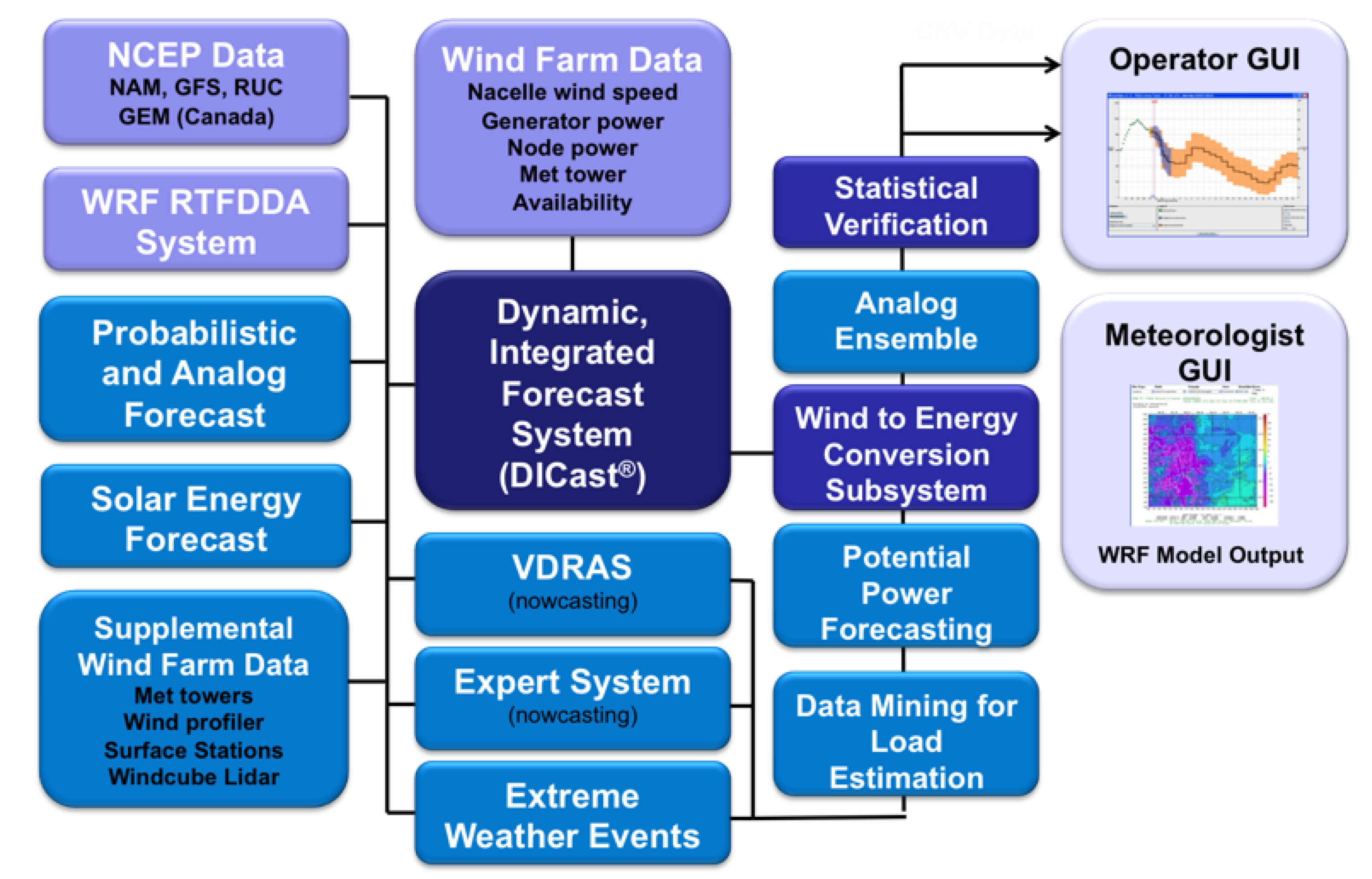
Figure 1. The central component of the system is the Dynamic Integrated foreCast System (DICast®). DICast is an advanced machine-learning module that has been under development at NCAR for over twenty years. It blends publicly available model output and high-resolution NWP models configured for Xcel Energy’s regions with weather observations form wind farms and routine meteorological surfaces and upper air observations. The wind farm data include wind speed measurements from Nacelle mounted anemometers. For an improved short-term forecast of wind ramps, we have also integrated the variational doppler radar analysis system (VDRAS) together with an observation-based expert system. An alternative for short-term forecasting is the regime-switching approach [
8,
9]. While the regime-switching approach has proven effective, our focus was on providing more accurate physical models for short-term forecasting in the summertime when convective storm outflows are responsible for numerous wind ramps throughout the areas served by Xcel Energy. By assimilating radar observations, VDRAS is able to provide accurate short-term forecasts not only of frontal passages when wind regimes switch but also storm outflows.
DICast provides deterministic wind speed point forecasts at the location of interest; however, energy traders and grid operators require power forecasts. We have developed an empirical power conversion algorithm and combined it with an analog ensemble (AnEn) approach to quantify the uncertainty of these predictions. Furthermore, we have developed an icing potential warning system.
This paper describes numerical weather prediction (NWP) applications in
Section 2, followed by statistical processing and power conversion in
Section 3 and probabilistic prediction in
Section 4.
Section 5 treats the short-term problem of forecasting ramps. The AI-based extreme weather prediction system is described in
Section 6.
Section 7 summarizes and provides some thoughts for future applications.
2. Numerical Weather Prediction
In addition to publicly available NWP model output in the wind forecasting system, we use a limited area, high-resolution NWP system based on the Weather Research and Forecasting (WRF) model, specifically configured for the areas of interest. The WRF model is a community mesoscale NWP model designed for both operational forecasting and atmospheric research needs for a range of applications [
10]. It is maintained by NCAR and continually enhanced by university partners and a wider research community with over 20,000 users across the world. NOAA uses WRF as the basis of their operational 3-km high-resolution rapid refresh system, which runs hourly over the contiguous United States [
11].
WRF includes many options for approaches to the physics, uses state-of-the-science numerical procedures, and can be configured to run over the desired domains. The team carefully configured the combination of physics schemes to optimize the prediction of boundary layer wind speed using the Yonsei University (YSU) planetary boundary layer model, Monin-Obukhov surface layer scheme, Dudhia shortwave radiation model, rapid radiative transfer model (RRTM) for longwave radiation, Grell-Devenyi ensemble cumulus parameterization, Noah land surface model, and the Thompson microphysics parameterization.
WRF is initialized with boundary conditions from the U.S. National Centers for Environmental Prediction (NCEP) global forecasting system (GFS). To optimize the model for the site, local data are assimilated into the model. NCAR applies a WRF-based real-time four-dimensional data assimilation (RTFDDA) system for wind power prediction, which is based on Newtonian relaxation [
12] and adds forcing terms in the equations for momentum, temperature, and moisture. These terms “nudge” the model solution to agree better with the local observations. This nudging approach forces the equations toward a state that represents the current state of the observed atmosphere subjects to maintaining a smooth solution to the equations of fluid motion. NCAR assimilates standard meteorological observations plus the local wind farm observations.
One of the important considerations when setting up an NWP system for wind power forecasting is to collect and assimilate observations obtained at the wind farms. All wind turbines are equipped with Nacelle anemometers, which measure wind speed at a high temporal frequency. Although the wind measurements from individual turbines may present systematic errors caused by the disturbances generated by the turbine blades, aggregating clusters of observations from these Nacelle anemometers have been shown to be well-correlated with inflow wind speeds [
13,
14] and, therefore, well-represent wind intensity for a mesoscale NWP model [
15].
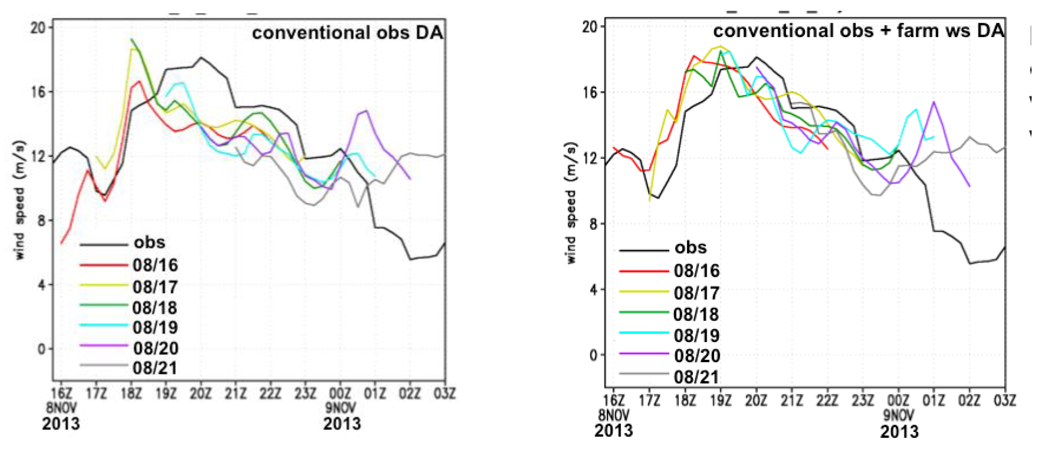
Figure 2 compares the model forecast with and without assimilation of the wind turbine hub-height (80 m) wind speed measurement for November 8-9, 2013. Assimilating the wind turbine hub-height wind significantly improved short-term wind predictions for this case, as well as others [
15].
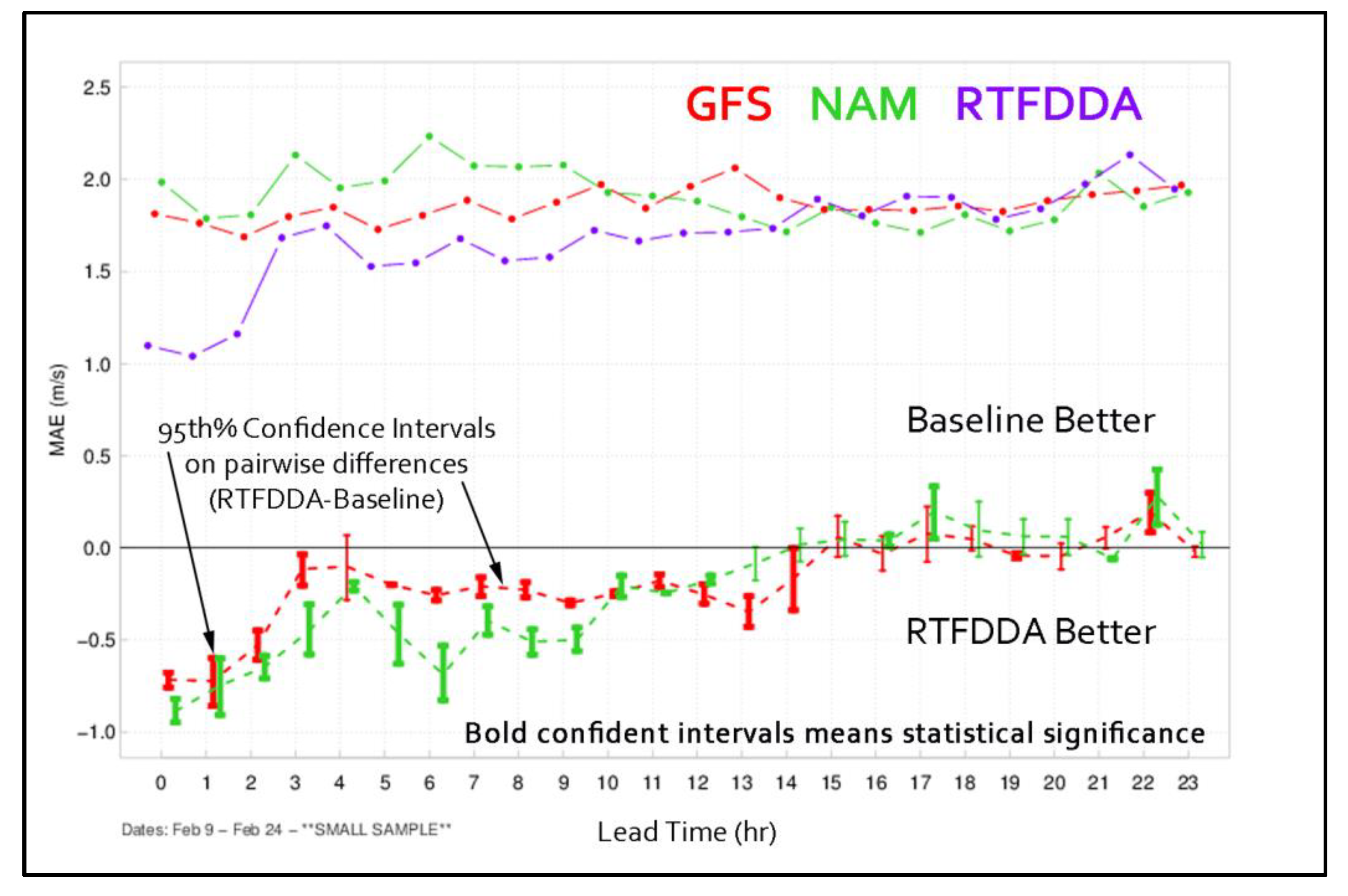
The performance of WRF RTFDDA was compared to that of the global forecast system (GFS) and North American model (NAM) to determine whether WRF RTFDDA significantly improved over the operational guidance provided by these National Center for Environmental Prediction (NCEP) models.
Figure 3 provides the mean absolute error (MAE) with an increasing forecast horizon (lead time). The scores were aggregated over a two-week period from 9–24 February, 2014.
The pairwise differences between WRF RTFDDA and the operational benchmarks are provided at the bottom of
Figure 3. The 95th percentile confidence intervals applied to the difference curves indicate that the improvements are statistically significant for most of those hours. During this period, WRF RTFDDA (purple) outperformed both GFS (red) and NAM (green) out to 15 and 14 h, respectively, with the differences on the order of 0.75 ms
−1 in the first few hours. After 15 h, the MAE values cluster around 1.8 ms
−1 for all the three models. These results suggest WRF RTFDDA provides value beyond the coarser operational models out to 15 h.
3. Statistical Postprocessing
The NWP model forecasts, including both the customized WRF RTFDDA runs described above and output freely available from the national centers, can be combined and optimized to improve upon the best forecasts. NCAR uses the Dynamic Integrated Forecast System (DICast®) to seamlessly blend and optimize the wind speed forecasts [
16]. DICast has been employed in numerous operational forecast systems developed by NCAR for forecasting temperature, humidity, precipitation, irradiance, and other meteorological variables for applications, including short- and medium-range weather forecasts, surface transportation, energy applications, and other decision support applications. The AI system takes a two-step process: it first applies dynamic model output statistics, which uses multilinear regression to remove bias from each model individually. It then generates a consensus forecast by using optimization methods to derive weighting coefficients to blend the models [
1,
2,
3,
16]. DICast thus constantly improves the forecast by learning from past errors based on comparisons of recent forecasts with observations. An advantage of DICast is that it best optimizes forecasts with a mere 90 days of data and can even produce skilled forecasts with as little as 30 days of training.
The wind power forecasting system ingests real-time observations of both hub-height wind speed and power from most of the wind turbines. The system utilizes the Nacelle hub-height wind speeds and turbine power from each turbine, because it correlates best with the turbine power.
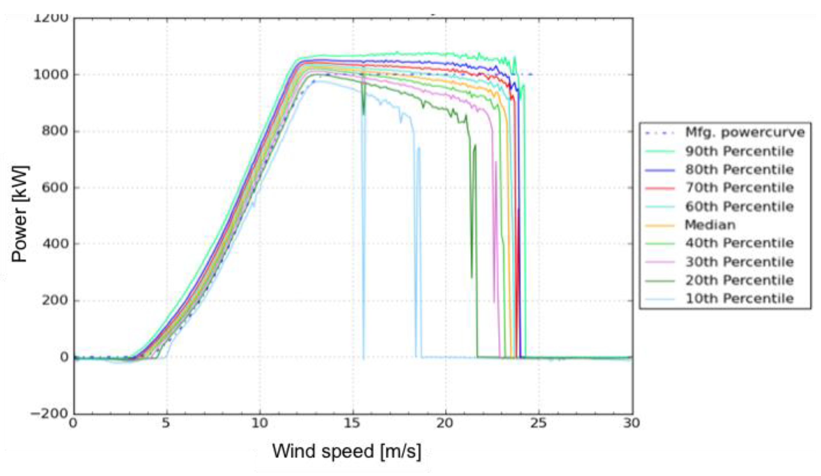
Although the weather variables are what are typically produced by DICast, the utility requires an estimate of power production. Manufacturers provide power curves that relate wind speed to power; however, the actual power often deviates substantially due to site-specific influences such as elevation, terrain, and land cover. Thus, NCAR’s wind power forecasting system takes an empirical approach to power conversion. A dataset of historical fit Nacelle wind speeds (15 minute averages) and coincident power production for each type of turbine at each wind farm is data mined using the regression tree, Cubist (RuleQuest Research.
https://www.rulequest.com/cubist-info.html); this allows identification of similar conditions during real-time operations in order to identify the correct portion of the empirical power curve to use for the conversion. The empirical power conversion model is based on the hierarchical regression tree model similar to the one described in the book Data Science for Wind Energy [
9]. In the enhanced system, the historical data were divided into quantiles, and only the inner quantiles (such as the inner 50th percentile) were used for the training. Thus, we can avoid training to extreme events, including, curtailments and high-speed cutouts. The parameters that dictate the extreme quantiles to be removed are configurable by the user for each connection node. The system forecasts power for each wind turbine. Those forecasts are then rolled up (summed) to produce predictions for the connection node (typically, a single wind farm). If information is available regarding special conditions, such as planned outages (such as for maintenance), that is considered in finalizing the forecast.
Figure 4 is an example of the data-mined power curves for each decile. Thus, as seen by observing the spread of the percentile curves, the middle 50% of the power values could be considered as more representative of the power curve. This is a quality control approach that provides site-specific empirical power conversion that better represents the actual relationship between observed wind speed and produced power than the manufacturer’s power curve.
Automatic verification is used to monitor the performance of the system by tracking the normalized mean absolute error (NMAE). The NMAE is obtained by normalizing the mean absolute error by the connection node maximum capacity to produce a percent error. The system runs at about 10% NMAE.
4. Probabilistic Prediction
Utilities such as Xcel Energy require probabilistic information to quantify the uncertainty in the forecasts. The traditional approach in NWP has been to run a set of model forecasts to form an ensemble that represents runs with different initial conditions, boundary conditions, physics packages, etc. Here, we employ a newer and more efficient AI approach of identifying analogs within a historical dataset, including past deterministic forecasts and observations of the quantity to be predicted. Specifically, for a given forecast lead time and location, we compare the current DICast prediction with past predictions to determine the closest analogs. We then select the past wind speed observations that correspond to those analog forecasts. Those observations form the AnEn prediction for that lead time and location. This procedure is repeated for each desired lead time and location. Probabilistic forecasting, including an example of wind speed forecasting, was reviewed by Gneiting and Katzfuss [
17]. They formalized the calibration of predictive distributions and assessed their sharpness by defining scoring rules, including the logarithmic score and the continuous ranked probability score. The AnEn approach has been shown to maintain or improve the accuracy of the deterministic prediction that is used to build it, as well as providing an accurate and reliable probabilistic forecast based on the metrics defined by Gneiting and Katzfuss [
18,
19]. While for short-term forecasting an effective forecasting approach is based on the calibrated regime-switching method [
8,
20], the AnEn was selected because it combines the NWP model output with observations, and it is therefore applicable to forecasting at any timeframe.
Here, we have applied the AnEn to generate wind forecasts at over 67 wind farms located in Colorado and Wyoming managed by Xcel Energy. Wind observations were available for a 223-day period (from 19 October 2013 to 11 June 2014) together with DICast daily forecasts of wind speed, wind direction at the hub-height, and sea level pressure starting at 12 UTC to generate 1–73 h predictions. The last 35 days of this period were used to test the AnEn performance and to carry out a comparison with DICast wind speed predictions. The remaining portion of the dataset was used for training. The set of optimal weights is defined by choosing, independently for each station, the combination that minimizes the continuous ranked probability score (CRPS) over the training period, defined as:
where
is the total number of observations,
is the cumulative distribution function (CDF) of the forecast variable being less or equal to
at the space-time location of observation
is the CDF of the observation (a Heaviside function). CRPS is a negatively oriented metric (i.e., lower scores are better) with a perfect score of 0.
We determine optimal weights in the analog matching metric following [
21] for each of the four analog predictors.
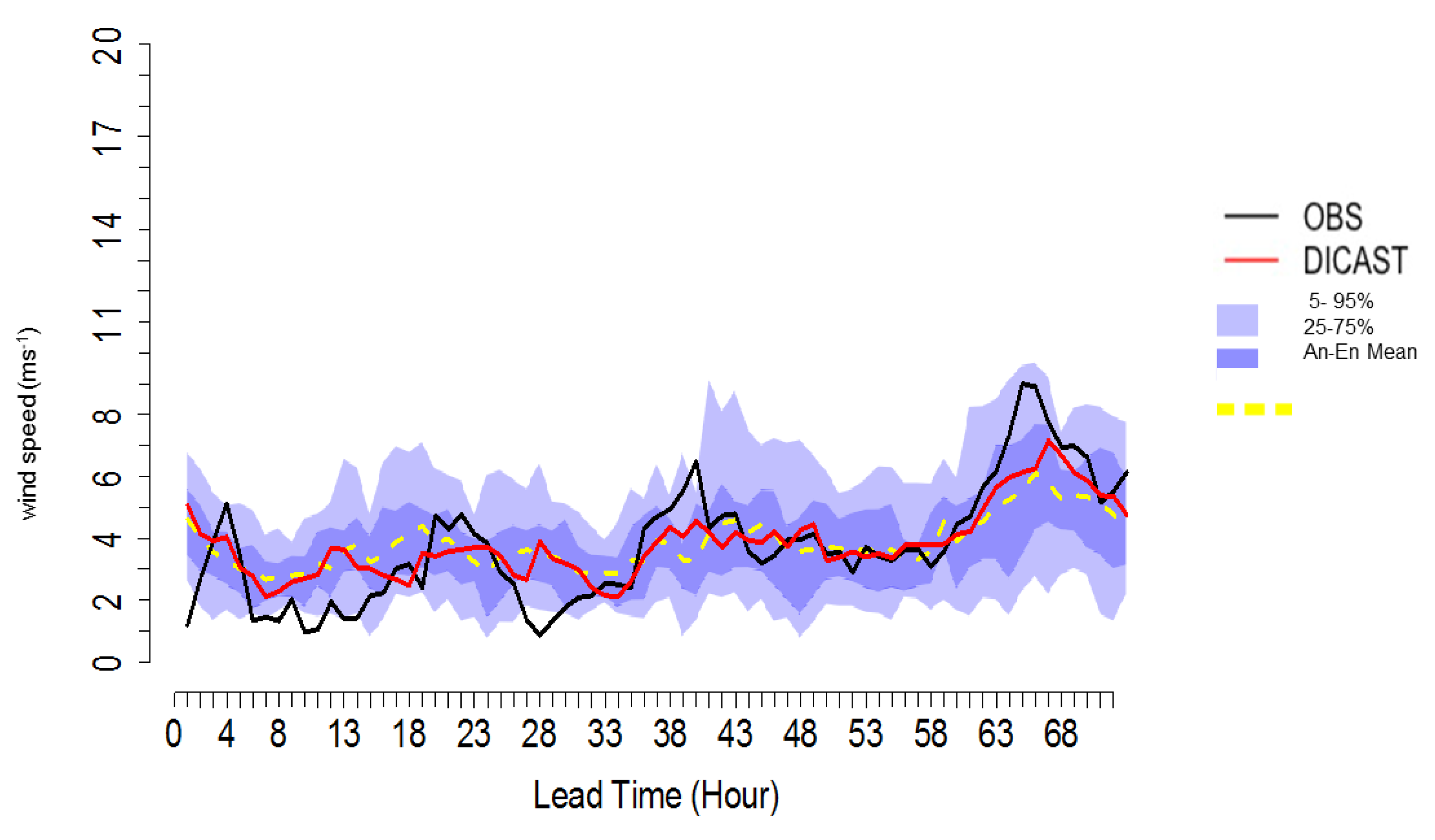
Figure 5 provides an example of the AnEn forecasts, where AnEn means are compared with wind speed predictions obtained from DICast. Thus, the AnEn maintains the accuracy of the DICast deterministic prediction while additionally providing uncertainty quantification. This example also shows the usefulness of a probabilistic prediction; although the deterministic predictions underestimate some of the highest speeds (e.g., lead time hour 65), the ensemble distribution (represented by the shading) does provide for the high observed value a certain level of likelihood.
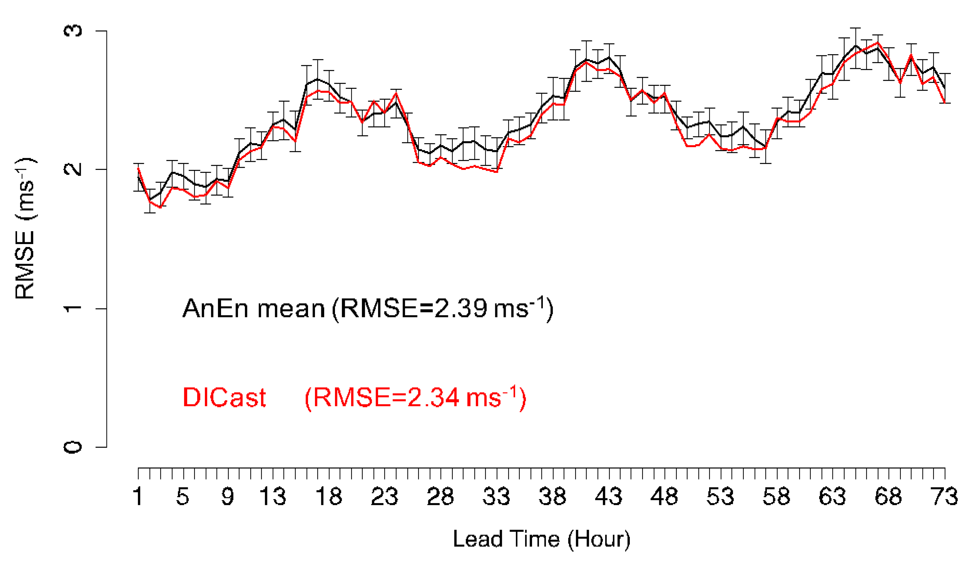
In
Figure 6, the AnEn mean is compared to DICast in terms of the root mean square error (RMSE) computed from forecast hour 1 to 73 and over all the available stations. The bootstrap confidence intervals suggest that there is no statistically significant difference between the AnEn and DICast performances for these forecasts. Hence, the AnEn mean can maintain the same level of accuracy as DICast for the deterministic prediction.
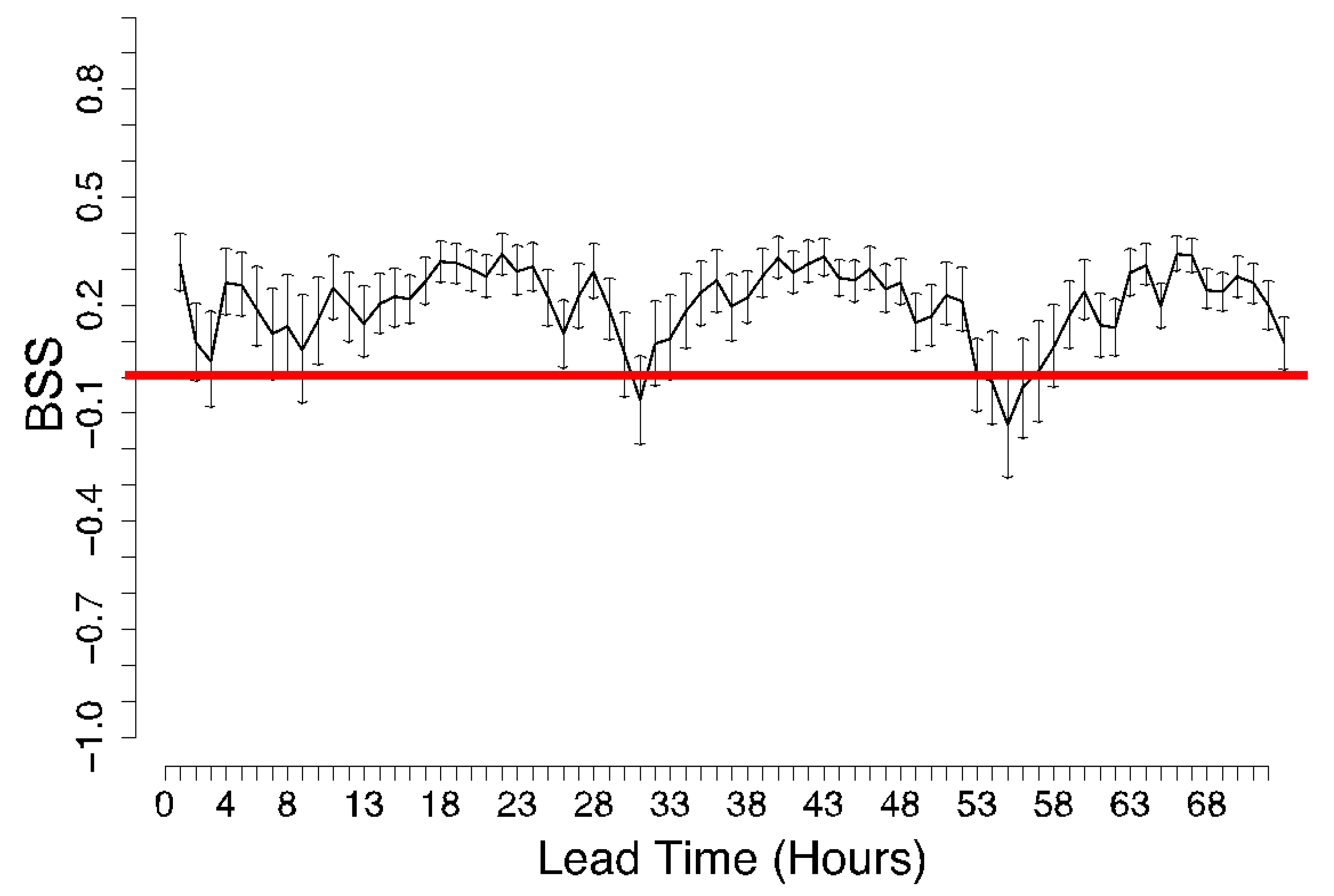
Figure 7 depicts the Brier skill score (BSS) [
16] of the AnEn computed over all the stations with DICast as a reference. An assessment of important probabilistic prediction attributes such as reliability and resolution can be performed by calculating the Brier score (BS) components. The Brier score is similar to the RMSE for a deterministic forecast. It is computed as:
where
is the total number of forecast/observation pairs,
is the forecasted probability of a categorical event (e.g., in this case, wind speed greater than 10 ms
−1), and
is the categorical observation (0 if the event does not occur and 1 if it does occur). A lower value of the Brier score indicates better performance, with 0 corresponding to a perfect forecast. Using the DICast forecast as a reference, the Brier skill score (BSS) is calculated as:
where
BSDICast is the
BS of DICast. In the case of DICast,
pn in (2) can only take 1 or 0 values, e.g., if the forecasted wind speed is greater or lower than 10 ms
−1, respectively. The
BSS represents the measure of the probabilistic forecast performance in comparison to the reference forecast and measures the ability of the model to issue a better probabilistic forecast than the reference. Positive (negative) values of BSS indicate better (worse) performances of AnEn than DICast.
Figure 7 indicates the benefit of using a probabilistic forecast system such as AnEn, rather than a deterministic one. Although the AnEn and DICast show a similar level of performance when compared as deterministic systems (
Figure 5), a probabilistic score such as the BSS indicates that AnEn improves upon DICast deterministic forecasts by about 20%–30% for most lead times.
5. Short-range Forecasting
Large variations in available wind power over a short time (~30 min), or ramps, represent a challenge for grid operators. The system should ideally predict the timing, magnitude, and duration of these ramps. The latency of availability of NWP model output combined with the inherent uncertainties in the timing of wind ramps makes the use of NWP for these short-range forecasts quite challenging. The best strategies for these nowcasts (0 to about 3 h ahead) rely on observations near the wind farm. NCAR evaluated two systems: an AI observation-based expert system that utilizes upstream observations and the variational doppler radar analysis system (VDRAS) [
22].
As described previously [
1], VDRAS is based on a numerical cloud scale model that produces high-resolution boundary-layer wind fields. The key to its success is in assimilating radar radial velocity data obtained from reflectivity measurements. The VDRAS system has proven useful for many applications, including at defense ranges, for homeland security applications, and internationally in support of the Olympics [
23]. VDRAS is run at about 1–4-km spatial resolution and is able to produce forecasts as frequently as every 10 minutes. It produces wind, thermodynamical, and microphysical analyses. VDRAS first assimilates data from various sources, including background weather data from the WRF RTFDDA model forecasts, surface network observations, and radar data. For efficient, operationally feasible simulation runs, the VDRAS domain must be limited in size yet big enough to include the nearby doppler radar sites.
VDRAS simulations are used for short-range forecasting. These simulations enable distinguishing large-scale features such as cold fronts from thunderstorm gust fronts or low-level jets, as well as other weather phenomena characterized by strong wind gradients. The cloud-scale VDRAS model provides high-resolution forecasts resolving identified features and their location with up to two-hour lead times. While VDRAS-based wind nowcasts have shown some promise in case studies and real-time demonstrations, considerable effort is being undertaken to tackle the challenging problem of wind ramp prediction.
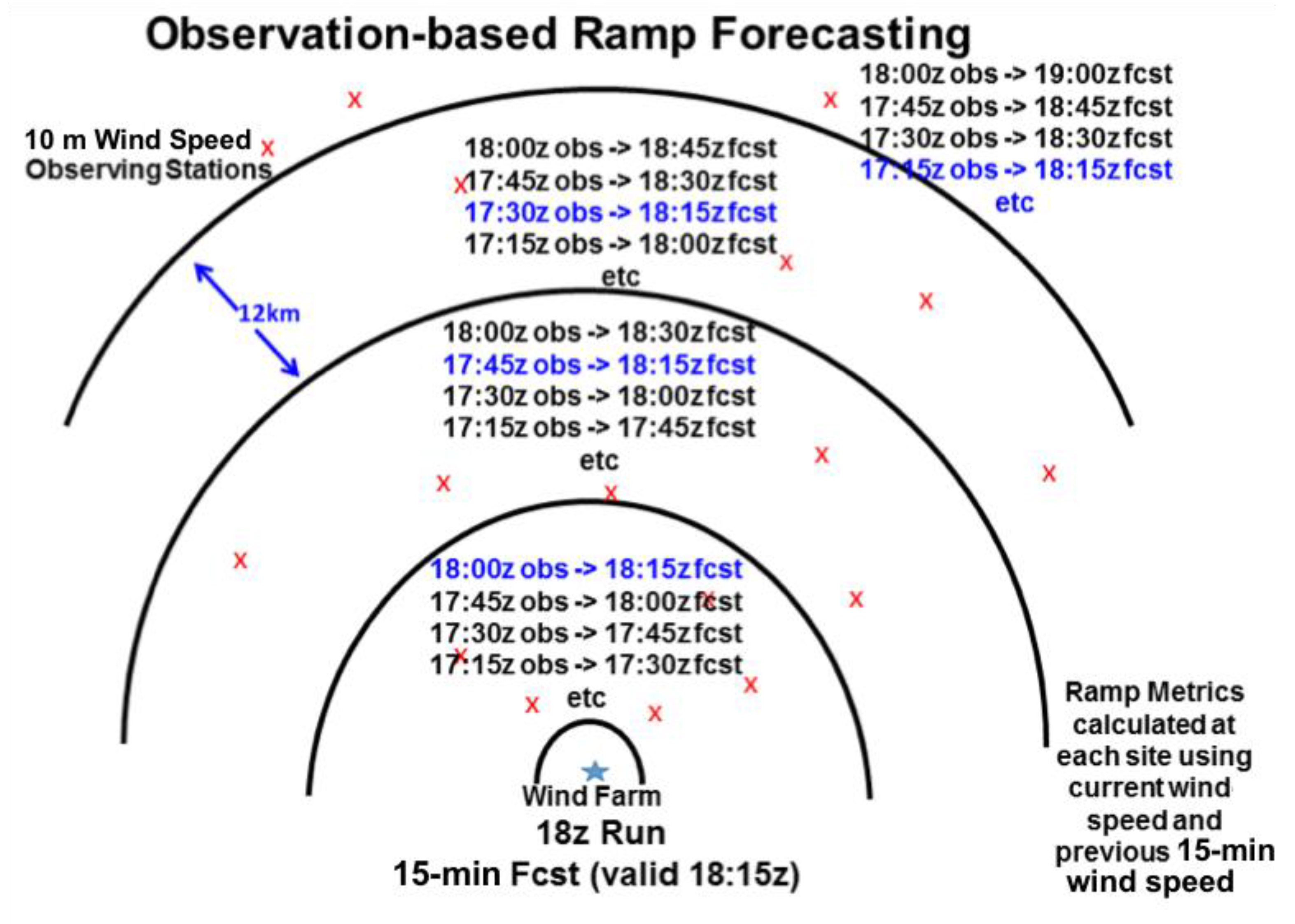
NCAR’s short-range expert forecasting system leverages publicly available surface observations of 10-m wind speeds upstream of the wind farms. The expert system is designed to predict ramps related to changes in power at a wind farm in 15-min intervals with two hours’ lead time. Observing sites are grouped in up to twelve concentric rings approximately 12-km-wide centered on a wind farm (see
Figure 8). The system detects wind ramp signatures upstream from a wind farm by calculating a ramp metric based on all the observations in a group. For a given forecast lead time, an average ramp metric is computed based on all the relevant group ramp metrics.
To best predict ramps, the VDRAS output is blended with the expert system results. Each of these two forecasting approaches is assigned a confidence level. The blended output describes the change in power production expected at each farm that is used to define a ramp metric. For a given lead time, the change in power production at each farm is calculated by multiplying the farm capacity by the ramp metric computed from the blended short-range system. The regional ramp forecast is created by aggregating the predicted changes in power across all the wind farms within the region, providing the utility information about the aggregate impact of the wind event.
6. Predicting Extreme Weather
The effects of ice accretion on wind turbines present a major challenge to operators, because the accreted ice will result in less power output than for a clean turbine blade. This needs to be accounted for to produce an accurate power forecast. Thus, a subsystem is included in the wind power forecast system for identifying not only icing conditions but also possible extreme temperatures and high wind speeds. The latter two hazards may also curtail power production due to operational decisions to shut down turbines. This subsystem, the extreme weather system or ExWx, combines wind and weather forecasts from the DICast forecasting system with the WRF RTFDDA model output and simple rules based on the forecaster’s experience. The result is an AI expert system that is highly configurable to suit a wide range of operator needs.
Development of the extreme weather system was modeled extensively on expert systems currently used in forecasting and diagnosing icing conditions for aircraft [
24,
25]. These algorithms employ adaptations of fuzzy logic theory and membership functions to combine datasets from multiple sources and to diagnose the current state or predict the future state. In ExWx, these same concepts are applied to forecasts of icing conditions, high wind speed events, and low and high temperature extremes.
6.1. Input Forecasts
Optimal configuration of the ExWx includes high-resolution NWP model (WRF RTFDDA—
Section 2) model output with output from the DICast forecasting system (
Section 3). The WRF RTFDDA model output provides the ExWx with forecasts of temperature, liquid cloud droplets, and liquid rain drops at a 3-km horizontal grid spacing with variable vertical grid spacing that is higher in the lower levels of the atmosphere. Forecasts of liquid water (cloud and rain) content from WRF RTFDDA are generated by the Thompson microphysics parameterization [
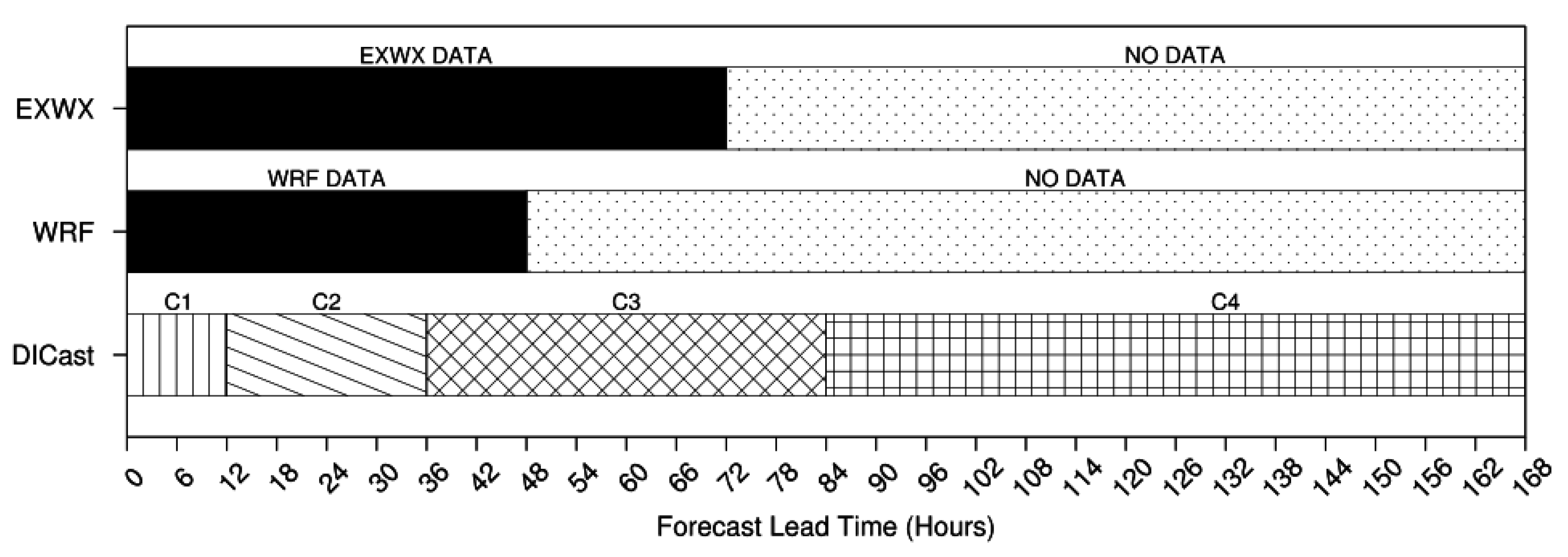
26] implemented in the WRF simulations. Forecasts from the WRF RTFDDA system are available with lead times ranging from 0–48 h.
DICast forecasts are available at select points within the operating region of a particular wind farm. These points must be chosen a priori and, in the current system, were selected at a horizontal spacing approximately equivalent to the coarsest horizontal grid spacing of all of the models used by DICast. At each of these points, DICast provides a forecast of icing conditions at the surface through a variable known as the conditional probability of icing (CPOI). The calculation of CPOI in DICast uses explicit model forecasts of surface precipitation types that could lead to turbine icing, as well as temperature and wet-bulb temperature, to determine the final likelihood of icing. The ExWx system produces forecasts for lead times 0–72 h (
Figure 9).
6.2. Forecasts
The WRF and DICast model outputs do not provide the same information for icing forecasts. To utilize both forecasts, an icing potential is computed. For the WRF output, this is simply at each grid box, while for DICast, it is for each available location nearby. The icing potential is an uncalibrated likelihood that icing conditions will be possible given the forecast input data. This unitless value ranges from 0 to 1, with 1 being the certainty of icing conditions. The ExWx system is configured based on testing and evaluation of the input datasets currently in use.
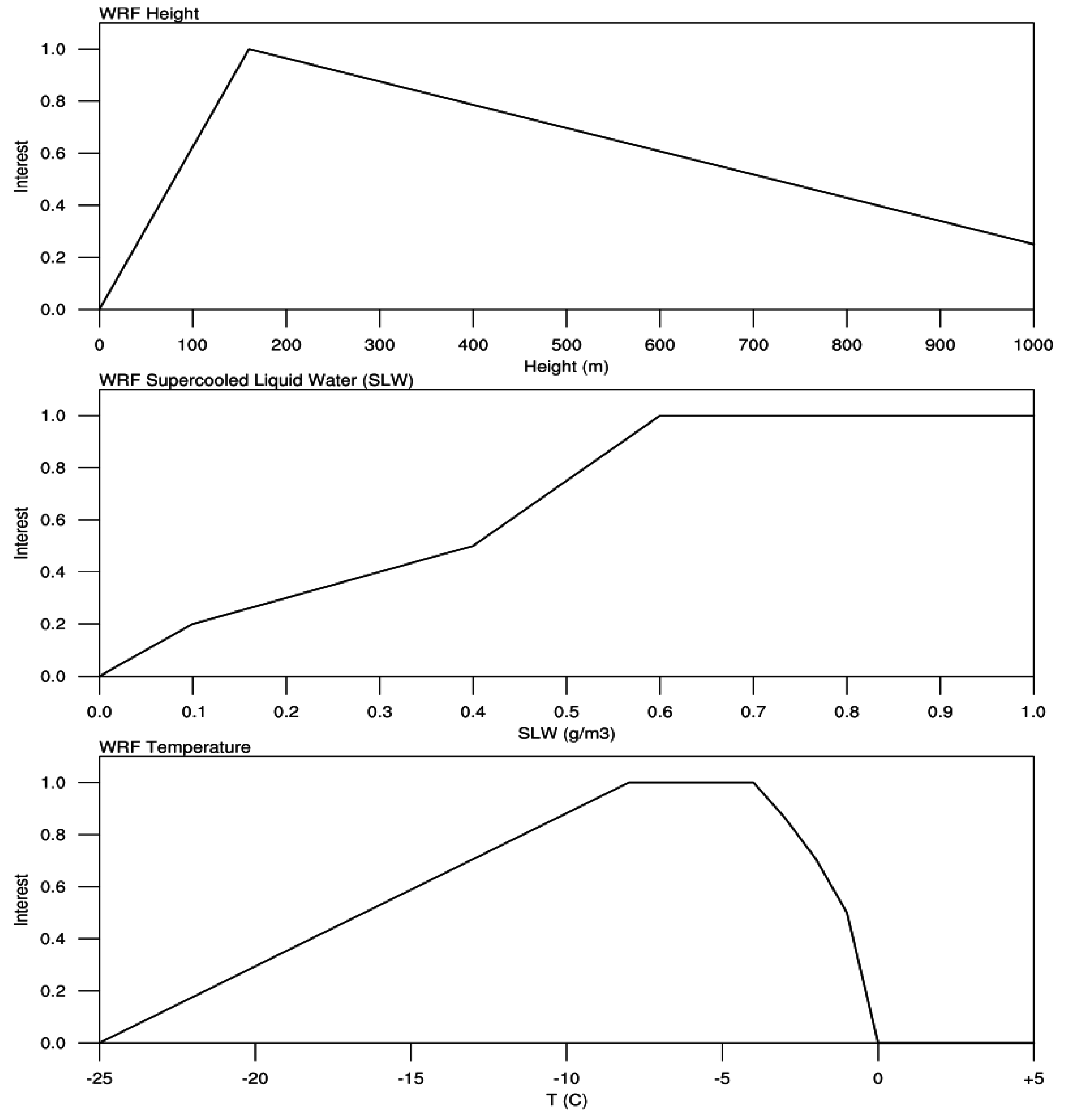
Figure 10 shows the relationship between three WRF output variables (height, temperature, and supercooled liquid cloud droplets and rain drops) used to compute the icing potential and the likelihood of icing for each one. The icing potential is computed at each height below a user-configured ceiling, above which icing conditions are not considered to have an effect at the hub-height. Icing potential is maximized when each of the three WRF output variables fall within their optimal range. As any of the three WRF output variables deviate from their optimal range, the icing potential decreases appropriately based on the slope of the curve for that variable. For DICast, values of CPOI above 0.4 will maximize the icing potential forecast. Both the WRF and DICast curves are configurable and customizable in order to cater to specific changes in input datasets and/or operator needs.
6.3. Wind and Temperature Forecasts
Maximum and minimum temperature forecasts are also provided by the ExWx. These forecasts again leverage both DICast and the WRF RTFDDA model output. Unlike for icing, both DICast and the WRF RTFDDA produce temperature forecasts natively at each grid box in the WRF and at each DICast site. This makes the combination of DICast and WRF temperature forecasts simpler than the icing forecasts. The other difference is that there is no derived variable provided to the operator; the temperature forecast is simply provided verbatim, and decisions about impacts are made at the display level. The same is true for high wind speed forecasts, which could be enhanced by adding a wind gust forecast.
6.4. Turbine Forecasts
To collect and present the data from the icing and temperature forecasts, a configurable system was developed to produce a value of the icing potential and temperatures (both maximum and minimum) at each individual wind turbine. The region of influence for both DICast forecast sites and WRF RTFDDA model grid boxes is configurable. Thus, if the underlying NWP model grid within the operating region changes the horizontal grid spacing or the number of DICast sites in an operating region increases or decreases, the user can adjust the size of these regions that influence an individual turbine accordingly.
Once the population of influencing points has been identified, the icing potential and temperature forecasts are combined to produce a single value for each wind turbine in the operating region. For icing potential forecasts, a percentile threshold is applied to all WRF RTFDDA model points and DICast points. The maximum forecast from either the DICast or the WRF is then chosen as the final icing potential forecast for that turbine, unless only a single input is available; in which case, the icing potential forecast for that turbine will simply be the icing potential forecast from whichever dataset is available. The percentile used to threshold the influencing data is also configurable. This allows for a dynamic system which enables wind farm operators to tailor the guidance to their preferences and experiences. For temperature forecasts, the average temperature of all DICast points in the immediate region and for WRF RTFDDA model points are computed separately. If both forecasts are available, then the final temperature forecast is the average of those two values; otherwise it is set to either the DICast or WRF forecast only, whichever is available. Additional processing can combine turbine output at the farm, node, or region level.
6.5. Case Study
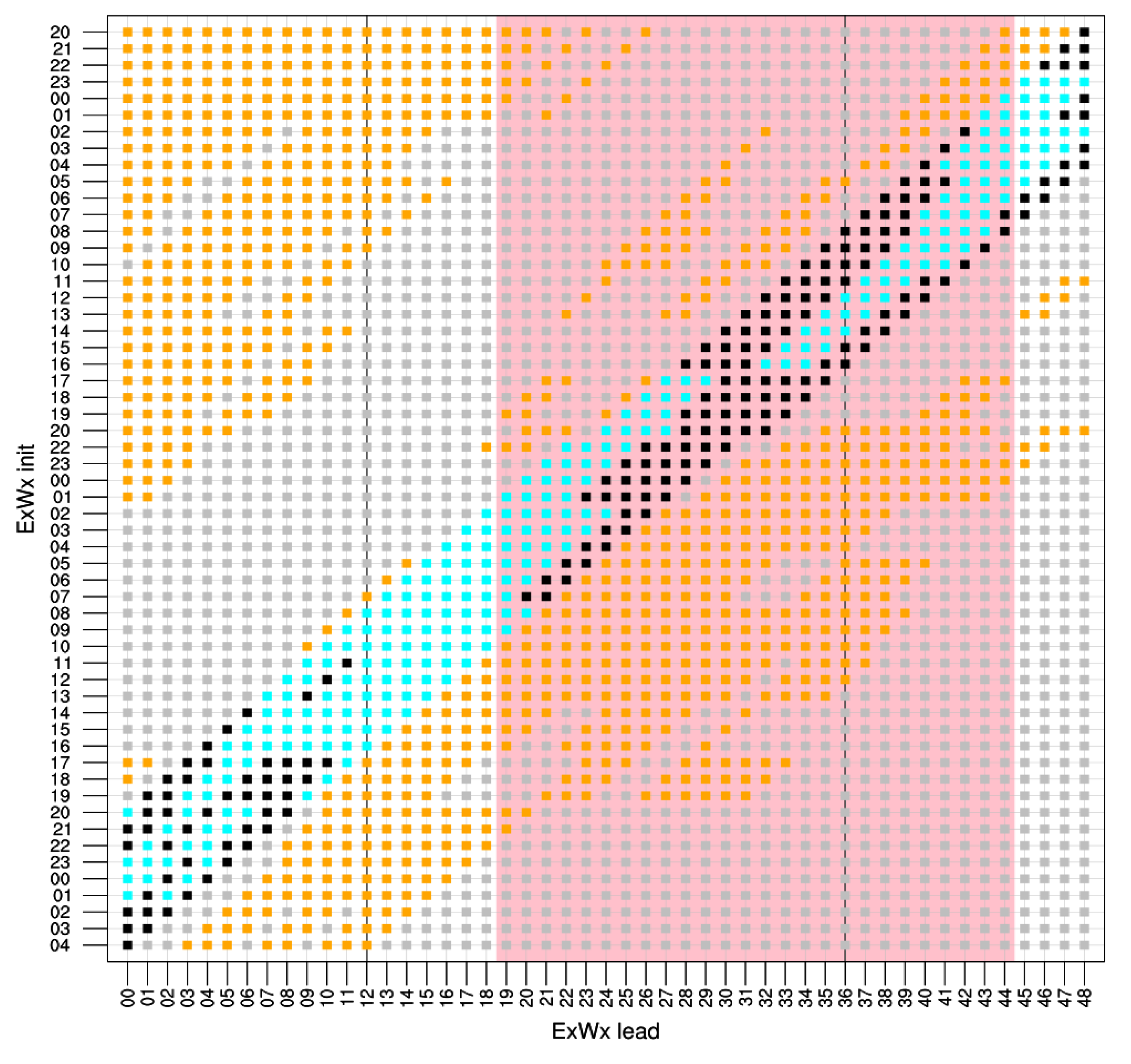
Since the extreme weather system runs hourly, it generates a new 0 to 72-h prediction every hour. ExWx performs optimally between hours 0 and 48, when both the DICast forecast system and WRF model output are available. As a case study, we analyze an icing event that occurred on 26 December 2014 at a wind farm located in Minnesota. The model output shown for this case combined forecasts at each of the turbines in the farm. Based on wind power and forecast outputs for the farm, the event window was chosen to be nine hours, centered on 0000 UTC on 26 December. Selecting a threshold of 0.5 for the icing potential highlights the capability of the system to predict the icing conditions at the wind farm up to 48 h prior to the event (
Figure 11).
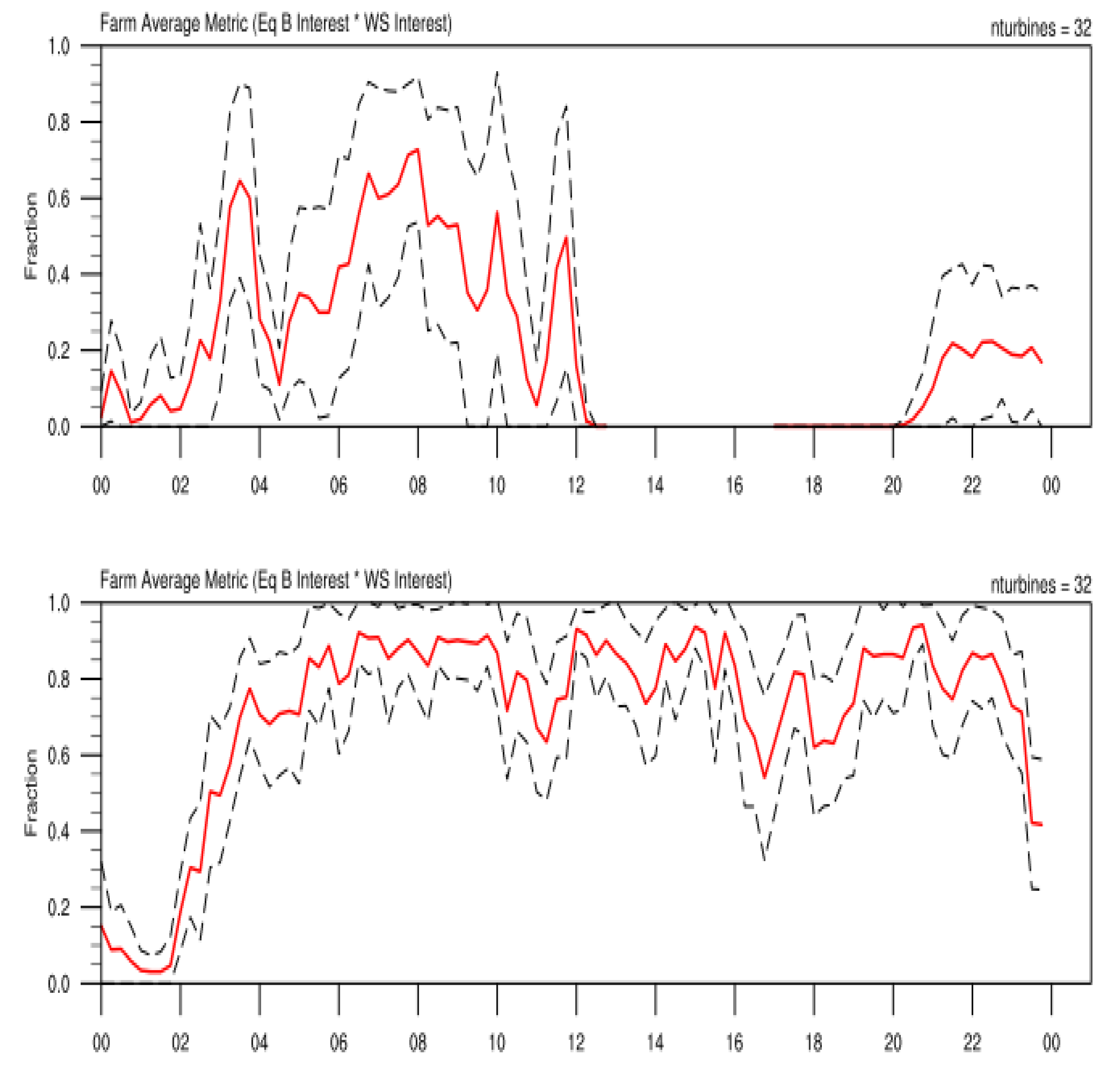
With limited truth data, robust statistical verification of the icing potential forecasts from the extreme weather system was challenging. Much of the initial configuration was based on nontraditional data sources, such as operator’s logs. In order to infer icing conditions, a metric was developed to identify them based on the wind turbine power output. This metric is simply a wind speed weighted ratio of the observed power to the expected power based on the turbine manufacturer’s power curve. This methodology must be used in conjunction with other data, such as icing sensors and/or operator-provided confirmation of icing conditions, in order to exclude those time periods when curtailment of the wind turbines may have occurred. Several possible icing periods are shown in
Figure 12. For the two days in this particular event, there appear to have been three distinct periods of possible icing conditions (
Figure 11). The ExWx forecasts of icing potential > 0.5 (
Figure 11) are roughly coincident with the decreased power production shown in
Figure 12. Additional information obtained from the operator confirmed that icing occurred during these time periods.
To provide the best configuration, a thorough database of known icing events provided via operator information and/or an icing sensor located at a wind farm is preferred. However, initial examination of several known icing cases shows promising performances of the system at alerting an operator of potential icing conditions with one to two days of lead time.
7. Conclusions
A comprehensive wind power forecasting system developed in collaboration with Xcel Energy integrates forecasting at a range of time scales utilizing an observation-based expert system and the radar assimilation model, VDRAS, for short-term forecasting and global model output with limited area high-resolution WRF RTFDDA modeling with several artificial intelligence approaches. The statistical, machine-learning system, DICast®, has been enhanced, as have the power conversion algorithms, through use of a regression tree algorithm and by deploying a quantile data quality control scheme. Finally, an AI analog ensemble approach provides both probabilistic information and improves upon the deterministic forecast. Additional modules provide estimates of extreme events, including icing, high winds, and extreme temperatures.
Xcel Energy is employing wind power forecasting for economic reasons, as it allows them to effectively integrate wind power into their operations. Since forecast errors are real costs in the energy market, more accurate forecasts can save utilities and their ratepayers substantial amounts of money. Xcel Energy estimates a savings of over
$60M in the past six years due to lowered day-ahead forecast errors. They depend on accurate forecasts more as their wind power capacity increases in order to integrate the variable wind resources into the grid more efficiently, economically, and reliably. Thus, highly accurate wind power forecasts enable renewable energy to effectively increase its fraction in the energy portfolio. These technologies have been reported at workshops and conferences [
27], where they generate interest and are picked up by commercial forecast providers.
Author Contributions
Conceptualization, B.K. and S.E.H.; methodology, D.A., G.W., L.D.M., Y.L., S.L., and M.P.; software, P.P.; validation, T.J.; formal analysis, D.A., S.A., W.C., and S.L.; investigation, S.A. and G.W.; resources, S.E.H. and G.W.; data curation, G.W., S.L., and P.P.; writing—original draft preparation, B.K. and S.E.H.; writing—review and editing, B.K. and S.E.H.; visualization, B.K., D.A., S.A., G.W., L.D.M., S.L., and W.C.; supervision, S.E.H.; project administration, S.E.H.; and funding acquisition, S.E.H. All authors have read and agreed to the published version of the manuscript.
Funding
This research was funded by Xcel Energy.
Acknowledgments
The authors gratefully acknowledge the contributions of the rest of the project team and of the Xcel Energy oversight team.
Conflicts of Interest
The authors declare no conflicts of interest.
References
- Mahoney, W.P.; Parks, K.; Wiener, G.; Liu, Y.; Myers, W.L.; Sun, J.; Monache, L.D.; Hopson, T.; Johnson, D.; Haupt, S.E. A Wind Power Forecasting System to Optimize Grid Integration. IEEE Trans. Sustain. Energy 2012, 3, 670–682. [Google Scholar] [CrossRef]
- Haupt, S.E.; Mahoney, W.P.; Parks, K. Wind Power Forecasting; Springer Science and Business Media LLC: New York, NY, USA, 2014; pp. 295–318. [Google Scholar]
- Haupt, S.E.; Mahoney, W.P.; Parks, K. Wind Power Forecasting. Weather Matters Energy 2014, 295–318. [Google Scholar]
- Giebel, G.; Kariniotakis, G. Best Practice in Short-term Forecasting—A Users Guide. In Proceedings of the European Wind Energy Conference and Exhibition, Milan, Italy, 7–10 May 2007. [Google Scholar]
- Monteiro, C.; Bessa, R.; Miranda, V.; Botterud, A.; Wang, J.; Conzelmann, G.; Porto, I. Wind power forecasting: State-of-the-art 2009. In Proceedings of the Argonne National Laboratory, Argonne, IL, USA, 20 November 2009. [Google Scholar]
- Ahlstrom Jone, L.; Zavadil, R.; Grant, W. The future of wind forecasting and utility operations. IEEE Power Energy Mag. 2005, 3, 57–64. [Google Scholar] [CrossRef]
- Wilczak, J.; Finley, C.; Freedman, J.; Cline, J.; Bianco, L.; Olson, J.; Djalalova, I.; Sheridan, L.; Ahlstrom, M.; Manobianco, J.; et al. The Wind Forecast Improvement Project (WFIP): A Public-Private Partnership Addressing Wind Energy Forecast Needs. Bull. Am. Meteorol. Soc. 2015, 96, 1699–1718. [Google Scholar] [CrossRef]
- Gneiting, T.; Larson, K.; Westrick, K.; Genton, M.G.; Aldrich, E. Calibrated Probabilistic Forecasting at the Stateline Wind Energy Center. J. Am. Stat. Assoc. 2006, 101, 968–979. [Google Scholar] [CrossRef]
- Ding, Y. Data Science for Wind Energy, 1st ed.; CRC: Boca Raton, FL, USA, 2019; p. 424. [Google Scholar]
- Skamarock, W.C.; Klemp, J.B.; Dudhia, J.; Gill, D.O.; Barker, D.M.; Duda, M.G.; Huang, X.-Y.; Wang, W.; Powers, J.G. A Description of the Advanced Research WRF Version 3; NCAR Tech Note NCAR/TN 475 STR; National Center for Atmospheric Research: Boulder, CO, USA, 2008; p. 125. [Google Scholar]
- Benjamin, S.G.; Weygandt, S.S.; Brown, J.M.; Hu, M.; Alexander, C.; Smirnova, T.G.; Olson, J.B.; James, E.; Dowell, D.C.; Grell, G.A.; et al. A North American Hourly Assimilation and Model Forecast Cycle: The Rapid Refresh. Mon. Weather. Rev. 2016, 144, 1669–1694. [Google Scholar] [CrossRef]
- Liu, Y.; Warner, T.; Swerdlin, S.; Betancourt, T.; Knievel, J.; Mahoney, B.; Pace, J.; Rostkier-Edelstein, D.; Jacobs, N.A.; Childs, P.; et al. NCAR ensemble RTFDDA: Real-time operational forecasting applications and new data assimilation developments. In Proceedings of the 24th Conference on Weather Analysis and Forecasting and the 20th Conference on Numerical Weather Prediction, Seattle, WA, USA, 11–15 January 2011. [Google Scholar]
- Antoniou, I.; Pedersen, T.F. Nacelle Anemometry on a 1 MW Wind Turbine: Comparing the Power Performance Results by Use of the Nacelle or Mast Anemometer; Risø Report Risø-R-941(EN); Forskningscenter Risø: Roskilde, Denmark, 1997; p. 34. [Google Scholar]
- Smith, B.; Link, H.; Randall, G.; McCoy, T. Applicability of Nacelle Anemometer Measurements for Use in Turbine Power Performance Tests; National Renewable Energy Laboratory preprint NREL/CP-500-32494; National Renewable Energy Laboratory: Golden, CO, USA, 2002. [Google Scholar]
- Cheng, W.Y.; Liu, Y.; Bourgeois, A.J.; Wu, Y.; Haupt, S.E. Short-term wind forecast of a data assimilation/weather forecasting system with wind turbine anemometer measurement assimilation. Renew. Energy 2017, 107, 340–351. [Google Scholar] [CrossRef]
- Myers, W.; Wiener, G.; Linden, S.; Haupt, S.E. A consensus forecasting approach for improved turbine hub height wind speed predictions. In Proceedings of the WindPower 2011, Anaheim, CA, USA, 24 May 2011. [Google Scholar]
- Gneiting, T.; Katzfuss, M. Probabilistic Forecasting. Annu. Rev. Stat. Its Appl. 2014, 1, 125–151. [Google Scholar] [CrossRef]
- Monache, L.D.; Eckel, F.A.; Rife, D.L.; Nagarajan, B.; Searight, K. Probabilistic Weather Prediction with an Analog Ensemble. Mon. Weather Rev. 2013, 141, 3498–3516. [Google Scholar] [CrossRef]
- Alessandrini, S.; Monache, L.D.; Sperati, S.; Nissen, J. A novel application of an analog ensemble for short-term wind power forecasting. Renew. Energy 2015, 76, 768–781. [Google Scholar] [CrossRef]
- Ezzat, A.A.; Jun, M.; Ding, Y. Spatio-temporal short-term wind forecast: A calibrated regime-switching method. Ann. Appl. Stat. 2019, 13, 1484–1510. [Google Scholar] [CrossRef]
- Junk, C.; Delle Monache, L.; Alessandrini, S.; Cervone, G.; von Bremen, L. Predictor-weighting strategies for probabilistic wind power forecasting with an analog ensemble. Meteorol. Z. 2015, 24, 361–379. [Google Scholar] [CrossRef]
- Sun, J.; Crook, N.A. Dynamical and Microphysical Retrieval from Doppler Radar Observations Using a Cloud Model and Its Adjoint. Part I: Model Development and Simulated Data Experiments. J. Atmos. Sci. 1997, 54, 1642–1661. [Google Scholar] [CrossRef]
- Sun, J.; Chen, M.; Wang, Y. A Frequent-Updating Analysis System Based on Radar, Surface, and Mesoscale Model Data for the Beijing 2008 Forecast Demonstration Project. Weather. Forecast. 2010, 25, 1715–1735. [Google Scholar] [CrossRef]
- Bernstein, B.C.; McDonough, F.; Politovich, M.K.; Brown, B.G.; Ratvasky, T.P.; Miller, D.R.; Wolff, C.A.; Cunning, G. Current Icing Potential: Algorithm Description and Comparison with Aircraft Observations. J. Appl. Meteorol. 2005, 44, 969–986. [Google Scholar] [CrossRef]
- McDonough, F.; Bernstein, B.C.; Politovich, M.K.; Wolff, C.A. The forecast icing potential (FIP) algorithm, Preprints. In Proceedings of the 20th International Conference on Interactive Information and Processing Systems (IIPS) for Meteorology, Oceanography, and Hydrology, Seattle, WA, USA, 14 January 2004. [Google Scholar]
- Thompson, G.; Field, P.; Rasmussen, R.M.; Hall, W.D. Explicit Forecasts of Winter Precipitation Using an Improved Bulk Microphysics Scheme. Part II: Implementation of a New Snow Parameterization. Mon. Weather. Rev. 2008, 136, 5095–5115. [Google Scholar] [CrossRef]
- Kosovic, B.; Haupt, S.E.; Wiener, G.; Delle Monache, L.; Liu, Y.; Linden, S.; Politovich, M.; Sun, J. Scientific Advances in Wind Power Forecasting. In Proceedings of the American Wind Energy Association, Orlando, FL, USA, 21 May 2015. [Google Scholar]
Figure 1.
Flowchart of the National Center for Atmospheric Research’s (NCAR’s) Xcel Energy power prediction system. NCEP: U.S. National Centers for Environmental Prediction, NAM: North American model, GFS: global forecasting system, RUC: Rapid Update Cycle, GEM Global Environmental Multiscale model, WRF RTFDDA: Weather Research and Forecasting-based real-time four-dimensional data assimilation, and VDRAS: variational doppler radar analysis system.
Figure 2.
Comparison of hourly data assimilation and forecasting cycles without (left panel) and with (right panel) assimilation of wind turbine hub-height wind speed observations for a large wind farm in Northern Colorado. The black lines show the mean wind. Different color lines represent forecasts from different cycles with the first (last) two digits in the legend denoting the day of the month (hour in UTC). Conventional obs DA: conventional observation data assimilation and farm ws DA: farm wind speed data assimilation.
Figure 3.
Comparison of the performance of RTFDDA with baseline numerical weather prediction (NWP) models. MAE: mean absolute error.
Figure 3.
Comparison of the performance of RTFDDA with baseline numerical weather prediction (NWP) models. MAE: mean absolute error.
Figure 4.
Power curve for a wind farm indicating percentile curves.
Figure 4.
Power curve for a wind farm indicating percentile curves.
Figure 5.
Example of an analog ensemble forecast probability density function (PDF) over one station of the dataset. The blue shadings correspond to the 25–75 (darker) and 5–95 (lighter) quantiles. The black and yellow dashed lines represent the wind speed observations and AnEn ensemble mean, respectively. The red line is the DICast wind speed forecast. AnEn: analog ensemble.
Figure 6.
Root mean square error (RMSE) as a function of forecast lead time for DICast (red) and AnEn means (black) computed over all stations. Bootstrap 5%–95% confidence intervals are plotted for AnEn only. RMSE values listed are computed by including all lead times.
Figure 6.
Root mean square error (RMSE) as a function of forecast lead time for DICast (red) and AnEn means (black) computed over all stations. Bootstrap 5%–95% confidence intervals are plotted for AnEn only. RMSE values listed are computed by including all lead times.
Figure 7.
Brier skill score (BSS) of the analog ensemble (AnEn) with DICast as a reference, as a function of forecast lead time, computed over all the stations. The BSS 5%–95% bootstrap confidence intervals are also shown. The event considered is wind speed greater than 10 ms−1.
Figure 7.
Brier skill score (BSS) of the analog ensemble (AnEn) with DICast as a reference, as a function of forecast lead time, computed over all the stations. The BSS 5%–95% bootstrap confidence intervals are also shown. The event considered is wind speed greater than 10 ms−1.
Figure 8.
Schematic of the observations-based expert system for short-term forecasting. Available wind speed observations at 10 m in concentric circles around a wind farm are used to calculate the wind ramp metric, which is then used to compute changes in power production.
Figure 8.
Schematic of the observations-based expert system for short-term forecasting. Available wind speed observations at 10 m in concentric circles around a wind farm are used to calculate the wind ramp metric, which is then used to compute changes in power production.
Figure 9.
Summary schematic visualizing the various input datasets to the extreme weather system (ExWx). For DICast, C1-C4 indicate various configurations of the DICast forecast that are dependent on the input model data available at that lead time.
Figure 9.
Summary schematic visualizing the various input datasets to the extreme weather system (ExWx). For DICast, C1-C4 indicate various configurations of the DICast forecast that are dependent on the input model data available at that lead time.
Figure 10.
Curves representing the interest in icing conditions (0–1) for three variables from the WRF RTFDDA model data. Top panel is height of the model level, middle panel represents supercooled liquid water, (i.e., liquid rain or cloud drops below freezing), and the bottom panel shows temperature. The intersection of the three curves where they return a value of 1 will maximize the icing potential from the WRF RTFDDA model data. SLW: supercooled liquid water.
Figure 11.
Forecasts of icing potential, combined from all turbines on a single farm, from 57 consecutive runs of the extreme weather system (y-axis). The first run shown is the 2000 UTC forecast from the extreme weather system on 24 December, 2014. Black shading indicates valid times within the event window (2000 UTC on 25 December–0400 UTC on 26 December) with an icing potential forecast of < 0.5, light blue shading indicates an icing potential forecast of > 0.5 within the event window, orange shading indicates an icing potential forecast of > 0.5 outside the event window, and gray shading indicates an icing potential forecast of < 0.5 outside the event window. Vertical lines indicate the division between C1, C2, and C3 DICast forecast system data (see
Figure 9).
Figure 12.
Wind speed weighted metric to identify periods when power production was less than expected and wind speeds were high enough to have confidence in the manufacturer’s power curve (i.e., not in the lower tail of the curve). The red line shows the farm average, while the black dashed lines show +/- the standard deviation for the farm. Top panel is for 25 December 2014, and bottom panel is for 26 December 2014. Higher values indicate a higher likelihood of icing (or curtailment).
© 2020 by the authors. Licensee MDPI, Basel, Switzerland. This article is an open access article distributed under the terms and conditions of the Creative Commons Attribution (CC BY) license (http://creativecommons.org/licenses/by/4.0/).

 ,
, 


