Validation of Novel PLL-driven PI Control Schemes on Supporting VSIs in Weak AC-Connections

Abstract

The integration of distributed energy resources (DERs) in modern power systems has substantially changed the local control capabilities of the grid since the majority of DERs are connected through a controlled dc/ac inverter interface. Such long-distance located DER installations, usually represented by current regulated dc sources, can inject large amounts of power into the main ac grid at points where the strength of the ac connection is low. The efficient and stable performance of such a power scheme is related to the capability of the control applied to retain the power extraction close to the maximum and simultaneously to regulate the dc-side voltage as well as the ac-side voltage magnitude at the weak ac connection point. This is implemented by designing the controllers of the voltage source inverters (VSIs) in a manner that reliably satisfies the above tasks. To this end, decentralized cascaded control schemes, driven by novel, locally implemented phase locked loops (PLLs), suitable to work in weak ac connections, are proposed for the VSI performance regulation by using new fast inner-loop proportional-integral (PI) current controllers. A decisive innovation is proposed by inserting an extra damping term in the inner-loop controllers to guarantee stability and convergence to the desired equilibrium. This is analytically proven by a rigorous analysis based on the entire nonlinear system model, where advanced Lyapunov-based methods are deployed in detail. As a good transient response of the VSI interface is indeed critical for the energy and grid system management, the conducted simulation and experimental results confirm that the proposed scheme efficiently supports the ac- and dc-side voltages of the VSI under different varying conditions in the power production or any voltage changes of the main grid.

1. Introduction

Over the last hundred years, the increase of energy production has substantially improved human life while simultaneously has had a highly negative impact on the global environmental conditions. Due to these reasons, nowadays, different actions, such as the 2030 Framework for Climate and Energy [1] and the 2030 Agenda for Sustainable Development [2], have set clear goals of achieving sustainable management of the natural resources and taking urgent action on climate change, so that the needs of the present and future generations can be supported. In this frame, the conventional centralized electric power system is gradually changing due to the increasing penetration of renewable energy sources (RES) and other distributed energy resources (DERs). The scheme of distributed generation (DG), involving large DER installations such as wind farms or photovoltaic stations, has already been implemented within the power grid, serving a considerable percentage of the total power demands. As DG deployment is, in most cases, realized by connecting DER units to the main grid through power converter interfaces [3], this enables local, decentralized controls to be applied [4,5] which are used to match the system operational requirements and simultaneously to regulate the injecting power to the grid as well.

In this scheme, voltage source inverters (VSIs) are used as standard controlled interfaces [6]. Hence, the key role of VSIs is evident and their contribution to the overall system performance and stability becomes crucial. In turn, a critical aspect of efficient and stable operation of a grid-tied VSI is based on whether it is ultimately connected to a strong and stiff ac-power grid or to a weak one [7]. In fact, the latter is often the case since DER installations are usually geographically dispersed in a wide area, far from the main grid electricity production.

As it is well known, grid strength generally describes how rigid a grid reaction is to small perturbations or disturbances and depends heavily on its impedance and rotating inertia. The stiffness of a grid is numerically expressed by the short circuit ratio (SCR) [6], referred to a certain point of common coupling (PCC). This particular index is defined as the ratio of the short-circuit capacity at a given grid point to the rated power of the interconnected power converter. Typical values of SCR indicating weak grid interfaces are less than 3 ($\mathrm{S}\mathrm{C}\mathrm{R} \le 3$), and as SCR approaches to unity, the grid is characterized as very weak and that is in fact the worst case scenario for the system performance [8,9].

A fairly common example of low valued-SCR can be caused by a connection to a high-impedance grid through long cables. In such cases, the VSI terminal voltage is susceptible to disturbances from both the VSI itself and the grid, while the control loops implemented on the power electronic interface affect the output voltage dynamics and vice versa. Moreover, weak ac-grid connections introduce further limitations to the maximum amount of available power that can be injected to the grid, whereas the equivalent grid impedance is often time-varying as a result of faults or load power variations [10]. Nevertheless, as common as these cases may be, they certainly present concurrent engineering challenges and still have open problems to be studied. In particular, when DERs are connected to weak ac-grids, a cumbersome analysis is usually needed which includes dynamic analysis, control design and stability verification [11,12].

In Reference [13], it is studied the impact of phase-locked loop (PLL) on impedance modeling and resonance in a doubly fed induction generator RES with a parallel compensated weak grid. In Reference [14], a thorough analysis of the effect mechanism of frequency variation on the weak grid-connected VSI system stability in a dc voltage control timescale is presented. In Reference [15], the stability of multiple DERs that are connected in parallel to a weak ac grid is analyzed. In all the aforementioned works, the small-signal model of the system is used which however is unable to guarantee stability under large disturbances. Another very interesting technique that allows the design of robust controllers for systems vulnerable to disturbances, such as weak ac grids, is the nonlinear H-infinity control method. However, this theory suffers from the lack of a systematic method of solving the resulting inequalities that arise in the case of complex nonlinear systems [16]. To overcome this obstacle, usually a small-signal model is used [17] or some kind of heuristic algorithms [18]. Certainly, in these cases, the control design once again is not based on the accurate nonlinear model and stable operation can be guaranteed only for predetermined operating points.

To confront some fundamental problems of the aforementioned ones, in this paper, the nonlinear dynamic behavior of a fully controlled VSI system is studied and reviewed under the case of feeding power from a remotely allocated DER to a weak ac grid. Keeping in mind the difficulties introduced, the main objective is to design novel control schemes to effectively regulate both the ac- and dc-side voltage of the VSI interface and to ensure stable and seamless power transfer to the grid. These particular tasks are accomplished by implementing a cascaded type of control scheme, where inner-loop current regulators are driven by outer-loop ac- and dc-voltage controllers. It must be noted that significant innovations are considered in the whole design: Firstly, the proposed inner-loop control laws are simplified without needing the commonly involved decoupling terms as introduced in conventional designs [19,20]. Hence, their structure is of a pure proportional-integral (PI) type and they provide the power converter duty-ratio inputs in a direct way, avoiding a division by the dc voltage state variable as encountered in common control design practices, whereas extra damping terms are additionally implemented in the integrator loops contributing to system stability without affecting the accuracy of the regulation. Secondly, the PLL drive circuit is suitably modified in order to provide a response independent of the different ac-side voltage variations. This is a crucial design modification, since it makes it possible to effectively connect VSIs in weak ac-grid points. To that end, the ac voltage reference magnitude of the outer-loop controller is used in the PLL instead of the original ac voltage magnitude, while the latter is used only for the angle assignment. It is, therefore, evident that the cascaded controllers’ smooth and stable response is essential to the PLL operation. As a result, the fast dynamics of the inner-loop controllers have to be incorporated into the whole system analysis, since the validation of stability is a fundamental preliminary for the efficient performance of the whole system operation. Indeed, this analysis proves the system overall stability and guarantees that all its states converge to the desired equilibrium.

The remainder of the paper is organized as follows. In Section 2, the whole system structure is given, and the targets and the methodologies are presented. In Section 3, we start with the system modeling and we continue with the controller and system analysis. Stability is also analyzed with the current-loop controllers incorporated in the original dynamic model to formulate the closed-loop version of the system. In Section 4, the verification of the desired performance of the VSI is conducted and the simulation and the detailed experimental results are discussed. In Section 5, future work directions are given, while in Section 6, some conclusions are drawn.

2. System Structure, Targets and Methodologies

In this section, first, the complete system structure is presented in the form of interconnected circuit subsystems i.e., the feeding DER, the controlled VSI interface and the ac-grid configuration. Additionally, the main targets considered in the scope of the present study are determined, whereas the methods employed in order to achieve these crucial goals are also described in the last subsection.

2.1. System Structure

Figure 1 depicts the system under consideration, where a DER is connected to the grid via a VSI interface. Central role in this kind of configurations plays the power converter interface, which is represented by a standard three-phase VSI comprising six IGBT elements. The three-phase dc/ac VSIs are the widest used power electronic devices in industrial applications and renewable energy systems. They are effectively used as prime controlled input interfaces with aim to regulate the dc-side voltage as well as the ac-side voltage magnitude at the ac connection point in cases of weak ac grid connections.

On the dc-side, a DER is connected providing power to the grid through the VSI. It is noted that DERs can effectively represent large wind or photovoltaic stations or any other strongly output current-regulated power source. Therefore, in our case, the DER is modeled abstractly as a controlled current source, with variable magnitude due to its intermittent nature, as considered in dc grids [21].

On the ac-side, the VSI can either be connected to a strong ac grid or to weak one. An ac-grid featuring infinite inertia and robust capabilities of withstanding significant perturbations (sudden power or voltage changes) is characterized as a strong one. On the contrary, weak ac grids display reduced capabilities on resisting and overcoming voltage disturbances. Generally, an ac system, at a particular node, can be considered weak either due to its low inertia or to its high impedance [7]. In our case, the VSI is supplying power to the PCC on the bus where the capacitor bank $C_B$ is connected via an R-L filter. The PCC itself is connected to the actual main ac grid through a long line. This leads to an increased grid impedance (weak ac connection) which may exhibit low damping characteristics during voltage fluctuations and frequency oscillations.

The crucial role in maintaining VSI synchronism is implemented by the PLL action, which provides the voltage angle at the PCC bus. This standard technique for strong ac grid connections, is used to transform the three-phase ac voltage and current quantities into d-q synchronously rotating dc components. A main innovation introduced in this paper is related with the PLL implementation, by making this suitable also for weak ac connections, as explained in the following section.

The whole system structure is completed by the modified PI inner-loop controllers which are driven by the PLL mechanism and are commanded by suitable outer-loop voltage regulators. The controllers’ tasks are explained in the following subsection, whereas the innovations introduced to increase their capability on maintaining stability are discussed in Section 3.

2.2. Main Objectives and Tasks

The main target of this paper is to examine the dynamic behavior of a VSI system that is used to connect a remotely located DER to the main ac grid. Due to the connection through long cables usually employed in these cases, a weak connection point is typically considered. Contrary to the case of a strong ac-grid connection, in a weak ac-grid connection, the ac voltage at the inverter output is not constant anymore. Therefore, another important objective is to design a control scheme for VSIs that can support the ac-side voltage by maintaining it at a desired constant value regardless of the DER current injected to the grid. However, as the VSI control has to be implemented locally, this is not an easy task, since the reference ac-voltage is now far from the PCC at the infinite bus on the opposite end of a long-distance line. It is well-known that a reliable local feedback scheme for the VSI is well-defined only in the case of a strong ac grid connection, hence a final target is to implement a suitable PLL synchronization mechanism that can reliably support the local feedback scheme for the weak ac connection case. Nevertheless, it is evident that the whole system has to be examined for its stability, since in the case of weak ac grid connections, the controller performance has a decisive action. Our main objective is to design applicable and easily implemented drive schemes, with a trade-off being adopted between stable performance and simple controller structures.

2.3. Methods

In our analysis, the accurate nonlinear model of the examined system is derived through the application of suitable modeling methods based on the synchronously rotating d-q frame representation and the mean-value modeling technique for the VSI [22]. Additionally, for the control design, the cascaded mode control method is adopted [23] that can lead to parameter-free and robust controllers. To validate the stable behavior of the system, instead of applying standard small-signal-based techniques, Lyapunov-based methods are utilized that take into consideration all the nonlinearities. It is noticed that the Lyapunov-based methods are carefully applied in order to maintain simple and friendly to industrial engineers control schemes with a clear cost on the analysis effort. This provides the opportunity of designing a closed-loop system which is independent from the operating point, simultaneously avoiding inaccurate solutions. Finally, a combination of simulation and experimental methods are employed in order to evaluate both the transient and steady-state performance of the system under the action of the implemented control scheme.

3. Model Description, System Analysis and Experimental Setup

The whole modeling is developed on the synchronously rotating d-q reference frame [6], where the three-phase ac-variables conveniently become dc-quantities in steady-state, whereas the featured nonlinear VSI model is derived through the adoption of the well-known mean value method [22].

3.1. VSI-Based Modeling and Control of DERs Connected to the Grid

The dynamic model of the subsystem including the VSI interface is expressed in the synchronously rotating d-q reference frame, [24,25], as:

$$L_f{\dot{I}}_d=-R_f{I}_d+{\omega }_{PLL}{L}_f{I}_q+m_d{V}_{dc}-V_{db}$$

(1)

$$L_f{\dot{I}}_q=-{\omega }_{PLL}{L}_f{I}_d-R_f{I}_q+m_q{V}_{dc}-V_{qb}$$

(2)

$$\frac{2}{3}{C}_{dc}{\dot{V}}_{dc}=-\left(m_d{I}_d+m_q{I}_q\right)-\frac{V_{dc}}{R_{dc}}+\frac{2}{3}{I}_{dc}$$

(3)

where $I_d$ and $I_q$ are the d and q-axis components of the VSI output currents $I_a$,$I_b$,$I_c$, along with $V_{dB}$ and $V_{qB}$, which are the corresponding components of the ac voltages at the PCC. The dc-voltage at the dc-side capacitor $C_{dc}$ is denoted by $V_{dc}$, with its parallel parasitic resistance denoted by $R_{dc}$, while $I_{dc}$ represents the dc-current source. The d- and q-axis components of the switching duty-ratios of the IGBT switching elements are expressed as $m_d(=V_d/V_{dc})$ and $m_q(=V_q/V_{dc})$ respectively, representing the controlled inputs of the VSI, in the d-q reference frame (where $V_d$ and $V_q$ stand for the d- and q-axis components of the inverter ac-side voltages $V_a$, $V_b$, $V_c$). The filter resistance and inductance are denoted by $R_f$ and $L_f$ respectively, where ${\omega }_{PLL}$ is the angular frequency provided by a suitable PLL circuit.

Following the d-q reference frame representation, the actual active and reactive power injected by the VSI are then given by:

$$P_{PCC}=\frac{3}{2}\left(V_{dB}{I}_d+V_{qB}{I}_q\right)$$

(4)

$$Q_{PCC}=\frac{3}{2}\left(V_{qB}{I}_d-V_{dB}{I}_q\right)$$

(5)

3.2. Weak AC-Grid Interface

As the ac-system impedance increases, the voltage magnitude at the connecting PCC in general will become more sensitive to power variations of the connected generation source. Furthermore, the injected power to the grid is expected to be significantly decreased. In our case, the SCR index is defined as:

$$SCR=\frac{S_{ac}}{P_N}$$

(6)

where $S_{ac}$ is the short-circuit power capacity of the ac grid and $P_N$ is the nominal power offered by the VSI.

Keeping in mind that $S_{ac}$ represents the total magnitude of a three-phase short circuit to the ground at the PCC, its value can only be theoretically assumed. In fact, the grid has to be modeled as a Thevenin-equivalent voltage source in order to obtain the value of $S_{ac}$ as:

$$S_{ac}=\frac{V_B^2}{Z_{th}}$$

(7)

where $\left|V_B\right|$ is the voltage magnitude at the PCC and $Z_{th}$ is the Thevenin impedance, which in turn depends on the grid inductance $L_g$. Obviously, the inclusion of a long line between the PCC and the actual ac system further increases $L_g$, which has an apparent effect on decreasing the SCR value. In particular, Figure 1 depicts the connection of a DER through a VSI interface to a PCC which is connected to the grid via a long line with resistance $R_{Line}$ and inductance $L_{Line}$ in series.

Completing, therefore, the dynamic model in the d-q reference frame at the ac-side by taking into account the line configuration, we obtain:

$$C_B{\dot{V}}_{dB}=I_d-\frac{V_{dB}}{R_B}+{\omega }_{PLL}{C}_B{V}_{qB}-I_{dLine}$$

(8)

$$C_B{\dot{V}}_{qB}=I_q-\frac{V_{qB}}{R_B}-{\omega }_{PLL}{C}_B{V}_{dB}-I_{qLine}$$

(9)

$$L_{Line}{\dot{I}}_{dLine}=V_{dB}-R_{Line}{I}_{dLine}+{\omega }_{PLL}{L}_{Line}{I}_{qLine}-V_{dGrid}$$

(10)

$$L_{Line}{\dot{I}}_{qLine}=V_{qB}-R_{Line}{I}_{qLine}-{\omega }_{PLL}{L}_{Line}{I}_{dLine}-V_{qGrid}$$

(11)

where $I_{dLine}$ and $I_{qLine}$, and $V_{dGrid}$ and $V_{qGrid}$ represent the d- and q-axis components of the connecting line flowing currents and the infinite bus voltages respectively, while $R_B$ stands for a parallel resistive local load set at the PCC, and $C_B$ represents the capacitance at the same point, respectively.

It is worth noting that the system model given by Equations (1)–(3) and (8)–(11) represents a single DER connected at the PCC through a long line to a node with constant voltage. Nevertheless, it becomes apparent that the case of multiple DERs can be handled in a similar manner for each of them, if every DER is connected radially at the PCC and therefore the assumption of a single DER is adequate. Certainly, the case of more complex distribution networks with several DERs connected in arbitrary positions needs a more specific modeling, but in general, the PLL-driven scheme and the local controllers’ design can follow the same guidelines of analysis as that proposed in the next sections.

3.3. The Proposed Control and PLL Design

For the complete proposed design, the decentralized cascaded-mode control is adopted, which involves fast inner-loop current controllers, driven by slower outer-loop regulators. The proposed control scheme for the grid-tied inverter is included in Figure 1.

The aim of two proposed cascaded controllers applied on the d- and q-duty-ratio input respectively, is twofold:

1.  Firstly, to regulate the ac grid-side voltage magnitude at the desired level by introducing the following ac-voltage outer-loop PI regulator:

$$u_{ac}^{*}=k_{PV}(\frac{\left|V_B\right|}{V_B^{ref}}-1)+k_{IV}{\displaystyle {\int }_0^t(}\frac{\left|V_B\right|}{V_B^{ref}}-1)d\tau$$

(12)

with the magnitude of the ac-bus voltage calculated as $\left|V_B\right|=\sqrt{V_{dB}^2+V_{qB}^2}$.

To implement the cascaded-mode control structure, the following d-axis inner-loop current controller is proposed:

$$m_d=-k_{Pd}\left(I_d-I_d^{ref}\right)-k_{Id}{Z}_d$$

(13)

where the command input is taken as $I_d^{ref}=u_{ac}^{*}$ and it is determined by the output of the aforementioned outer-loop voltage controller, whereas $Z_d$ state is given by:

$${\dot{Z}}_d=I_d-I_d^{ref}-k_{If}{Z}_d$$

(14)

Obviously, Equation (14) represents the integrator term of the PI controller (Equation (13)), where now an additional damping term $k_{If}{Z}_d$ has been inserted. As shown in Section 3.5, the addition of the damping term is crucial to guarantee stable system performance. On the other hand, this modification does not affect the cascaded controller performance and it constitutes a very light change since it is implemented locally by feeding-back the inner-loop state $Z_d$. This is a significantly simpler solution compared to the standard decoupling methods [6], where the inserted feedback and feedforward terms are strongly dependent from the specific system structure, operating conditions and parameters.

All the d-q voltage and current components are provided by aligning the synchronously rotating d-q reference frame by a locally implemented PLL, as depicted in Figure 1. Normally, in a strong ac-bus, the PLL mechanism eliminates the frequency difference between the grid’s actual angular frequency ${\omega }_0$ and the angular frequency provided by the PLL circuit ${\omega }_{PLL}$, which is noted as:

$$\dot{\theta }={\omega }_{PLL}-{\omega }_0$$

(15)

and synchronizes its operation with the phase of the bus ac-voltages by zeroing-out one of the d- or q-axis voltage components (in our case the d-axis voltage component). Therefore, the dynamics of the system with the PLL control in state-space is given as in reference [26]:

$$\dot{\theta }=-k_{P,PLL}{V}_B^{ref}\sin \theta -k_{I,PLL}{Z}_{PLL}+\Delta \overline{\omega }$$

(16)

$${\dot{Z}}_{PLL}=V_B^{ref}\sin \theta$$

(17)

with

$$\Delta \overline{\omega }={\omega }_{PLL}(0)-{\omega }_0$$

(18)

where in steady-state conditions, the angular frequency of the PLL is equal to the one of the utility ${\omega }_0$ after a transient period starting at an arbitrary ${\omega }_{PLL}(0)$.

As one can easily see, in Equations (16) and (17), instead of using the varying original $V_{dB}^{}=\left|V_B^{}\right|\sin \theta$, a virtual $V_{dB}^{ref}=V_B^{ref}\sin \theta$ has been used. As shown in Figure 1, this is implemented by measuring the original bus voltage magnitude and amplifying it by $V_B^{ref}/\left|V_B\right|$, in order to relax the voltage magnitude from its variations. As in steady-state, $\left|V_B\right|$ equals to $V_B^{ref}$, due to the outer-loop voltage regulator (Equation (12)), the PLL achieves to be aligned with the original $V_{qB}$ voltage component.

In Figure 2, the PLL operation is explained. In the process of aligning the q-axis reference voltage, it is initially observed that a small angle, ${\theta }_B$, appears between the q-axis reference voltage and the q-axis voltage at the PCC. Obviously, after a transient, both the q-axis bus voltages will be aligned, while a ${\theta }_{BG}$ angle exists between the q-axis voltage at the PCC and the q-axis voltage at the infinite bus. Therefore, the grid voltage components become:

$$V_{dGrid}=\left|V_G\right|\sin {\theta }_{BG}$$

(19)

$$V_{qGrid}=\left|V_G\right|\cos {\theta }_{BG}$$

(20)

where $\left|V_G\right|$ is the voltage magnitude of the infinite bus.

In this way, i.e., by using a constant virtual voltage magnitude, namely the q-axis reference voltage, and simultaneously considering the original ac voltage angle, we can guarantee that the controlled system performance is not affected by the synchronizing process of the PLL without inserting any steady-state phase angle error, since we can follow the proof provided in Reference [26].

2.   Secondly, to regulate the dc-side voltage, we adopt a dc-voltage outer-loop controller also of a PI type. Specifically, the relevant voltage regulator is considered as:

$$u_{dc}^{*}=k_{Pdc}(V_{dc}-V_{dc}^{ref})+k_{Idc}{\displaystyle {\int }_0^t(V_{dc}-V_{dc}^{ref})d\tau }$$

(21)

The output $u_{dc}^{*}$ of Equation (21) is applied as a reference command input for the inner-loop current controller to provide the inverter switching duty-ratio $m_q$ component, as:

$$m_q=-k_{Pq}\left(I_q-I_q^{ref}\right)-k_{Iq}{Z}_q$$

(22)

with command input $I_q^{ref}=u_{dc}^{*}$ and where:

$${\dot{Z}}_q=I_q-I_q^{ref}-k_{Ig}{Z}_q$$

(23)

Obviously, Equation (23) represents the integrator term of the PI controller (Equation (22)), where now the damping term $k_{Ig}{Z}_q$ has been inserted in a common way, as described in Equation (14).

It is noted that all the considered gains in all the above cases have been selected to be positive scalars. It is also mentioned that since the main control tasks, i.e., the ac- and dc-voltage regulation are executed by the outer-loop PI controllers, these are not affected by the added damping terms in the inner-loop controllers.

3.4. The Closed-Loop System

In this subsection, the dynamic model of the previously presented system is extended to include the fast inner-loop current controllers. This approach ensures that the dynamic behavior of the extended system can be properly examined in the sequel of the analysis, since the fast response of the current controllers have a significant impact on the overall performance of the system. On the other hand, the slower outer-loop voltage controllers do not necessarily have to be included in the analysis, given the fact that the time-scale separation principle has been considered for their design [11]. In particular, by combining the open-loop system dynamic model as described by Equations (1)–(3) and (8)–(11) with the PI current controllers taken into account, the closed-loop system model takes the form of the following equations:

$$\begin{gathered} L_f{\dot{I}}_d=-R_f{I}_d+{\omega }_{PLL}{L}_f{I}_q-{\overline{k}}_{Pd}{I}_d-{\overline{k}}_{Id}{Z}_d+m_d{\tilde{V}}_{dc}-V_{dB}+{\overline{k}}_{Pd}{I}_d^{ref} \\ {L}_f{\dot{I}}_q=-{\omega }_{PLL}{L}_f{I}_d-R_f{I}_q-{\overline{k}}_{Pq}{I}_q-{\overline{k}}_{Iq}{Z}_q+m_q{\tilde{V}}_{dc}-V_{qB}+{\overline{k}}_{Pq}{I}_q^{ref} \\ \frac{2}{3}{C}_{dc}{\dot{\tilde{V}}}_{dc}=-(m_d{I}_d+m_q{I}_q)+\frac{2}{3}{I}_{dc}-\frac{{\tilde{V}}_{dc}}{R_{dc}}-\frac{c}{R_{dc}} \\ {C}_B{\dot{V}}_{dB}=I_d-\frac{V_{dB}}{R_B}+{\omega }_{PLL}{C}_B{V}_{qB}-I_{dLine} \\ {C}_B{\dot{V}}_{qB}=I_q-\frac{V_{qB}}{R_B}-{\omega }_{PLL}{C}_B{V}_{dB}-I_{qLine} \\ {L}_{Line}{\dot{I}}_{dLine}=V_{dB}-R_{Line}{I}_{dLine}+{\omega }_{PLL}{L}_{Line}{I}_{qLine}-V_{dGrid} \\ {L}_{Line}{\dot{I}}_{qLine}=V_{qB}-R_{Line}{I}_{qLine}-{\omega }_{PLL}{L}_{Line}{I}_{dLine}-V_{qGrid} \\ {\dot{Z}}_d=I_d-I_d^{ref}-{\overline{k}}_{If}{Z}_d \\ {\dot{Z}}_q=I_q-I_q^{ref}-{\overline{k}}_{Ig}{Z}_q \end{gathered}$$

(24)

with state vector given as $x={\left[I_d{I}_q{\tilde{V}}_{dc}{V}_{dB}{V}_{qB}{I}_{dLine}{I}_{qLine}{Z}_d{Z}_q\right]}^T$, where it is defined: ${\tilde{V}}_{dc}=V_{dc}-c$, with $c>0$, as adopted in Reference [27], an arbitrary constant with the gains ${\overline{k}}_{ij}>0$ given as: ${\overline{k}}_{ijs}=k_{ijs}c$.

As mentioned in the previous subsection, and as is proven in reference [26], the PLL dynamics are independent from the system states since after an initial error, the PLL output is locked very fast on the desired frequency ${\omega }_0$ and therefore, ${\omega }_{PLL}$ can be considered constant while the θ dynamics do not need to be included in the analysis. Nevertheless, in a weak ac grid, significant frequency oscillations may appear. Then, it is important to quantify the maximum frequency disturbance that the PLL control can withstand without loss of synchronization. According to reference [28], the angle $\theta$ must be less than $\pi /2$ during a disturbance, otherwise the operating point enters negative damping zones and loss of synchronization is very likely to occur. In order to evaluate an approximate maximum permitted deviation in frequency, we integrate Equation (15) by considering the maximum ${\theta }_{\max }=\frac{\pi }{2}$: ${\displaystyle \int ({\omega }_0-{\omega }_{PLL})dt}<\frac{\pi }{2}$. Then, after some simple manipulations, a conservative result can be expressed by the following inequality: $\widetilde{\Delta f}\cdot \Delta t=0.25$ $\mathrm{Hzsec}$, where $\widetilde{\Delta f}$ is the frequency disturbance and $\Delta t$ is the sufficiently small enough time that the PLL control takes to respond. As one can observe, the faster the PLL can respond, i.e., small $\Delta t$, the larger the disturbance it can withstand. For example, tuning the PLL in order to obtain a reasonable response time in the range of $\Delta t=\left[0.5,1\right]$ $\sec$, then it can withstand a maximum frequency disturbance lying in between $\widetilde{\Delta f}=\left[0.25,0.5\right]$ $\mathrm{Hz}$.

Coming back to system (24), one can observe in the first two equations, the terms ${\omega }_{PLL}{L}_f{I}_q$ into the $I_d$ equation and $-{\omega }_{PLL}{L}_f{I}_d$ into the $I_q$ equation respectively, still exist, a fact that results in a fully independent scheme of the inner-loop current controllers from the system parameters. This is an alternative design in contrary to the standard ones proposed in Reference [29], that include the decoupling terms $-{\omega }_{PLL}{L}_f{I}_q$ and ${\omega }_{PLL}{L}_f{I}_d$ along with the PI part fed back in each voltage input $V_d=m_d{V}_{dc}$ and $V_q=m_q{V}_{dc}$, respectively. The conventional scheme, except from the controller dependence from these terms, also results in nonlinear duty-ratio controls $m_d$ and $m_q$ since a division by $V_{dc}$ is needed. However, division by a state (in the present case by the $V_{dc}$) is not an ideal option since, during transients, the varying values of $V_{dc}$ are transferred to the duty-ratio and may result even in very large input disturbances. The benefit of using the standard technique with the decoupling terms, that provides the possibility of a design based on the linearized system [29] is clearly negated in view of these drawbacks.

In our case, the proposed controllers are fully independent from the system parameters, since no decoupling terms as those used in the standard technique, are considered to exist anymore in both the proposed inner-loop controllers. Furthermore, as shown by Equations (13) and (22), the inner-loop current controllers are of the familiar to the industrial engineers PI-linear type (plus a linear damping term), directly providing their output as the duty-ratio input signal of d- or q-component. Hence, a significant novelty of the controllers’ design has been introduced with the cost of a cumbersome nonlinear analysis, since nonlinear terms are involved into the first three equations of (24). Additionally, as explained in detail in the following stability analysis, the only constraint in our design is simply all the controllers’ gains to take positive values. As any positive gain value is adequate to render stability, it is evident that a kind of robustness is ensured.

3.5. Stability Analysis

In this subsection, the complete closed-loop model, as given by Equation (24), is considered, with a main objective to prove that the system is input-to-state stable (ISS) and sequentially, to establish system-state convergence to equilibrium.

The ISS concept [30] has become a powerful tool for investigating nonlinear systems that operate under persistent external inputs. Hence, for the general system:

$$\dot{x}=f(x(t),u(t))$$

(25)

where $f:{ℝ}^n\mathrm{x}{ℝ}^m\to {ℝ}^n$ is piecewise continuous in t and locally Lipschitz in x and u and the input $u(t)$ is a continuous, bounded function of t for all $t\ge 0$, the following Lemma can ensure that the ISS property holds true.

Lemma 1.

[31] Suppose system (25) is continuously differentiable and globally Lipschitz in $(x,u)$, uniformly in t. If the unforced system has a globally exponentially stable equilibrium point at the origin $x=0$, then system $\dot{x}=f(x,u)$ is ISS.

$$\dot{x}=f(x,0)$$

(26)

As Lemma 1 clearly suggests, the ISS property can be easily established by examining the unforced system for its exponential stability. To this end, by considering the closed-loop model of the system, the following Theorem is recalled from Reference [31]:

Theorem 1.

Let x = 0 be an equilibrium point for the unforced system (26) and there exist a continuously differentiable function V and non-decreasing functions $a_i\in K_{\infty }$, $a_i:{ℝ}_{\ge 0}\to {ℝ}_{\ge 0}$, $(i=1,2,3)$, such that for all $(t,x)\in {ℝ}_{\ge 0}\mathrm{x}{ℝ}^n$, $a_1{(\Vert x\Vert )}^w\le V(t,x)\le a_2{(\Vert x\Vert )}^w$, with time derivative, $\dot{V}(t,x)\le -a_3{(\Vert x\Vert )}^w$, then the origin x = 0 is globally exponentially stable (GES).

Proceeding with our analysis, for the closed-loop system, as given in Equation (24), the following positive definite Lyapunov function is proposed: $V=\frac{1}{2}{L}_f{I}_d^2+\frac{1}{2}{L}_f{I}_q^2+\frac{1}{3}{C}_{dc}{\tilde{V}}_{dc}^2+\frac{1}{2}{C}_B{V}_{dB}^2+\frac{1}{2}{C}_B{V}_{qB}^2+\frac{1}{2}{L}_{Line}{I}_{dLine}^2+\frac{1}{2}{L}_{Line}{I}_{qLine}^2+\frac{1}{2}{\overline{k}}_{Id}{Z}_d^2+\frac{1}{2}{\overline{k}}_{Iq}{Z}_q^2$.

The time derivative of V is calculated as:

$$\dot{V}=-x^{T}Rx+x^{T}u$$

(27)

with matrix R being a positive definite matrix of the following diagonal form: $R=diag\{(R_f+{\overline{k}}_{Pd}),(R_f+{\overline{k}}_{Pq}),(\frac{1}{R_{dc}}),(\frac{1}{R_B}),(\frac{1}{R_B}),R_{Line,}{R}_{Line,}{\overline{k}}_{Id}{\overline{k}}_{If},{\overline{k}}_{Iq}{\overline{k}}_{Ig}\}$, and $u^T=[\begin{array}{cccc}{\overline{k}}_{Pd}{I}_d^{ref}& {\overline{k}}_{Pq}{I}_q^{ref}& (\frac{2}{3}{I}_{dc}-\frac{c}{R_{dc}})& \begin{array}{cc}0& 0\end{array}\end{array}\begin{array}{cccc}-V_{dGrid}& -V_{qGrid}& -{\overline{k}}_{Id}{I}_d^{ref}& -{\overline{k}}_{Iq}{I}_q^{ref}]\end{array}$ being the closed-loop system external input vector.

It is noticed that since the unforced system $(u=0)$ is an autonomous system of the form $\dot{x}=f(x),$ condition $u=0$ yields the current source to be neglected, i.e., $I_{dc}=\frac{3}{2}\frac{c}{R_{dc}}$ and $I_d^{ref}=$$I_q^{ref}$= 0, with $V_{dGrid}=V_{qGrid}=0$.

Also, the selected Lyapunov function satisfies:

$${\rho }_1{\Vert x\Vert }^2\le V\le {\rho }_2{\Vert x\Vert }^2$$

(28)

with:

$$\begin{gathered} {\rho }_1=\min \left\{\frac{1}{2}{L}_f,\frac{1}{3}{C}_{dc},\frac{1}{2}{C}_B,\frac{1}{2}{L}_{Line},\frac{1}{2}{\overline{k}}_{Id},\frac{1}{2}{\overline{k}}_{Iq}\right\}, \\ {\rho }_2=\max \left\{\frac{1}{2}{L}_f,\frac{1}{3}{C}_{dc},\frac{1}{2}{C}_B,\frac{1}{2}{L}_{Line},\frac{1}{2}{\overline{k}}_{Id},\frac{1}{2}{\overline{k}}_{Iq}\right\} \\ \mathrm{and}\dot{V}\le -{\rho }_3{\Vert x\Vert }^2 \\ \mathrm{with}{\rho }_3=\min \left\{R_f+{\overline{k}}_{Pd},R_f+{\overline{k}}_{Pq},1/R_{dc},1/R_B,R_{Line,}{\overline{k}}_{Id}{\overline{k}}_{If},{\overline{k}}_{Iq}{\overline{k}}_{Ig}\right\}. \end{gathered}$$

(29)

Obviously, Equations (28) and (29) indicate that for all $x\in {ℝ}^9$, conditions of Theorem 1 are satisfied (for w = 2). Thus, according to Theorem 1, the origin of the unforced closed-loop system is proven to be GES. Consequently, as implied by Lemma 1, the ISS property is directly established for the complete forced system. Since the ISS property is in fact equivalent to the bounded-input-bounded-state (BIBS) property, then for any bounded external input acting on the system, its states remain bounded, establishing, in this sense, a kind of robustness.

Now, in order to further proceed with the convergence to the nonzero equilibrium of the system, it is considered that the external inputs tend to piecewise constant values, and therefore, at any of their constant values, a desired equilibrium can be determined [32]. Then, we recall Theorem 6 from Reference [33], presented here as Theorem 2:

Theorem 2.

For system $\dot{x}(t)=f(x(t),u(t))$, if the origin of the unforced system $\dot{x}=f(x,0)$ is exponentially stable and the function $\dot{x}=f(x,u)$ is continuously differentiable and globally Lipschitz in $x$ and $u$, then $\forall x(t)\in {ℝ}^n$ and $\forall u(t)\in {ℝ}^m$ bounded, the trajectories of the enforced system converge to equilibrium: $x(t)\to x^{*}\in E$ for a $u(t)\to \overline{u}$ as $t\to \infty$, for some $\overline{u}$ constant, where $E$ is the largest invariant set of $\dot{x}=f(x,\overline{u})$, i.e., $E=\left\{x^{*}\in {ℝ}^n:f(x^{*},\overline{u})=0\right\}$.

In general, by this result, it becomes clear that when multi equilibria exist, the convergence is guaranteed to the set involving all the equilibria. However, in our case, the valid equilibrium is ultimately a unique one, no matter how many equilibria the nonlinear system naturally has. The uniqueness of this stable equilibrium point is due to the action of the external ac- and dc-voltage controllers, which do not allow system states to reach any other steady-state equilibrium except for the one defined by the external command references. This constitutes one of the main advantages of applying cascaded control schemes. Particularly, in a dual-loop (cascaded) control scheme (inner- and outer-loop), the outer-loop controllers are responsible to execute the main control goals (in our case to regulate the ac and dc voltages in both sides of the converter). To that end, the proposed pure PI outer-loop controllers are certainly adequate to eliminate the error between the reference and the measured value of the dc and the ac voltage.

On the other hand, the inner-loop controllers act by feeding back the current states (the d- or q- component, respectively) that are directly influenced by the manipulated input. This causal relationship allows faster responses for the inner-loop controllers, enables to implement controllers even for the case where the system is non-minimum phase with respect to the controlled variables and keeps the impact on the outer-loop controller response relatively small [23]. Therefore, the main requirement for the fast inner-loop controllers is to guarantee closed-loop stability, a fact fully satisfied by the proposed design.

Also, as indicated by the aforementioned analysis, any positive gain value can be used for both the inner-loop and outer-loop controllers’ gains, and this provides an excellent possibility of applying the best technique for the gain selection among many found in the literature [34]. The significance of suitably tuning the controllers’ gains has been pointed out by many authors and other methods such as linear matrix inequalities (LMIs) or Fuzzy-based techniques [35,36] have been effectively proposed to synthesize the particular controllers. Specifically, since the damping terms of the inner-loop controllers are selected with small gain values, both the inner- and outer-loop controllers can be tuned as pure PI controllers. Keeping in mind that the inner-loop controllers should be much faster than the outer-loop ones, the following technique is adopted [23]: Firstly, the inner-loop controller is tuned with the outer-loop controller in manual mode. Secondly, the outer-loop controller is tuned with the inner-loop controller in automatic mode. Thus, at each stage, any well-defined method for PI tuning can be used. In our case, since our system model is nonlinear while the PI controllers are linear, a combination of the Ziegler–Nichols (Z-N) method [34] and the Good-Gain (G-G) method (which is actually a modification of the Ultimate-Gain method) is applied [37]. As explained in detail in Reference [23], the gain tuning based on the G-G method can be obtained working on the simulated system response or on the experimental one (as the Z-N method also does). It involves a sequence of steps wherein, firstly, the P-gain is tuned, and after the I-term gain, a correction design loop for the gains is performed, which in our case is combined with the conventional Z-N results. In the next section, the results obtained are based on this tuning method.

3.6. System Parameters and Experimental Setup

The complete system that includes the proposed control scheme is examined through extensive simulations. The simulated system parameters were set to $\omega =100$ $\mathsf{\pi }\mathrm{rad}/\mathrm{s},$ $\left|V_G\right|=310 \mathrm{V}$, $R_f=0.06 \mathsf{\Omega }$, $L_f=0.005 \mathrm{H}$, $C_{dc}=0.01 \mathrm{F}$. The capacitance of the bank at the PCC is $C_B=0.001 \mathrm{F}$, while the resistance is chosen to be $R_B=1500 \mathsf{\Omega }$. The resistance and inductance of the ac line between the PCC and the ac grid were chosen to be $R_{Line}=0.8 \mathsf{\Omega }$ and $L_{Line}=0.03 \mathrm{H}$, respectively. The controller gains are selected as ${\overline{k}}_{Pd}={\overline{k}}_{Pq}=10$ and ${\overline{k}}_{Id}={\overline{k}}_{Iq}=1000$. Also, it is chosen that ${\overline{k}}_{If}={\overline{k}}_{Ig}=2$, while the outer-loop controllers gains are selected to be: $k_{Pdc}=5$, $k_{Idc}=500$ and $k_{PV}=0.003$, $k_{IV}=0.03$. Finally, the dc and ac voltage reference values are set at $V_{dc}^{ref}=800 \mathrm{V}$ and $V_{dqB}^{ref}=310 \mathrm{V}$, respectively.

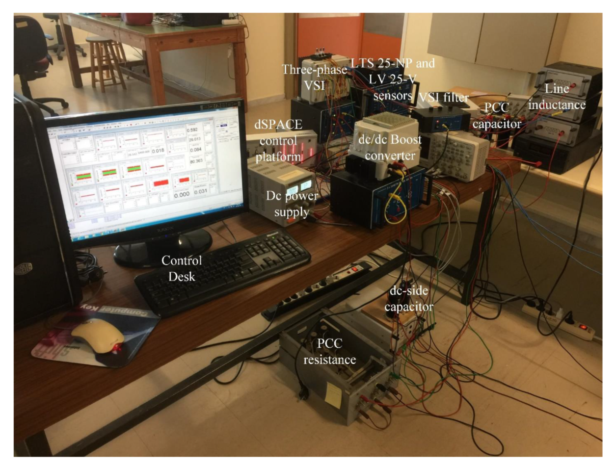
In order to further evaluate the performance of the system under the action of the deployed closed-loop control scheme, an experimental procedure is also established based on the complete system of Figure 1. In particular, the experimental setup comprises a dc/dc boost converter representing a DER current source feeding a three-phase VSI. The VSI is connected through an RL filter to the PCC, which in turn is connected to the grid via an RL line. The setup as developed in the laboratory environment is illustrated in Figure 3.

The proposed control scheme is implemented using a dSPACE DS1104 platform [38], which is an ideal solution for fast and accurate prototyping of control designs. This particular system is based on a processor board, featuring a PowerPc 603e floating-point processor running at 250 MHz, slave-DSP system, several I/O ports, along with A/D and D/A channels. Furthermore, the real-time interface (RTI) [39] for dSPACE systems provides the capability of directly linking MATLAB-Simulink control models to the DS1104 hardware, by generating and compiling real-time code. All the required analog measurements, i.e., voltages and currents, are provided to the A/D converter ports of the dSPACE board by using LV-25V voltage and LEM LTS 25-NP current sensors. The controller then suitably generates both a pulse-width-modulated signal of 5 kHz and a sinusoidal-pulse-width-modulated signal of 10 kHz, which are provided to the driving circuits of the dc/dc boost converter and the three-phase VSI, respectively.

The experimental setup parameters are listed in

Table 1. System parameters.

Parameter	Quantity	Value
$R_f$	Resistance of the VSI filter	7.5 Ω
$L_f$	Inductance of the VSI filter	1 mH
$C_{dc}$	DC-side capacitance	100 μF
$C_B$	Capacitance at the PCC	2200 μF
$R_B$	Resistance at the PCC	1200 Ω
$R_{Line}$	Line resistance	6.4 Ω
$L_{Line}$	Line inductance	5 mH
$\left|V_G\right|$	Grid Voltage Magnitude	25 V
$f$	Power grid frequency	50 Hz

. The controller gains are selected as ${\overline{k}}_{Pd}={\overline{k}}_{Pq}=320$ and ${\overline{k}}_{Id}={\overline{k}}_{Iq}=16,000$. Also, it is chosen ${\overline{k}}_{If}={\overline{k}}_{Ig}=2$, while the outer-loop controllers gains are selected to be: $k_{Pdc}=0.064$, $k_{Idc}=0.352$ and $k_{PV}=0.001$, $k_{IV}=0.01$. The dc and ac voltage reference values are set at $V_{dc}^{ref}=80 \mathrm{V}$ and $V_{dqB}^{ref}=25 \mathrm{V}$, respectively.

4. Results and Discussion

Based on the aforementioned analysis and the system parameters given in the previous Section, extensive simulations are conducted and presented in the following Section 4.1. In particular, comparisons are made between the simulated results with the mean value model of the VSI and the results obtained via the accurate switching model. In Section 4.2, the experimental setup previously described is used to provide real-time results.

4.1. Simulation Results

Various changes of the external inputs have been considered, namely, rapid changes of the DER output current, at times t = 1, 2 and 3 s. Figure 4 and Figure 5 depict the q- and d-axis VSI output current component, respectively. Their response is fairly fast as they reach steady-state without significant overshoots or long transients.

In Figure 6 and Figure 7, one can see the fast and effective ac- and dc-voltage regulation on the weak ac-grid and the dc-side, respectively. As expected, a small difference is observed in the dynamic response of the system between the mean-value and the accurate model. It is also noticed that the mean value model used for the VSI is closer to the real model as the switching frequency increases.

Finally, Figure 8 shows the active and reactive power injected to the grid at the PCC. One can easily notice that the power transferred exactly follows the changes of the DER output current. This is, in fact, one of the main advantages of the applied control design, i.e., its capability to transfer the total power produced while it maintains the ac voltage constant.

In general, the implemented control design leads the system efficiently to the steady state in a stable and precise manner. Both the mean value model and the accurate one, fully verify the effectiveness of the proposed control scheme to respond in rapid changes with fast and smooth action, featuring only small overshoots and very limited transient periods.

4.2. Experimental Results

Two experimental cases have been considered.

In Experiment 1, a step-change of the DER current source occurs, at approximately $t_1=6 \mathrm{s}$ and $t_2=10$. Figure 9, Figure 10, Figure 11 and Figure 12 represent the system response.

In Figure 9 and Figure 10, the q- and d- current components are shown, while in Figure 11 and Figure 12, the dc and ac voltage responses are depicted. It can easily be seen that the current follows the command input changes, while both the dc- and ac-voltages remain at the desired value. Only limited transients are observed during the external input changes, indicating that the proposed control scheme effectively retains the steady-state operation.

The ripple appeared in both the current and voltage responses are in acceptable bounds around their expected mean values, a fact also observed in the simulation results presented in Section 4.1 for the cases where the accurate switching power electronic models have been used.

In Experiment 2, a grid-originated voltage disturbance is studied. In particular, a sudden grid-side voltage drop is introduced at approximately t = 7 s into the experiment. The main aim is to evaluate the outer-loop ac voltage controllers’ performance in terms of effectively regulating the PCC voltage at the desired steady-state value and the PLLs capability to maintain synchronism with the utility.

Figure 13 and Figure 14 represent the dc voltage response and the ac voltage magnitude response at the PCC, respectively. In both figures one can observe that the voltages return to their reference value after a fast, transient period. It is clear that the PLL operation is very satisfactory at keeping the system in synchronism, while the dual loop controllers effectively compensate the phenomenon.

Finally, by examining the results of both the experimental cases, it is easily realized that the stability and robustness of the system are fully validated and are absolutely in compliance with the results derived from the simulation.

5. Open Questions and Perspectives

Motivated by the transition of power systems towards increased RES integration, a lot of open questions are raised.

In the frame of the present work, a first interesting open issue is how the proposed decentralized control scheme and stability analysis approach can be generalized and applied to larger multi-converter ac power systems. This further research could provide a common formulation of control design and analysis for large-scale power systems considering the interaction of different dynamics (converter dynamics, inner-loop controller, synchronization dynamics, line dynamics) and quantifying the parameters (e.g., set-points, control gains, transmission line parameters, etc.) for which stability for the overall system can be ensured. This formulation would be a very important tool for the efficient, reliable and stable operation of modern DG-based power grids.

In future research works, another interesting question is how this design can be combined with upper networked layers of management and control schemes. This constitutes a significant step that incorporates the primary level control and stability analysis into the general power system management and planning, based on market and consumer constraints and needs. Such an extension combines and integrates the overall power system performance with the technical possibilities and all the new issues imposed by a smart grid operation, which is expected to become very important in the near future.

6. Conclusions

In this paper, the challenging issue of efficiently controlling the VSI interface used to connect a DER to a weak ac grid is considered. Thus, in the present work, the main concept is based on the fact that the VSI enables us to provide decentralized and remote power control. To implement this concept, the system was integrated by each entire model in order to be exploited as a control asset capable to compensate the power system weakness in long-distance areas. Since the grid strength has a significant impact on the overall system operation and particularly to the ac-voltage magnitude at the connection point, the controller tasks concentrated on the ac- and dc-side voltage regulation of the VSI. Particularly, a novel, PLL-driven cascaded control scheme was proposed and analyzed in detail by an extensive theoretical analysis. In both the PLL and the controller designs, significant innovations were introduced aiming to trade-off the system performance between the necessity of obtaining control schemes independent from the system parameters and the strict obligation of guaranteeing stability. Finally, simulation and experimental results were presented, in order to evaluate the entire system performance under varying operating conditions and to further verify the theoretical claims in the case studied. All the results indicate a fully satisfactory response and successful operation. Overall, the proposed control scheme and analysis aims to help accelerate the integration of RES into energy systems, improve the operation of the electrical grid and enhance the security and stability of power systems.

References

1. EU Climate Action: Climate Strategies & Targets: 2030 Climate & Energy Framework. Available online: https://ec.europa.eu/clima/policies/strategies/2030_en (accessed on 2 March 2020).
2. Transforming Our World: The 2030 Agenda for Sustainable Development. Available online: https://sustainabledevelopment.un.org/post2015/transformingourworld (accessed on 2 March 2020).
3. Blaabjerg, F.; Chen, Z.; Kjaer, S.B. Power electronics as efficient interface in dispersed power generation systems. IEEE Trans. Power Electron. 2004, 19, 1184–1194. [Google Scholar] [CrossRef]
4. Vasquez, J.C.; Guerrero, J.M.; Savaghebi, M.; Eloy-Garcia, J.; Teodorescu, R. Modeling, analysis, and design of stationary-reference-frame droop-controlled parallel three-phase voltage source inverters. IEEE Trans. Ind. Electron. 2013, 60, 1271–1280. [Google Scholar] [CrossRef] [Green Version]
5. Hossain, M.A.; Pota, H.R.; Issa, W.; Hossain, M.J. Overview of AC Microgrid Controls with Inverter-Interfaced Generations. Energies 2017, 10, 1300. [Google Scholar] [CrossRef]
6. Yazdani, A.; Iravani, R. Voltage-Sourced Converters in Power Systems; Wiley Press: Hoboken, NJ, USA, 2010. [Google Scholar]
7. Zhang, L.; Harnefors, L.; Nee, H. Interconnection of Two Very Weak AC Systems by VSC-HVDC Links Using Power-Synchronization Control. IEEE Trans. Power Syst. 2011, 26, 344–355. [Google Scholar] [CrossRef]
8. Diedrichs, V.; Beekmann, A.; Busker, K. Control of Wind Power Plants Utilizing Voltage Source Converter in High Impedance Grids. In Proceedings of the 2012 IEEE Power and Society General Meeting, San Diego, CA, USA, 22–26 July 2012; pp. 1–9. [Google Scholar]
9. Huang, Y.; Yuan, X.; Hu, J.; Zhou, P. Modeling of VSC Connected to Weak Grid for Stability Analysis of DC-Link Voltage Control. IEEE J. Emerg. Sel. Top. Power Electron. 2015, 3, 1193–1204. [Google Scholar] [CrossRef]
10. Mao, M.; Hu, J.; Chang, L. Voltage stability analysis on wind generation system from current control time-scale. In Proceedings of the Chinese Automation Congress (CAC), Jinan, China, 20–22 October 2017; pp. 7010–7015. [Google Scholar]
11. Li, X.; Lin, H. Stability Analysis of Grid-Connected Converters with Different Implementations of Adaptive PR Controllers under Weak Grid Conditions. Energies 2018, 11, 2004. [Google Scholar] [CrossRef] [Green Version]
12. Li, M.; Zhang, X.; Zhao, W. A Novel Stability Improvement Strategy for a Multi-Inverter System in a Weak Grid Utilizing Dual-Mode Control. Energies 2018, 11, 2144. [Google Scholar] [CrossRef] [Green Version]
13. Din, Z.; Zhang, J.; Bassi, H.; Rawa, M.; Song, Y. Impact of Phase Locked Loop with Different Types and Control Dynamics on Resonance of DFIG System. Energies 2020, 13, 1039. [Google Scholar] [CrossRef] [Green Version]
14. Yang, H.; Yuan, X. Modeling and Analyzing the Effect of Frequency Variation on Weak Grid-Connected VSC System Stability in DC Voltage Control Timescale. Energies 2019, 12, 4458. [Google Scholar] [CrossRef] [Green Version]
15. Wang, D.; Huang, Y.; Liao, M.; Zhu, G.; Deng, X. Grid-Synchronization Stability Analysis for Multi DFIGs Connected in Parallel to Weak AC Grids. Energies 2019, 12, 4361. [Google Scholar] [CrossRef] [Green Version]
16. Longhi, L.G.S.; Secchi, A.R.; Trierweiler, J.O.; Lima, E.L. A Possible Approach to Solve Nonlinear H-Infinity Control Problem. Proc. IFAC 2000, 33, 887–892. [Google Scholar] [CrossRef]
17. Sedhom, B.E.; Hatata, A.Y.; El-Saadawi, M.M.; Abd-Raboh, E.E. Robust adaptive H-infinity based controller for islanded microgrid supplying non-linear and unbalanced loads. IET Smart Grid 2019, 2, 420–435. [Google Scholar] [CrossRef]
18. Kushwaha, S.K.S.; Mohanty, S.R.; Samuel, P. Non-linear H-infinity Control for Grid-interactive Offshore Wind Farm and Marine Current Farm. In Proceedings of the 2nd IEEE International Conference on Power Electronics, Intelligent Control and Energy Systems (ICPEICES), Delhi, India, 22–24 October 2018; pp. 420–425. [Google Scholar]
19. Guo, C.; Liu, W.; Zhao, C.; Iravani, R. A Frequency-Based Synchronization Approach for the VSC-HVDC Station Connected to a Weak AC Grid. IEEE Trans. Power Deliv. 2017, 32, 1460–1470. [Google Scholar] [CrossRef]
20. Wu, B.; Lang, Y.; Zargari, N.; Kouro, S. Power Conversion and Control of Wind Energy Systems; Wiley Press: Hoboken, NJ, USA, 2011. [Google Scholar]
21. Makrygiorgou, D.I.; Alexandridis, A.T. Stability Analysis of DC Distribution Systems with Droop-Based Charge Sharing on Storage Devices. Energies 2017, 10, 433. [Google Scholar] [CrossRef] [Green Version]
22. Krein, P.T.; Bentsman, J.; Bass, R.M.; Lesieutre, B.L. On the Use of Averaging for the Analysis of Power Electronic Systems. IEEE Trans. Power Electron. 1990, 5, 182–190. [Google Scholar] [CrossRef]
23. Haugen, F. Basic Dynamics and Control; TechTeach: Skien, Norway, 2010; ISBN 978-82-91748. [Google Scholar]
24. Papageorgiou, P.C.; Alexandridis, A.T. Innovations on the control of VSC-based dc-links connecting distributed generation to the grid. In Proceedings of the IECON 2019 45th Annual Conference of the IEEE Industrial Electronics Society, Lisbon, Portugal, 14–17 October 2019; pp. 3919–3924. [Google Scholar]
25. Papageorgiou, P.C.; Alexandridis, A.T. Stabilizing the VSI response in microgrids via novel PI controllers. proceedings of the 2017 International Symposium on Power Electronics (Ee), Novi Sad, Serbia, 19–21 October 2017; pp. 1–6. [Google Scholar]
26. Krommydas, K.F.; Alexandridis, A.T. Dynamic Analysis of PLL-Synchronized Power Inverter Interface for Grid-Connected PV Systems. In Proceedings of the 2018 Annual American Control Conference (ACC), Milwaukee, WI, USA, 27–29 June 2018; pp. 2127–2132. [Google Scholar]
27. Papageorgiou, P.C.; Alexandridis, A.T. A suitable to the microgrid analysis approach for nonlinear modeling and control of an inverter interface. In Proceedings of the 25th Mediterranean Conference on Control and Automation (MED-2017), Valletta, Malta, 3–6 July 2017; pp. 522–527. [Google Scholar]
28. He, X.; Geng, H.; Ma, S. Transient stability analysis of grid-tied converters considering PLL’s nonlinearity. Cpss Trans. Power Electron. Appl. 2019, 4, 40–49. [Google Scholar] [CrossRef]
29. Sira-Ramirez, H.; Silva-Ortigoza, R. Control Design Techniques in Power Electronics Devices; Springer: London, UK, 2006. [Google Scholar]
30. Sontag, E.D. Input to state stability: Basic concepts and results. In Nonlinear and Optimal Control Theory. Lecture Notes in Mathematics, 1st ed.; Nistri, P., Stefani, G., Eds.; Springer: Berlin, Germany, 2008; Volume 1932, pp. 163–220. [Google Scholar]
31. Khalil, H.K. Nonlinear Systems, 3rd ed.; Prentice-Hall: Upper Saddle River, NJ, USA, 2002. [Google Scholar]
32. Konstantopoulos, G.C.; Alexandridis, A.T. Generalized Nonlinear Stabilizing Controllers for Hamiltonian Passive Systems with Switching Devices. IEEE Trans. Control Syst. Technol. 2013, 21, 1479–1488. [Google Scholar] [CrossRef]
33. Alexandridis, A.T. Studying State Convergence of Input-to-State Stable Systems with Applications to Power System Analysis. Energies 2020, 13, 92. [Google Scholar] [CrossRef] [Green Version]
34. Aström, K.J.; Hägglund, T. PID Controllers: Theory, Design, and Tuning, 2nd ed.; International Society of Automation: Research Triangle Park, NC, USA, 1995. [Google Scholar]
35. Fitri, I.R.; Kim, J.-S.; Song, H. A Robust Suboptimal Current Control of an Interlink Converter for a Hybrid AC/DC Microgrid. Energies 2018, 11, 1382. [Google Scholar] [CrossRef] [Green Version]
36. Yan, Q.; Tasiu, I.A.; Chen, H.; Zhang, Y.; Wu, S.; Liu, Z. Design and Hardware-in-the-Loop Implementation of Fuzzy-Based Proportional-Integral Control for the Traction Line-Side Converter of a High-Speed Train. Energies 2019, 12, 4094. [Google Scholar] [CrossRef] [Green Version]
37. Haugen, F. Comparing PI Tuning Methods in a RealBenchmark Temperature Control System. Modeling Identif. Control 2010, 31, 79–91. [Google Scholar] [CrossRef]
38. dSPACE GmbH. DS1104 R&D Controller Board; USA and Canada dSPACE Inc.: Wixom, MI, USA, 2011. [Google Scholar]
39. dSPACE GmbH. Real-time interface (RTI and RTI-MP), dSPACE Implementation Guide 5.2; USA and Canada dSPACE Inc.: Wixom, MI, USA, 2005. [Google Scholar]
Figure 1. Overall power and control block diagram of the system under consideration.
Energies 13 01373 g001
Figure 2. The PLL synchronization process.
Energies 13 01373 g002
Figure 3. Experimental setup of the considered system.
Energies 13 01373 g003
Figure 4. The VSI output q-axis current component.
Energies 13 01373 g004
Figure 5. The VSI output d-axis current component.
Energies 13 01373 g005
Figure 6. The dc-side voltage response.
Energies 13 01373 g006
Figure 7. Voltage magnitude response at the PCC.
Energies 13 01373 g007
Figure 8. Active and Reactive Power injected to the grid.
Energies 13 01373 g008
Figure 9. The VSI output q-axis current component (Experiment 1).
Energies 13 01373 g009
Figure 10. The VSI output d-axis current component (Experiment 1).
Energies 13 01373 g010
Figure 11. The dc-side voltage response (Experiment 1).
Energies 13 01373 g011
Figure 12. PCC voltage magnitude (Experiment 1).
Energies 13 01373 g012
Figure 13. The dc-side voltage response (Experiment 2).
Energies 13 01373 g013
Figure 14. Voltage magnitude response at the PCC (Experiment 2).
Energies 13 01373 g014