Abstract
The modern distribution networks under the smart grid paradigm have been considered both interconnected and reliable. In grid modernization concepts, the optimal asset optimization across a certain planning horizon is of core importance. Modern planning problems are more inclined towards a feasible solution amongst conflicting criteria. In this paper, an integrated decision-making planning (IDMP) approach is proposed. The proposed methodology includes voltage stability assessment indices linked with loss minimization condition-based approach, and is integrated with different multi-criteria decision-making methodologies (MCDM), followed by unanimous decision making (UDM). The proposed IDMP approach aims at optimal assets sitting and sizing in a meshed distribution network to find a trade-off solution with various asset types across normal and load growth horizons. An initial evaluation is carried out with assets such as distributed generation (DG), photovoltaic (PV)-based renewable DG, and distributed static compensator (D-STATCOM) units. The solutions for various cases of asset optimization and respective alternatives focusing on technical only, economic only, and techno-economic objectives across the planning horizon have been evaluated. Later, various prominent MCDM methodologies are applied to find a trade-off solution across different cases and scenarios of assets optimization. Finally, UDM is applied to find trade-off solutions amongst various MCDM methodologies across normal and load growth levels. The proposed approach is carried out across a 33-bus meshed configured distribution network. Findings from the proposed IDMP approach are compared with available works reported in the literature. The numerical results achieved have validated the effectiveness of the proposed planning approach in terms of better performance and an effective trade-off solution across various asset types.
1. Introduction
The global load demand for electricity has increased significantly, pushing the distribution network (DN) to their operational limits results in issues i.e., voltage stability and system losses. Also, the distribution grid is more susceptible to technical, cost-economic, environmental, and social issues, especially from the perspective of meeting growing demand [1]. Conventionally, the traditional distribution grid paradigm was deterministically designed and planned to retain unidirectional power flow under radial topology, particularly considering simple protection schemes and easy control. Moreover, the traditional planning tools usually applied for distribution network planning problems (DNPP) might not remain feasible to mitigate the concerned issues by replication the existing infrastructure, which is certainly not a cost-effective solution [2]. The DNPP needs the support of various optimization tools of different genres aiming for futuristic scenarios.
Practically, DNPP aims realistically towards achieving a trade-off solution under multiple conflicting criteria subjected to various non-linear system constraints. The topology constraint in most of the DNPP studies has considered radial topology rather than interconnected configuration [3]. Similarly, distributed generation (DG) incorporation was neither considered in the planning stage nor assisted in the operational stage of the radial-structured distribution network (RDN) in the traditional grid paradigm. However, the addition of DG in DN has transformed the passive nature of the system into an active one and hence also transformed into an active distribution network (ADN) [4]. The RDN along with optimal DG placement (ODGP) can either remain in reconfigured configuration or be transformed into interconnected topologies i.e., loop DN (LDN) or mesh DN (MDN) on the basis of changing the state of normally open (NO) and tie-switches (TS). The interconnected arrangement is more suitable for densely inhabited urban centers and is feasible due to the cost-effectiveness of existing infrastructure employment [5,6].
In the recent literature studies, DNPP considering asset optimization has been considered as one of the core research dimensions to strengthen DN with various types of objectives subjected to constraints, with various methods applied at various system models. Plenty of techniques and methodologies of the different genres have been proposed for assets optimization studies (predominately DG) aiming at various single and multiple objectives (or criteria), which are usually conflicting in nature, under numerous constraints [7,8,9,10]. Among the main efforts to solve the aforementioned planning problems, the DN planners and utility operators consider optimal assets placement, dominated by DG units, in distribution mechanisms on the basis of size, location, quantity, capacity, type, and topology. The most sorted out solutions include cost-economic, technical, and environmental benefits, aiming at the achievement of trade-off solutions among multiple objectives [11]. The DNPP with DGs and associated assets have been considered a worthy solution, particularly enabling utilities to improve power quality and inducing deferral in DN up-gradation during load growth across the planning horizon, which usually spread across one year to several [12].
The methods addressing ODGP problems have been accredited to various objectives, primarily from the viewpoint of voltage (profile) maximization (VM) and system loss minimizations (LM). Moreover, technical advantages include DG penetration in DN, power quality (at utilities and consumers end), system stability, reliability, improved (bidirectional) power flows, and short-circuit-current (SCC) levels [7,8]. The other associated objectives concerned include the cost of active/reactive power losses, initial capital, operational, maintenance, and running cost. The environmentally feasible solutions with social acceptability concerning technology acceptance and consumer comfort are also amongst the addressed goals [9,10,11]. Besides DG, assets like reactive power compensation devices are also utilized for optimal operation of the DNPP, such as capacitors and flexible ac transmission system (FACTS) devices [6,12,13]. Furthermore, the application of distributed static compensators (D-STATCOMs) with DGs have been mostly reviewed in RDN [14]. In addition, normally open tie-switches (TS), normally closed sectionalize switches, concerned conductor replacements, and substation capacity enhancements are considered in asset optimization in DN. Furthermore, reconfiguration of a network to modified radial or to an interconnected topology has also been considered as a key component in the asset optimization of DN, from the viewpoint of DNPP [15,16].
In all of the above-mentioned works [6,7,8,9,10,11,12,13,14,15,16], the assets mostly used are DG, reactive power compensating devices, grid reinforcement with associated devices, and change of DN topology. The most significant asset optimization approaches aiming at optimal sitting and sizing under system constraints include classical techniques like analytical, deterministic, numerical, and exhaustive search. The heuristic, meta-heuristic, artificial intelligence-based algorithms include nature-, society-, or population-inspired methodologies. However, these algorithms can result in local optima in various cases. This particular limitation is usually bridged with hybrid algorithms aiming at global optima. Besides that, multi-criteria (also known as multi-attribute) decision-making (MCDM) techniques are employed to sort out a trade-off solution among various concerned criteria/objectives of contradictory nature. Such methods can be priori optimized with assigning weights (subjectively or objectively) to each criterion (priori methods) or applied later (posteri methods) on a various number of solutions obtained from inner optimization. Besides that, commercial solvers are also employed for planning purposes such as the general algebraic modeling system (GAMS) [15,16].
From the perspective of DN, consideration of radiality constraint has dominated in most of the above-mentioned reviewed works, aiming at ODGP. However, the interconnected DN such as LDN and MDN are not as prevalent as their radial counterparts and need consideration from the viewpoint of planning [17]. LDN and MDN have been assessed from the perspective of various analytical/numerical and hybrid techniques from the perspective of various types of objectives such as loss minimization (LM) [18,19,20], voltage stabilization (VS) [19,20], DG penetration [19,20], reliability, and cost-related indices [20,21]. The LDN/MD-based infrastructure optimization has considered various assets such as the number of TS [22,23] and its influence on different load levels and evaluation across load growth [20,24,25]. Moreover, the replacement of TS with fault current limiter (FCL) [26], reinforcement versus looping/meshing [27,28], and optimal utilization of D-STATCOMs only in interconnected DN have also been considered [29]. In the recent works reported in [30,31], two different variants of an integrated planning approach incorporating improved voltage stability assessment indices (VSAI) along with loss minimization condition (LMC) have been employed for optimal asset optimization in MDN such as DG only and DG with D-STATCOM for VS, LM, and cost-related objectives under normal load.
The optimal planning of D-STATCOM is accredited with increasing penetration of renewable generation (REG)-based DGs, VS, LM, and minimizing associated cost objectives. Like most of the ODGP-based DNPP, D-STATCOM integration has mostly been considered radiality constraint [14]. It is also found that D-STATCOM has been utilized in mostly RDN for the achievement of core objectives such as system losses reduction, voltage curve improvement, and reduction of concerned costs. The work in [32] was aimed towards cost reduction along with the attainment of technical objectives. The D-STATCOM on the basis of asset placement on the same or different buses along with DGs or separately have been reported in [33,34,35], supported by relevant technical performance evaluations. The D-STATCOM placement on different load levels [36] and multiple asset sets (DG and D-STATCOM) on different buses [29,30,31,32,33,34] and the same buses [37] have been evaluated from various objectives. It is also important to mention that the works reported in [14,32,33,34,35,36,37] have mostly aimed at RDN, centered on a single branch (two buses) model and cannot encompass the core dynamic of LDN and MDN that is usually fed by more than on sending end.
From the viewpoint of MCDM, hybrid methodologies have been put forward to achieve multiple objectives or evaluation under various criteria. In the research works [38,39,40,41], the prominent MCDM methods employed are weighted sum method (WSM), weighted product method (WPM), technique for order preference by similarity to ideal solution (TOPSIS), preference ranking organization method for enrichment of evaluations (PROMETHEE), and RDN is reconfigured in terms of asset optimization to achieve objects such as active power losses, reliability, and average energy not served (AENS). Also, the heuristic and meta-heuristic methods in combination with MCDM have been utilized in various asset planning works to achieve a suitable solution. In [42], genetic algorithm (GA) and TOPSIS have been employed for optimal sitting and sizing of DG and remote terminal units (RTUs). In [43], DN is radially reconfigured with non-dominated GA-II (NSGA-II) and a combination of MCDM techniques to achieve an optimal solution with fewer energy losses, an optimum level of energy not served (ENS), and load balancing, respectively.
The particle swarm optimization (PSO) along with the analytical hierarchal process (AHP) in [44] have been utilized to achieve multi-objective solutions across technical, environmental, and economic-based criteria, with DGs in radially reconfigured DN. In [45], teaching–learning-based optimization is employed for multi-objectivity using penalty factors for a DG-only solution and an improved variant in [46] is used to achieve a solution under multiple assets (DGs and capacitors). The multi-objective, opposition-based, chaotic differential Equation-based method in [47] is used for techno-economic analysis of only DGs and to avoid premature convergence in the above-mentioned meta-heuristic methods. The research works in [48,49] have considered DG and renewable DG (REG) penetration along with various indices to offer a simple solution aiming at voltage stability and loss minimizations. The load growth has been briefly discussed for DGs only from the viewpoint of technical objectives considering MCDM in [50] and voltage stability index with MCDM-based methodology in LDN in [51,52].
As aforementioned, RDN was not planned to integrate DGs and nearly every DNPP with any sort of asset is aimed credibly towards achieving multiple conflicting objectives under any topology, abiding nonlinear system constraints. Thus, the modernization of DS in planning and operation with several DGs types and transformations to an ADN has become a noticeable research dimension. Hence, DN modernization with efficient asset optimization and interconnected topology can be considered as a prominent research dimension in the area of the smart distribution network (SDN) under the smart grid (SG) paradigm from the perspective of planning, scheduling, and operation, respectively. Moreover, the SDN under the SG paradigm is expected to be reliable from interconnected topology and multi-criteria attainment oriented with conflicting nature. The planning tools also need to be updated and evaluated across load growth considering multi-dimensional evaluation, since technically efficient solution might not be cost-effective. Hence, a composite asset planning problem with multi-criteria optimization needs research consideration, supported with multi-dimensional performance evaluation across load growth. Although reviewed works have partially addressed the aforementioned issues from various perspectives, bridging the limitations offered in reviewed literature is the motivating force for research and serves as the impetus of this paper.
In this paper, VSAI interrelated with LMC-based approach is integrated with various MCDM methodologies, followed by unanimous decision making (UDM), and is given the name integrated decision-making planning (IDMP). The MCDM methodologies employed in IDMP include WSM, WPM, TOPSIS, and PROMETHEE. The proposed IDMP approach aims at bridging the research gap in the reviewed literature by optimal asset optimizations in MDN for a trade-off solution amongst various alternatives across normal and load growth horizons. The 33-bus distribution system is configured to MDN as the precedence of ADN unlike their radial counterparts. The VSAI indices used in this approach are specifically designed and based on the multi-branch model and encompass the dynamics of an interconnected DN i.e., MDN, unlike radial counterparts based on a single branch model. The assets involved in IDMP have DG operating at various lagging power factors (LPF) contributing both active and reactive power, and renewable DG such as photovoltaic (PV) system contributes active power only and D-STATCOM units providing reactive power only. The approach provides alternatives across various axis such as technical only, economic only, and techno-economic objectives across the planning horizon. The MCDM methodologies provide a wide range of alternatives as solutions. In addition, unanimous decision making (UDM) across various MCDM methodologies in terms of their respective scores are offered. Moreover, the proposed IDMP approach can serve as a tool for future planning of interconnected ADN, particularly supporting planning engineers and researchers from the perspective of the SG paradigm. The main contributions of the proposed work are as follows.
- (i)
- Integrated decision-making planning approach (IDMP) for optimal asset optimization.
- (ii)
- Evaluation of the offered approach under various multiple assets (sitting and sizing) with LPF.
- (iii)
- Evaluation of offered approach under various techno-economic performance metrics.
- (iv)
- Detailed evaluation of alternatives across normal load and load growth horizons.
- (v)
- Detailed evaluation of alternatives across four MCDM methodologies.
- (vi)
- Offering a unanimous decision making (UDM) score as per rank of alternatives.
- (vii)
- Numerical evaluations of the proposed approach on 33-Bus test DN.
- (viii)
- Validations of achieved results with the findings reported in the available literature.
This paper is organized in the following sections. Section 2 offers the proposed IDMP approach along with concerned mathematical expressions. Section 3 offers a computation procedure for the IDMP approach, setup for simulations, and performance evaluation indicators. In Section 4, the attained numerical results regarding the effectiveness of the proposed approach is evaluated with multiple DG operating at various LPF, REG, and D-STATCOM sets, on the basis of optimal assets sitting and sizing perspective, evaluated under various performance metrics, demonstrated on 33-bus test MDN. The MCDM evaluations followed by UDM scores amongst various alternatives are presented in this section. The comparison of the proposed IDMP approach with existing research work is validated by comparison with existing works in Section 5. The paper concludes in Section 6.
2. Proposed Integrated Decision-Making Planning Approach
2.1. Voltage Stability Assessment Index_A (VSAI_A) for Mesh Distribution Network
The electrical equivalent MDN model in Figure 1 consists of three branches that represent DN feeders and two tie-line (TL) for in between linkage. The TS are closed to convert the DN into MDN. The voltages from sending end buses/nodes (n1b, n3b and n5b) have been considered to exhibit the same magnitude and phase angle (δ), and is represented as one source node n1b, respectively. The receiving end buses/nodes (n2b, n4b, and n6b) are connected via two TB (with insignificant impedance) via respective TS. Also, the loads S2b, S4b, and S6b, at n2b, n4b, and n6b are considered as lumped load at bus/node m2b with a voltage magnitude of V2b, as shown in Figure 1, respectively.
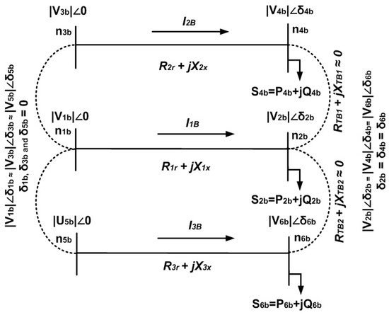
Figure 1.
Electrical equivalent diagram of mesh distribution network [30,31].
In this paper, two of the VSAI indices formulated and reported in our previous publications [30,31] have been employed along with LMC aiming at pinpointing possible alternatives in terms of asset sitting as sizing with various decision variables. Later, various MCDM techniques are further applied for sorting out the best alternatives amongst available solutions. The VSAI reported in [30] is designated as VSAI_A and the other one reported in [31] is designated as VSAI_B, aiming at an optimal sitting of the asset. The procedure of LMC remains the same in both VSAIs as per their integrated planning approach. The VSAI_A along with feasible solution V_A are shown in Equations (1) and (2), where the variables are separately shown in Equations (3)–(6). The threshold value of VSAI_A value is between 0 (instability) and 1 (stable).
where
2.2. Voltage Stability Assessment Index_B (VSAI_B) for Mesh Distribution Network
The expression for VSAI_B is illustrated in Equation (7) and it is considered that unlike VSAI_A under normal conditions, the numerical value of VSAI_B is close to zero. During unstable conditions, the expression exceeds the numerical threshold of 1. The expression for VSAI_B and its feasible solution V_B are shown in Equations (7) and (8) with respective variables shown separately in Equations (9)–(10), respectively.
where
2.3. Loss Minimization Condition (LMC) for Mesh Distribution Network
The LMC for VSAI_A and VSAI_B is the same at its optimal sizing of an asset at which the loop current across the tie-line is zero [30,31]. Figure 2 shows the electrical equivalent model of an equivalent MDN aiming at LMC. The loading at bus m2b is considered at a normal load S2b, fed by two TS ends (n4b and n6b) via tie-line currents (ITB1 and ITB2), besides dedicated serving source (n1b), respectively. The optimal sizing of assets that reduces ITB1 and ITB2 to zero indicates the optimal sizing of the respective asset. The LMC relations for base cases shown for apparent power (LMC_S) is shown in Equation (11). The optimal asset size at which ILP1 and ILP2 are zero represents the best case at which both active (P) and reactive (Q) power losses are minimized and indicated as the LMC_P and LMC_Q in Equation (12), respectively [30,31].
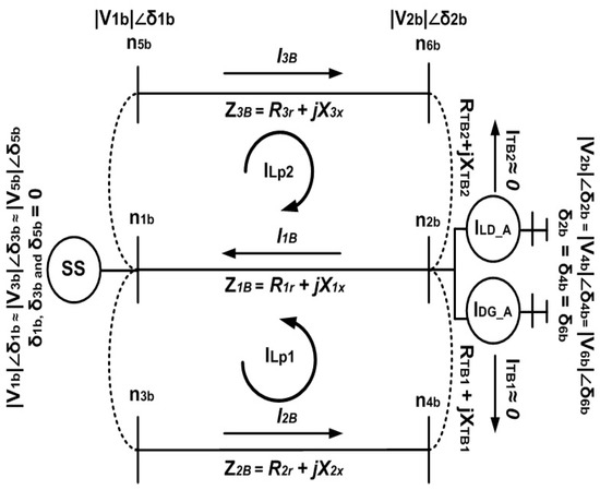
Figure 2.
Equivalent mesh distribution network (MDN) model with tie and loop currents reduction aiming at loss minimization condition (LMC) [30,31].
2.4. Decision-Making (DM) Methodologies
The decision-making (DM) problems addressing multiple-attributes can be broadly classified among two types of classifications [38,41]. In the first type, referred to as the priori methods, weights are assigned (subjectively or objectively) to each criterion in case of predetermined solutions (also called alternatives). Such a method is also referred to as multi-attribute or multi-criteria decision-making. The second type refers to the posteri methods-based applications in which several solutions are initially obtained from inner optimization and, later, a best trade-off solution is acquired with any second-stage DM methodology. The methodologies related to this class have been utilized in the proposed IDMP approach. The generic decision matrix in MCDM is shown in Table 1.

Table 1.
Generic decision matrix in multiple attribute decision-making (MCDM) methodologies.
2.4.1. Weighted Sum Method (WSM)
The WSM is amongst the most used techniques for calculating the rank aiming at the achievement of the best solution among multiple solutions (also called alternatives) in terms of the highest score. For that purpose, the following equation finds the highest score solution as the optimum one considering m alternatives evaluated across n criteria.
where i = 1,2, … m, indicates the weighted sum score, is the normalized score of i-th alternative/solution from the reference of j-th criterion and is the weight associated with j-th criterion. Later on, the consequential cardinal scores for every alternative/solution can be utilized to rank or choose the best alternative. As aforementioned, the solution with the maximum score is considered as the best alternative amongst rest.
2.4.2. Weighted Product Method (WPM)
The WPM compares alternatives Akj and Alj across n criteria and the optimal solution is obtained by multiplication aiming at calculating ranks of alternatives rather than addition, as shown in WSM. The optimum solution in a pairwise comparison is the one that exhibits the highest score as shown in the Equation below.
where i = 1,2, … m, as previously, is the normalized score of the i-th alternative from the reference of j-th criterion and is the weight associated with j-th criterion.
2.4.3. Technique for Order Preference by Similarity to Ideal Solution (TOPSIS)
After defining n criteria and m alternatives, the normalized decision matrix is established. The normalized value is calculated from Equation (15), where is the i-th criterion value for alternative Aj (j = 1… m and i = 1, …, n).
The normalized weighted values in the decision matrix are calculated as per Equation (16):
The positive ideal and negative ideal solution are derived as shown below, where and are related to the benefit and cost criteria (positive and negative variables), as shown in Equation (17) as follows.
From the n-dimensional Euclidean distance, is calculated in the given equation as the separation of every alternative from the ideal solution. The separation from the negative ideal solution is shown in a relationship indicated in Equation (18).
The relative closeness to the ideal solution of each alternative is calculated from Equation (19):
After sorting the values, the maximum value corresponds to the best solution to the problem.
2.4.4. Preference Ranking Organization Method for Enrichment of Evaluations-II (PROMETHEE-II)
The procedure of PROMETHEE II is indicated as follows.
Step 1: Normalize the decision matrix using the following Equation:
where is the performance measure of i-th alternative with respect to j-th criterion. For non-beneficial criteria, Equation (20) can be rewritten as follows:
Step 2: Calculate the evaluative differences of i-th alternative with respect to other alternatives. This step involves the calculation of differences in criteria values between different alternatives pairwise.
Step 3: Calculate the preference function,
Step 4: Calculate the aggregated preference function taking into account the criteria weights. The aggregated preference function is shown in Equation (23) as follows, where is the relative importance (weight) of j-th criterion is.
Step 5: Determine the leaving and entering outranking flows, such as the leaving (or positive) flow for i-th alternative as indicated in Equation (23) and entering (or negative) flow for i-th alternative as shown in Equation (25), respectively; where n is the number of alternatives.
Step 6: Calculate the net outranking flow for each alternative as per Equation (26).
Step 7: Determine the ranking of all the considered alternatives depending on the values of When the value of is higher, the alternative is preferred in terms of the best solution.
2.5. Unanimous Decision Making (UDM) and Unanimous Decision Making Score (UDS)
The trade-off solution via aforementioned MCDM techniques results in multiple best solutions across various cases of assets placement with respective scenarios. To find a unanimous best solution amongst the abovementioned MCDM techniques, unanimous decision making (UDM) is applied. Initially, the achieved rank is arranged as per the highest to the lowest best solution and is designated by AR. Similarly, each arranged rank is given a score designated by AS, such as the highest rank for example 1 will have the highest score like N, as shown in Table 2.
Table 2.
Initial rank and score allocation for unanimous decision making (UDM).
The unanimous decision-making score (UDS) can be found via the following relationship as shown in Equation (27), across the finding of each MCDM technique. Since four techniques are considered, the solution will run across these techniques across all alternatives, terminating at a UDS. This UDS will determine the highest rank on the basis of the highest numerical value and is designated here as a unanimous decision-making rank (UDR). In this case, two UDR scores are equal, and the one with at least one of the highest alternatives will be given preference over others.
3. Proposed Integrated Decision-Making Planning (IDMP) Approach, Computation Procedure, Constraints, Simulation Setup, and Performance Evaluation Indicators
3.1. Proposed Integrated Decision Making Planning (IDMP) Approach
It is one of the core responsibilities of power utility companies to supply sustained voltage levels with a feasible level of power quality to consumers via DN at each branch. Usually, the core aim is to achieve a win–win situation in favor of both utilities and consumers across a certain planning horizon. The load difference among distribution branches across various planning horizons can increase system losses in a DN. The actual planning problem is also aimed towards the attainment of objectives rather than a single one. The objectives usually aimed at a DN are inclined towards technical and cost-economic ones; whereas the cost of planning and operation is a vital factor in the distribution of power to respective load centers.
The flow chart of the proposed IDMP approach is illustrated in Figure 3. The reason for utilizing VSAIs in [30,31] for MDN for the proposed planning approach is that the planning problems associated with interconnected networks such as LDN and MDN do not have unique solutions like RDN. Also, these VSAIs are particularly designed to encompass all the prerequisites of an actual MDN, where there are usually more sending ends supplying the load. The LMC in both [30,31] is the same, aiming at the reduction of tie-line current and maintaining equal voltage across respective tie-switches, which are closed to transform an RDN into MDN. The consideration of MDN is also considered valid since it closely corresponds to the future ADN that is considered both interconnected and reliable. The main aim of each MCDM strategy utilized late, is to find the feasible planning solution, capable of achieving maximum relevant goals. Due to different solutions via each MCDM methodologies, a unanimous decision to follow becomes a necessity as a tool for following a solution that is best across technical, cost economic, and overall dimensions.
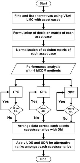
Figure 3.
Flow chart of proposed integrated decision-making planning (IDMP) approach.
In the proposed IDMP approach, initially in stage 1, two different VSAIs (VSAI_A and VSAI_B) with respective LMC aims at optimal sitting and sizing of assets in terms of finding suitable alternatives, as per Equations (1)–(11), respectively. The assumptions for both VSAI_A and VSAI_B are the same and can be found for normal load only in [30,31]. Later in stage 2, four different MCDM approaches are individually applied on the attainment of best alternative amongst technical criteria only, cost-economic criteria only, and overall (techno-economic) criteria across various cases of asset optimization, as per Equations (12)–(24).
In Figure 3, it is shown that the performance is assessed on the basis of technical performance evaluation (TPE), cost-economic performance evaluation (CPE), and overall combined (techno-economic) performance evaluation (OPE). Finally, in stage 3, UDM is applied and the best solution amongst multiple MCDM is sorted out on the basis of their respective UDM scores (UDS) of each case as per Section 2.4, particularly Equation (25). The achieved UDS will define new UDR of alternatives across multiple MCDM methodologies. The weights throughout each MCDM methods have been considered as equal or unbiased weighting since such weight is mostly utilized in most of the planning problems involving conflicting criteria. All the predetermined alternatives and the trade-off final solution achieved are subjected to practical system constraints.
3.2. Computation Procedure of Proposed IDMP Approach for Alternatives Selection and Case Studies
The overall computation method for VSAI_A and VSAI_B reported in [30,31] is essentially the same with a little difference. The LMC approach integrated with each VSAI is the same. The decision variables (DV) for optimal asset placement are based on type, size, and the number of assets. In [30], two variants of the planning approach were based on VSAI_A and LMC, whereas in [31], a single approach was presented based on VSAI_B and LMC. The assets are considered on the basis of numbers achieved in the previous publications [30,31]. The alternatives with DG were evaluated across normal load levels in [30], whereas the alternatives with DG only and asset sets (REG + D-STATCOM) were evaluated across normal load levels [31]. However, the abovementioned assets (DG only and REG + D-STATCOM) were evaluated across load growth levels for this study. The alternatives were achieved as follows:
- Alternate 1 (A1): 1×DG [30] or 1×asset set (REG + D-STATCOM) with VSAI_A and LMC.
- Alternate 2 (A2): 1×DG or 1×asset set (REG + D-STATCOM) with VSAI_B and LMC [31].
- Alternate 3 (A3): 2×DG [30] or 2×asset sets (REG + D-STATCOM) with VSAI_A and LMC.
- Alternate 4 (A4): 2×DG or 2×asset sets (REG + D-STATCOM) with VSAI_B and LMC [31].
- Alternate 5 (A5): 3×DG [30] or 3×asset sets (REG + D-STATCOM) with VSAI_A and LMC.
- Alternate 6 (A6): 3×DG [30] or 3×asset sets (REG + D-STATCOM) with VSAI_A and LMC.
- Alternate 7 (A7): 3×DG or 3×asset sets (REG + D-STATCOM) with VSAI_B and LMC [31].
All of the above seven alternatives have been evaluated in four cases across four MCDM methodologies under normal load (NL), load growth (LG) across five years, and optimal load growth (OLG) across five years, respectively. In NL, the current load is considered, and all the cases are evaluated. In LG, a 7.5% increment in load per annum is considered across five years, and asset sizing obtained during NL is retained as constant. In OLG, optimal asset sizing is considered across incremented load across five years. The OLG corresponds to the reinforcement required to maintain a solution after a planning horizon is over. The cases for evaluation with respective scenarios are TPE across technical criteria, CPE across cost-related criteria, and OPE across combined techno-economic criteria, respectively. The nomenclature of considered cases with respective scenarios for overall evaluation in this paper is presented as follows.
- Case 1: DGs only assets placements in MDN operating at 0.90 lagging power factor (LPF).
- Case 2: DGs only assets placements in MDN operating at 0.85 LPF.
- Case 3: Asset set (REG + D-STATCOM) placements in MDN equal to 0.90 LPF.
- Case 4: Asset set (REG + D-STATCOM) placements in MDN equal to 0.85 LPF.
In all of the above-mentioned four cases with respective designations, each case (C#) has been evaluated across the following scenarios of MCDM evaluations under various load levels as presented below.
- Scenario 1 (NL):
- Case 1 (C1_NL): TPE, CPE and OPE with WSM under NL.
- Case 2 (C2_NL): TPE, CPE and OPE with WPM under NL.
- Case 3 (C3_NL): TPE, CPE and OPE with TOPSIS under NL.
- Case 4 (C4_NL): TPE, CPE and OPE with PROMETHEE under NL.
- Scenario 2 (LG):
- Case 1 (C1_LG): TPE, CPE and OPE with WSM under LG.
- Case 2 (C2_LG): TPE, CPE and OPE with WPM under LG.
- Case 3 (C3_LG): TPE, CPE and OPE with TOPSIS under LG.
- Case 4 (C4_LG): TPE, CPE and OPE with PROMETHEE under LG.
- Scenario 3 (OLG):
- Case 1 (C1_OLG): TPE, CPE and OPE with WSM under OLG.
- Case 2 (C2_OLG): TPE, CPE and OPE with WPM under OLG.
- Case 3 (C3_OLG): TPE, CPE, and OPE with TOPSIS under OLG.
- Case 4 (C4_OLG): TPE, CPE and OPE with PROMETHEE under OLG.
Later, UDM is applied across all cases under all the above-mentioned cases with respective scenarios for a unanimous solution via UDS and the result attained in terms of UDR. The highest UDS value refers to the best solution with the highest UDR.
3.3. Constraints Considered in Simulations
The following main constraints [30,31] have been considered in this study. It was ensured that the simulations do not result in a solution that results in reverse power flow towards substation. It is considered that active and reactive power contribution from substation (PSS, QSS) and DG or other asset units (PDG, QDG) must have a balance that is equal to active and reactive power load consumption (PLD, QLD) along with associated active and reactive power losses (PLoss, QLoss) in MDN.
(PSS + QSS) + (PDG + QDG) = (PLD + QLD) + (PLoss + QLoss)
The magnitude of the voltage at each node/bus “n” in MDN must not exceed the specified limit of 0.95 P.U to 1.05 P.U.
0.95 ≤ Vn ≤ 1.05; n = 1, 2, 3, 4 … m
The LPF of DG is kept within limits considering an allowable variation of ±3%.
3.4. Simulation Setup
The proposed IDMP approach is tested on the 33-bus test distribution network (TDN), as displayed in Figure 4. The PLD and QLD in the 33-bus TDN account for 3715 KW and 2300 KVAR, whereas PLoss and QLoss account for 210.9 KW and 143.02 KVAR during a base case under normal load, respectively. In the case of load growth, The P and Q loads are 5333.363 KW and 3301.95 KVAR, respectively. The P and Q losses during load growth account for 450.65 KW and 305.17 KVAR, respectively.
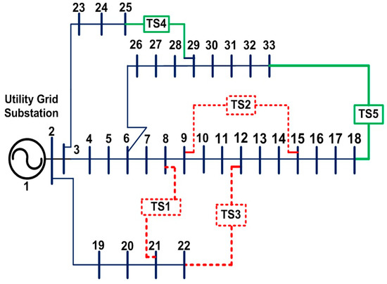
Figure 4.
33-bus (meshed configured) test distribution system.
The test MDN consists of four branches and five TSs. The 33-bus TDN is converted into a multiple-loop configured MDN by closing TS4 and TS5 (highlighted in green solid line) and results in two loop currents (ILp1 and ILp2) across two TB, respectively. The load or power flow analysis regarding the 33-bus TDN is obtained in terms of numerical values from equivalent models and has been implemented on MATLAB R2018a. The test setup is developed in SIMULINK and numerical values are called in m-files where the proposed approach is evaluated into achieved results. Initially, the assets are placed on designated locations given by VSAIs in [30,31]. The base case model is made in SIMULINK and values are called in m-file that indicate the weakest nodes as shown in [30,31]. Later, the numerical values were obtained from simulation setup in SIMULINK and are run until the condition where loop currents across TB are near zero and voltages across the respective nodes are equal with the optimal sizing of assets considering termination criteria of 1%. Finally, on termination, the achieved values are called in a program made of m-files (MATLAB 2018a), where the proposed IDMP approach is evaluated with various matrices and is represented in the following Section 3.5.
The proposed IDMP approach is evaluated across various load and generation levels in terms of snapshot analysis. Although the IDMP approach seems dynamic, the snapshot analysis considering NL, LG, and OLG is evaluated in terms of steady-state analysis. The approach simplifies the requirement of dynamic analysis and gives a big picture in terms of steady-state analysis.
The asset sitting and sizing cases are evaluated across NL, where optimal sizing of assets is achieved in terms of performance evaluations. In LG, the generation from NL cases is kept constant and an increase in load after five years is considered for evaluation of the assets performance across the planning horizon. In OLG, the assets reinforcements required for optimal performance after planning horizon are evaluated.
3.5. Performance Evaluation Indicators (PEI)
The technical and cost-economic indices for performance evaluation are illustrated in Table 3 and Table 4 and all relations have been taken from our previous publications in [30,31].
Table 3.
Technical indices for performance evaluation (designated as technical performance evaluation (TPE)).
Table 4.
Cost-economic indices for performance evaluation (designated as cost-economic performance evaluation (CPE)).
4. Results and Discussions
The IDMP approach is applied in three stages as aforementioned in Section 3.1 and Section 3.2. The first stage is employed for the layout (sitting and sizing) of numerous assets such as DG and D-STATCOM units in the MDN. The proposed integrated approach consists of two parts; VSAIs [30,31] are applied for potential assets (DG and REG + DSTATCOM) locations for sitting and LMC for optimal asset sizing.
In total, seven alternatives were shortlisted encapsulating four cases of assets sitting and sizing, across NL, LG, and OLG, respectively. Case 1 covers DGs operating at 0.90 LPF, case 2 covers DG operating at 0.85 LPF, and case 3 covers renewable DG such as PV system that contributes active power (P) only and reactive component (Q) comes from D-STATCOM. The contribution from the set of these two assets i.e., the P and Q contributions, is equal to 0.90 PF. In case 4, P and Q contributions are equal to that of one DG contributing at 0.85 LPF. Cases 1–2 are different than cases 3–4 in such a manner that DG only cases can be subjected to reactive power instability whereas in later cases, the power sources are decoupled. So, a comparative analysis is justified in terms of performance analysis.
In the second stage, four MCDM methodologies are applied to find out the best solution amongst the sorted alternatives. In the third stage, unanimous decision making (UDM) is applied to find out a common best solution in the achieved solutions that may vary on the basis of MCDM techniques.
The proposed IDMP approach is evaluated across technical, cost-economic, and combined techno-economic criteria of conflicting nature. Since the cost-related criteria may differ from various asset types, for the sake of composite evaluation, separated P and Q injections are considered.
4.1. Case 1 under Normal Load (C1_NL): DGs Only Placements in MDN Operating at 0.90 LPF
4.1.1. Initial Evaluation of Alternatives in Case 1 under Normal Load (C1_NL)
The initial evaluation of C1_NL for each alternative is shown in terms of TPE and CPE are shown in Table 5. The numerical values refer to evaluated indices values as potential criteria results obtained for seven alternatives referring to DG only asset placement operating at 0.90 LPF under NL. The reason being such a PF is favored by utilities.
Table 5.
Techno-economic evaluation analysis in case 1 (C1_NL) for 33-bus MDN.
The four considered MCDM techniques have evaluated across each alternative in TPE and CPE separately. In the case of OPE, all criteria except substation capacity are utilized in further evaluation with MCDM techniques. It is worth mentioning that in the all calculations of CPE and OPE cases, values of AIC were considered as achieved in [31].
4.1.2. MCDM Evaluation of Alternatives in Case 1 Under Normal Load (C1_NL)
The MCDM evaluations for C1_NL are illustrated in Figure 5a–d. The detailed numerical evaluations can be found in the supplementary file. Here, only the preference scores were illustrated in the figures to sort out a best alternative on the basis of TPE, CPE, and OPE evaluation per MCDM technique against each respective scenario. Refer to Table 5 for respective TPE and CPE in terms of numerical details without normalization. The rank of the alternatives in C1_NL are shown in Table 6.
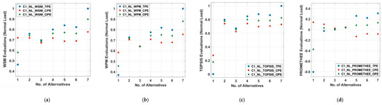
Figure 5.
MCDM evaluations for C1_NL in 33-bus MDN: (a) weighted sum method (WSM) scores; (b) weighted product method (WPM) scores; (c) technique for order preference by similarity to ideal solution (TOPSIS) scores; (d) preference ranking organization method for enrichment of evaluations (PROMETHEE) scores.
Table 6.
Order of the ranks across TPE, CPE, and OPE in C1_NL for 33-bus MDN.
As per the results, initially, the best alternative in TPE and OPE based evaluations is A7 as highlighted in Table 6, whereas in CPE there is no unanimous optimal solution. It is also observed that change of rank is more visible in CPE based evaluations with every MCDM approach.
After applying UDM with respective score and resulting alternative rank, the unanimous best solution utilizing various MCDM methodologies across TPE, CPE, and OPE are A7 (UDS=28 and UDR=1), A4 (UDS=22 and UDR=1), and A7 (UDS=28 and UDR=1); respectively. The UDM with UDS and UDR across TPE, CPE and OPE in C1_NL have highlighted in bold text as shown in Table 6.
4.2. Case 2 Under Normal Load (C2_NL): DGs Only Assets Placements in MDN Operating at 0.85 LPF
4.2.1. Initial Evaluation of Alternatives in Case 2 Under Normal Load (C2_NL)
The initial evaluation of case 2 (C2_NL) for each alternative is shown in terms of TPE and CPE is shown in Table 6. The numerical results were evaluated for seven alternatives using DG only asset placement operating at 0.85 LPF under NL.
The MCDM techniques were evaluated across each alternative in TPE and CPE in the same manner as in C1. The main reason for considering the 0.85 LPF of DG is close to that of DN is that it provides more reactive power support at load centers compared to those DGs operating at 0.90 LPF. It is advocated in various publications that such an arrangement results in achieving a better system LM with considerably better VP.
4.2.2. MCDM Evaluation of Alternatives in Case 2 under Normal Load (C2_NL)
The MCDM evaluations for case 2 (C2_NL) are illustrated in Figure 6a–d. The evaluation in terms of best and worst alternative with respective scores are shown below.
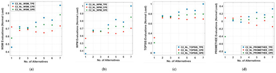
Figure 6.
MCDM evaluations for C2_NL in 33-bus MDN: (a) WSM scores; (b) WPM scores; (c) TOPSIS scores; (d) PROMETHEE scores.
Refer to Table 7 for respective TPE and CPE in terms of numerical details without normalization. The rank of the alternatives in C2_NL is shown in Table 8. As per MCDM results, the best alternative in TPE is A7, whereas no unanimous solution is obtained in CPE and OPE. However, they are dominated by A7. After applying UDM with the best solution in TPE, CPE, and OPE are A7 (UDS=28 and UDR=1), A3 (UDS=23 and UDR=1), and A7 (UDS=27 and UDR=1); respectively. The UDM with UDS and UDR across TPE, CPE and OPE in C2_NL have highlighted in bold text as shown in Table 8.
Table 7.
Techno-economic evaluation analysis in case 2 (C2_NL) for 33-bus MDN.
Table 8.
Order of the ranks across TPE, CPE, and OPE in C2_NL for 33-bus MDN.
4.3. Case 3 Under Normal Load (C3_NL): Asset Set (REG + D-STATCOM) Placements Equivalent to 0.90 LPF
4.3.1. Initial Evaluation of Alternatives in Case 3 under Normal Load (C3_NL)
The initial evaluation of case 3 (C3_NL) for each alternative in terms of TPE and CPE is shown in Table 9. The numerical values refer to evaluated indices values for seven alternatives utilizing an asset set of REG (i.e., PV) and D-STATCOM for providing active and reactive power source, which is equal to single DG operating at 0.90 LPF under NL. The MCDM techniques were evaluated across each alternative is in the same manner as previous cases.
Table 9.
Techno-economic evaluation analysis in case 3 (C3_NL) for 33-bus MDN.
4.3.2. MCDM Evaluation of Alternatives in Case 3 Under Normal Load (C3_NL)
The MCDM evaluations for case 3 (C3_NL) are illustrated in Figure 7a–d. Refer to Table 9 for respective TPE and CPE in terms of numerical details without normalization. The rank of the alternatives in C3_NL is shown in Table 10.
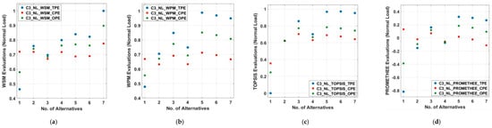
Figure 7.
MCDM evaluations for C3_NL in 33-bus MDN: (a) WSM scores; (b) WPM scores; (c) TOPSIS scores; (d) PROMETHEE scores.
Table 10.
Order of the ranks across TPE, CPE, and OPE in C3_NL for 33-bus MDN.
As per the results, the best alternative is A5 in OPE only. After applying UDM, the best solutions in TPE, CPE, and OPE were A5 (UDS=28 and UDR=1), A3 (UDS=23 and UDR=1), and A5 (UDS=26 and UDR=1); respectively. The UDM with UDS and UDR across TPE, CPE and OPE in C3_NL have highlighted in bold text as shown in Table 10.
4.4. Case 4 Under Normal Load (C4_NL): Asset Set (REG + D-STATCOM) Placements Equivalent to 0.85 LPF
4.4.1. Initial Evaluation of Alternatives in Case 4 under Normal Load (C4_NL)
The initial evaluation of case 4 (C4_NL) for each alternative is shown in terms of TPE and CPE is shown in Table 11. The numerical values were evaluated for seven alternatives utilizing an asset set of renewable DG i.e., PV and D-STATCOM for providing active and reactive power source, which is equal to single DG operating at 0.85 LPF under NL.
Table 11.
Techno-economic evaluation analysis in case 4 (C4_NL) for 33-bus MDN.
The MCDM techniques were evaluated across each alternative in the same manner as previous cases as illustrated in Figure 8a–d.
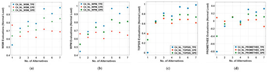
Figure 8.
MCDM evaluations for C4_NL in 33-bus MDN: (a) WSM scores; (b) WPM scores; (c) TOPSIS scores; (d) PROMETHEE scores.
4.4.2. MCDM Evaluation of Alternatives in Case 4 Under Normal Load (C4_NL)
The MCDM evaluations for case 4 are illustrated in Figure 8a–d. Refer to Table 11 for respective TPE and CPE in terms of numerical details without normalization.
The rank of the alternatives in C4_NL is shown in Table 12. As per the results, the best alternative is A7 in TPE and A5 in OPE. After applying UDM, the best solutions in TPE, CPE, and OPE were A7 (UDS=28 and UDR=1), A3 (UDS=24 and UDR=1), and A5 (UDS=28 and UDR=1); respectively. The UDM with UDS and UDR across TPE, CPE and OPE in C4_NL have highlighted in bold text as shown in Table 12.
Table 12.
Order of the ranks across TPE, CPE, and OPE in C4_NL for 33-bus MDN.
4.5. Case 1 Under Load Growth (C1_LG): DGs Only Assets Placements in MDN Operating at 0.90 LPF
4.5.1. Initial Evaluation of Alternatives in Case 1 Under Load Growth (C1_LG)
The initial evaluation from the perspective of TPE and CPE, of C1_LG, is shown in Table 13. The case of load growth refers to the condition, in which asset sitting and sizing achieved during normal load is kept constant across a planning horizon and load is incremented annually at a rate of 7.5%. The main aim of this evaluation is to find the change in the rank of alternatives initially evaluated as optimal ones.
Table 13.
Techno-economic evaluation analysis in case 1 (C1_LG) for 33-bus MDN.
The MCDM evaluation under LG shows a dip in achieved preference score, as well as a change in the ranks of the alternatives. This analysis indicates the change of rank and respective impacts on the active MDN across the LG. Also, the initially optimal solution may not remain feasible and the sub-optimal one may become a better choice, after a certain planning horizon.
4.5.2. MCDM Evaluation of Alternatives in Case 1 under Load Growth (C1_LG)
The MCDM evaluations for case 1 are illustrated in Figure 9a–d. The rank of the alternatives in C1_LG is shown in Table 14. As per the results, the best alternative in TPE is A6, whereas there is not a unanimous solution in CPE and OPE, respectively. After applying UDM, the best solutions in TPE, CPE, and OPE are A6 (UDS=28 and UDR=1), A3 (UDS=23 and UDR=1), and A6 (UDS=26 and UDR=1); respectively. The UDM with UDS and UDR across TPE, CPE and OPE in C1_LG have highlighted in bold text as shown in Table 14.
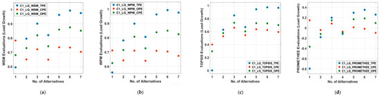
Figure 9.
MCDM evaluations for C1_LG in 33-bus MDN: (a) WSM scores; (b) WPM scores; (c) TOPSIS scores; (d) PROMETHEE scores.
Table 14.
Order of the ranks across TPE, CPE, and OPE in C1_LG for 33-bus MDN.
4.6. Case 2 under Load Growth (C2_LG): DGs Only Assets Placements in MDN Operating at 0.85 LPF
4.6.1. Initial Evaluation of Alternatives in Case 2 under Load Growth (C2_LG)
The initial evaluation of case 2 (C2_LG) for each alternative under load growth in terms of TPE and CPE is shown in Table 15.
Table 15.
Techno-economic evaluation analysis in case 2 (C2_LG) for 33-bus MDN.
4.6.2. MCDM Evaluation of Alternatives in Case 2 under Load Growth (C2_LG)
The MCDM evaluations for case 2 (C2) under load growth are illustrated in Figure 10a–d. The rank of the alternatives in C2 under LG (C2_LG) is shown in Table 16. As per the results, the best alternative in TPE is A7, whereas no unanimous solution is obtained in CPE and OPE. After applying UDM, the best solutions in TPE, CPE, and OPE are A7 (UDS=28 and UDR=1), A3 (UDS=24 and UDR=1), and A5 (UDS=25 and UDR=1); respectively. The UDM with UDS and UDR across TPE, CPE and OPE in C2_LG have highlighted in bold text as shown in Table 16.
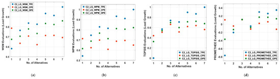
Figure 10.
MCDM evaluations for C2_LG in 33-bus MDN: (a) WSM scores; (b) WPM scores; (c) TOPSIS scores; (d) PROMETHEE scores.
Table 16.
Order of the ranks across TPE, CPE, and OPE in C2_LG for 33-bus MDN.
4.7. Case 3 Under Load Growth: Asset Set (REG + D-STATCOM) Placements Equivalent to 0.90 LPF (C3_LG)
4.7.1. Initial Evaluation of Alternatives in Case 3 under Normal Load (C3_LG)
The initial evaluation of C3_LG for each alternative in terms of TPE and CPE is shown in Table 11.
4.7.2. MCDM Evaluation of Alternatives in Case 3 under Load Growth (C3_LG)
The MCDM evaluations for C3_LG are illustrated in Figure 11a–d. Refer to Table 17 for respective TPE and CPE in terms of numerical details without normalization. The rank of the alternatives in C3 under LG is shown in Table 18. As per the results, the best alternative in TPE is A6, whereas there are no unanimous solutions in CPE and OPE, respectively. After applying UDM, the best solutions in TPE, CPE, and OPE are A6 (UDS=28 and UDR=1), A3 (UDS=23 and UDR=1), and A6 (UDS=26 and UDR=1), respectively. The UDM with UDS and UDR across TPE, CPE and OPE in C3_LG have highlighted in bold text as shown in Table 18.
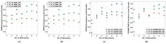
Figure 11.
MCDM evaluations for C3_LG in 33-bus MDN: (a) WSM scores; (b) WPM scores; (c) TOPSIS scores; (d) PROMETHEE scores.
Table 17.
Techno-economic evaluation analysis in case 3 (C3_LG) for 33-bus MDN.
Table 18.
Order of the ranks across TPE, CPE, and OPE in C3_LG for 33-bus MDN.
4.8. Case 4 Under Load Growth: Assets (DG + D-STATCOM) Placements Equivalent to 0.85 LPF (C4_LG)
4.8.1. Initial Evaluation of Alternatives in Case 4 Under Load Growth (C4_LG)
The initial evaluation of case 4 (C4_LG) for each alternative under LG in terms of TPE and CPE is shown in Table 19.
Table 19.
Techno-economic evaluation analysis in case 4 (C4_LG) for 33-bus MDN.
4.8.2. MCDM evaluation of alternatives in Case 4 under load growth (C4_LG)
The MCDM evaluations for C4_LG are illustrated in Figure 12a–d. The rank of the alternatives in C4_LG is shown in Table 20.
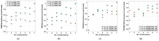
Figure 12.
MCDM evaluations for C4_LG in 33-bus MDN: (a) WSM scores; (b) WPM scores; (c) TOPSIS scores; (d) PROMETHEE scores.
Table 20.
Order of the ranks across TPE, CPE, and OPE in C4_LG for 33-bus MDN.
As per the results in Figure 12a–d and Table 20, the best alternative in TPE is A7, whereas there are no unanimous solutions in CPE and in OPE. After applying UDM, the best solutions in TPE, CPE, and OPE are A7 (UDS=28 and UDR=1), A3 (UDS=26 and UDR=1), and A5 (UDS=26 and UDR=1), respectively. The UDM with UDS and UDR across TPE, CPE and OPE in C4_LG have highlighted in bold text as shown in Table 20.
4.9. Case 1 Under Optimal Load Growth: DGs Only Assets Placements Operating at 0.90 LPF (C1_OLG)
4.9.1. Initial Evaluation of Alternatives in Case 1 Under Optimal Load Growth (C1_OLG)
The initial evaluation of C1_OLG is shown in Table 21, from the perspective of TPE and CPE.
Table 21.
Techno-economic evaluation analysis in case 1 (C1_OLG) for 33-bus MDN.
4.9.2. MCDM Evaluation of Alternatives in Case 1 Under Optimal Load Growth (C1_OLG)
The MCDM evaluations for case 1 are illustrated in Figure 13a–d. The rank of the alternatives in C1_OLG is shown in Table 22. As per the results, the best alternative in OPE is A5, whereas there is not a unanimous solution in TPE and CPE, respectively. After applying UDM, the best solutions in TPE, CPE, and OPE are A5 (UDS=24 and UDR=1), A3 (UDS=23 and UDR=1), and A5 (UDS=26 and UDR=1); respectively. The UDM with UDS and UDR across TPE, CPE and OPE in C1_OLG have highlighted in bold text as shown in Table 22.
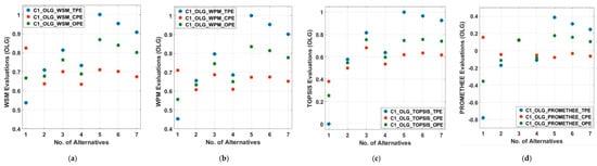
Figure 13.
MCDM evaluations for C1_OLG in 33-bus MDN: (a) WSM scores; (b) WPM scores; (c) TOPSIS scores; (d) PROMETHEE scores.
Table 22.
Order of the ranks across TPE, CPE, and OPE in C1_OLG for 33-bus MDN.
4.10. Case 2 under Optimal Load Growth: Dgs Only Assets Placements Operating at 0.85 LPF (C2_OLG)
4.10.1. Initial Evaluation of Alternatives in Case 2 under Optimal Load Growth (C2_OLG)
The initial evaluation of case 2 (C2_OLG) under OLG for each alternative in terms of TPE and CPE is shown in Table 23.
Table 23.
Techno-economic evaluation analysis in case 2 (C2_OLG) for 33-bus MDN.
4.10.2. MCDM Evaluation of Alternatives in Case 2 under Optimal Load Growth (C2_OLG)
The MCDM evaluations for case 2 (C2_OLG) under optimal load growth are illustrated in Figure 14a–d. The rank of the alternatives in C2_OLG is shown in Table 24. As per the results, the best alternative in OPE is A5, whereas no unanimous solution is obtained in CPE and OPE. After applying UDM, the best solutions in TPE, CPE, and OPE are A5 (UDS=26 and UDR=1), A5 (UDS=23 and UDR=1), and A5 (UDS=28 and UDR=1), respectively.
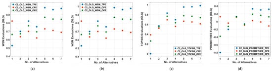
Figure 14.
MCDM evaluations for C2_OLG in 33-bus MDN: (a) WSM scores; (b) WPM scores; (c) TOPSIS scores; (d) PROMETHEE scores.
Table 24.
Order of the ranks across TPE, CPE, and OPE in C2_OLG for 33-bus MDN.
It can be seen in Table 24 from CPE (C2_OLG) that the UDS score of A1 and A3 is the same (UDS=22). As per the aforementioned rules devised for UDM in Section 2.5, the solution with the highest number of highest priority ranks will be given preference. Hence, alternative A1 (UDR=2) is given preference over A3 (UDR=3) for the second-best alternative despite having the same score from the viewpoint of UDS. The UDM with UDS and UDR across TPE, CPE and OPE in C2_OLG have highlighted in bold text as shown in Table 24.
4.11. Case 3 under Optimal Load Growth: Assets (REG + D-STATCOM) Placements Equal to 0.90 LPF (C3_OLG)
4.11.1. Initial Evaluation of Alternatives in Case 3 under Optimal Normal Load (C3_OLG)
The initial evaluation of C3_OLG for each alternative in terms of TPE and CPE under OLG is shown in Table 25.
Table 25.
Techno-economic evaluation analysis in case 3 (C3_OLG) for 33-bus MDN.
4.11.2. MCDM Evaluation of Alternatives in Case 3 Under Optimal Load Growth (C3_OLG)
The MCDM evaluations for C3_OLG are illustrated in Figure 15a–d. Refer to Table 25 for respective TPE and CPE in terms of numerical details without normalization. The rank of the alternatives in C3_OLG is shown in Table 26. As per the results, the best alternative in TPE is A5, whereas there are no unanimous solutions in CPE and OPE. After applying UDM, the best solutions in TPE, CPE, and OPE are A5 (UDS=28 and UDR=1), A3 (UDS=23 and UDR=1), and A5 (UDS=26 and UDR=1); respectively. The UDM with UDS and UDR across TPE, CPE and OPE in C3_OLG have highlighted in bold text as shown in Table 26.
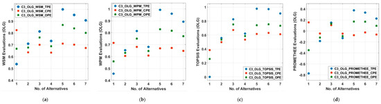
Figure 15.
MCDM evaluations for C3_OLG in 33-bus MDN: (a) WSM scores; (b) WPM scores; (c) TOPSIS scores; (d) PROMETHEE scores.
Table 26.
Order of the ranks across TPE, CPE, and OPE in C3_OLG for 33-bus MDN.
4.12. Case 4 Under Optimal Load Growth: Asset REG + D-STATCOM Placements Equal to 0.85 LPF (C4_OLG)
4.12.1. Initial Evaluation of Alternatives in Case 4 under Optimal Load Growth (C4_OLG)
The initial evaluation of case 4 (C4_OLG) for each alternative under LG in terms of TPE and CPE is shown in Table 27.
Table 27.
Techno-economic evaluation analysis in case 4 (C4_OLG) for 33-bus MDN.
4.12.2. MCDM Evaluation of Alternatives in Case 4 under Optimal Load growth (C4_OLG)
The MCDM Evaluations for Case 4 (C4_OLG) under OLG Are Illustrated in Figure 16a–d. The rank of the alternatives in C4_OLG is shown in Table 28. As per the results, the best alternative in TPE and CPE is A5, whereas there are no unanimous solutions in CPE. After applying UDM, the best solutions in TPE, CPE, and OPE are A5 (UDS=28 and UDR=1), A5 (UDS=23 and UDR=1), and A5 (UDS=28 and UDR=1); respectively. The UDM with UDS and UDR across TPE, CPE and OPE in C4_OLG have highlighted in bold text as shown in Table 28.
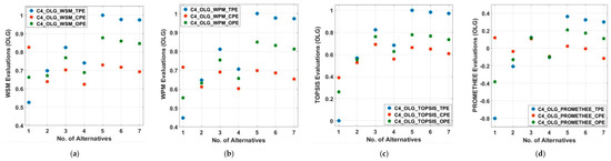
Figure 16.
MCDM evaluations for C4_OLG in 33-bus MDN: (a) WSM scores; (b) WPM scores; (c) TOPSIS scores; (d) PROMETHEE scores.
Table 28.
Order of the ranks across TPE, CPE, and OPE in C4_OLG for 33-bus MDN.
In all the cases of the proposed IDMP approach above, it is found that the TPE of each respective case has less variance compared to other cases. The OPE shows the maximum variance while the CPE shows the maximum variance when evaluated across various MCDM methodologies.
5. Comparison and Validation Analysis
The proposed IDMP approach aimed at (multiple-loop configured) MDN is evaluated on 33-bus TDN and validated via comparative analysis of achieved results with the findings in the available literature, respectively. The comparison section consists of two sub-sections. In the first section, achieved results are compared with each other along with the change of rank in different cases of asset sitting and sizing. In the following case, the achieved results are compared with the results reported in the reviewed literature.
5.1. Results Comparison with Achieved Results
The achieved results for self-comparison are presented in Table 29. In Table 29, an overview of performance evaluation in the proposed IDMP approach across technical, cost, and overall (techno-economic) criteria were evaluated under various load and generation conditions in 33-bus TDS.
Table 29.
Overview performance evaluation analysis for all evaluated cases of IDMP across various evaluations for self-comparison of change in ranks.
In case 1 (C1), from the perspective of technical evaluation, the TPE across NL, LG, and OLG as designated by TPE_NL, TPE_LG, and TPE_OLG are presented after applying UDM. The relative comparison from the viewpoint of rank changed (RC) designated by RC1, between respective cases of NL and LG, reveals that in C1, all ranks are changed under TPE except A7. The RC2 among NL and OLG reveals the same. However, in RC3, the only ranks changed amongst solutions are A1–A3.
In C1, from the perspective of cost-economic evaluation, the CPE across NL, LG, and OLG as designated by CPE_NL, CPE_LG, and CPE_OLG are presented after applying UDM. The results indicate that in RC1 and RC2, all the ranks of possible solutions (alternatives) have changed. However, in RC3, the ranks changed in the achieved solutions are A1–A4, respectively.
In C1, from the perspective of overall (techno-economic) performance evaluation, the OPE across NL, LG, and OLG as designated by OPE_NL, OPE_LG, and OPE_OLG are presented after applying UDM. The achieved results indicate that in RC1 and RC2, all the ranks of alternatives have changed except A7. However, in RC3, the ranks changed in the achieved solutions are A1–A2.
In C2, in terms of TPE, RC1 shows the rank change in A5, A6, and A7. In RC2, the change of ranks is found in A1–A2, A4–A6. In RC3, the change of rank is found in A1 and A2. In terms of CPE, in RC1, change of ranks is observed in A1–A2. In RC2, ranks change is observed in all alternatives. In RC3, change of rank is observed in A1–A2 and A4. From the viewpoint of OPE, in RC1, change of rank is observed in all alternatives except A7. In RC2, rank change is observed in all except A2 and A7. In RC3, rank change is observed in solutions designated by A2–A4.
It is also observed that in C1–C2, DG can be subjected to reactive power support limit whereas in C3–C4, when REG and D-STATCOM are decoupled, overall better performance is achieved as mentioned throughout the paper, as demonstrated in the results and discussion section.
In C3, in terms of TPE, RC1 shows the rank change in A1–A3. In RC2, no change of ranks is found. In RC3, the change of rank is found in A1–A3. In terms of CPE, in RC1, change of ranks is observed in A1–A4. In RC2, ranks change is observed in all alternatives except A3 and A5. In RC3, change of rank is observed in A3–A4 and A6–A7. From the viewpoint of OPE, in RC1, change of rank is observed in all alternatives except A1–A2. In RC2, in respective comparison, all ranks changed. In RC3, rank change is observed in solutions designated by A1–A2.
In C4, in terms of TPE, RC1 shows no change of rank amongst stated alternatives. In RC2, change of ranks is found in A1–A3. In RC3, the change of rank is found in A1–A3. In terms of CPE, in RC1, change of ranks is observed in A2–A4. In RC2, ranks change is observed in alternatives A1–A4. In RC3, change of rank is observed in A1–A3. From the viewpoint of OPE, in RC1, change of rank is observed in A2–A3. In RC2, in respective comparison, no ranks have changed. In RC3, rank change is observed in solutions designated by A2–A3.
5.2. Results Comparison with Reported Results
The proposed IDMP approach aims at MDN is evaluated on the 33-bus TDS and validated via comparative analysis of achieved results with the findings in the available literature, respectively. The achieved results are compared on the basis of best-achieved solutions obtained in each case (C1–C4) via proposed approach across NL, LG, and OLG via each TPE, CPE, and OPE, respectively.
5.2.1. Evaluated Results Comparison of C1_NL for DGs Operating at 0.90 LPF
The evaluation comparison of case 1 (C1_NL) for each alternative in terms of TPE, CPE, and OPE are shown in Table 30. The achieved results are compared with multi-objective hybrid GA and TOPSIS approach in [42] and the multi-objective centric hybrid sensitivity-based approach in [53]. It is observed that the proposed alternative A7 in IDMP during C1_NL is best from the viewpoint of TPE and OPE, whereas A4 outperforms on the basis of CPE. Note that the achieved results that outperformed the compared works are shown in bold text, throughout this section.
Table 30.
Comparisons of results with C1_NL for 33-bus TDN (DG@LPF = 0.90).
5.2.2. Evaluated Results Comparison of C2_NL for DGs Operating at 0.85 LPF
The evaluation comparison of case 2 (C2_NL) for each alternative under NL is shown in terms of TPE, CPE, and OPE are shown in Table 31. The best-achieved alternatives are compared with the multi-objective hybrid GA and TOPSIS approach in [42], loss sensitivity factor (LSF) and simulated annealing (SA)-based hybrid method in [54], heuristic-based krill herd algorithm in [55], and ant colony optimization (ACO) and artificial bee colony (ABC) as reported in [56], respectively. It is worth mentioning that the reported studies are more focused on technical evaluation, and comparison with CPE in the reported work is only presented for reference. It is observed that the proposed alternative A7 in IDMP during C2_NL is best from the viewpoint of TPE and OPE, whereas A3 outperforms on the basis of CPE. The outperformed results have shown in bold text for comparative analysis.
Table 31.
Comparisons of results with C2_NL for 33-bus TDN (DG@LPF = 0.85).
5.2.3. Evaluated Results Comparison of C3_NL and C4_NL for REG + D-STATCOM
The evaluation comparison of C3_NL and C4_NL for each alternative in terms of TPE, CPE, and OPE are shown in Table 32 and Table 33 respectively.
Table 32.
Comparisons of results with C3_NL for 33-bus TDN (REG + D-STATCOM@LPF = 0.9).
Table 33.
Comparisons of results with C4_NL for 33-bus TDN (REG + D-STATCOM@LPF = 0.85).
The best-achieved alternatives in C3_NL are compared in Table 18 with well-established approaches such as the best-achieved alternatives and compared with well-established methods such as hybrid fuzzy ant colony optimization approach in [34], multiple attribute decision-making (MCDM) methods such as TOPSIS and PROMETHEE in [35], and sensitivity-based approach in [57]. It is found that A3 in [30] amongst other alternatives in the C3_NL of the proposed IDMP method provides a big picture on the basis of CPE. Moreover, on the basis of TPE and OPE, the findings of the A7 solution are in close agreement with the reported works, hence validating the proposed approach under NL.
The findings of C4_NL are compared in Table 18 with reported works such as hybrid fuzzy ant colony optimization method in [34] and cuckoo search algorithm (CSA) in [37]. The reported work is in close agreement with solution A7 in [37] on the basis of TPE, A3 [30] and A5 [30] on the basis of CPE and OPE, which indicates the validity of proposed approach with assets such as REG and DSTATCOM, respectively.
5.2.4. Evaluated Results Comparison of C1_LG-C4_LG
The evaluation comparison of all four cases under load growth is compared with the results of the sensitivity-based approach reported in [57]. The results are compared for the cases C1_LG and C2_LG in Table 34 for the assets considering DG only case operating at 0.90 LPF and 0.85 LPF, respectively. The assets in both cases, such as DGs only, are capable of contributing both active and reactive power. The case for LG is presented for the reason that the LG impact from the perspective of assets considered has to be evaluated and relative impacts from the techno-economic perspective must be assessed. From the viewpoint of C1_LG, it is found that solution A3 via CPE and A6 via TPE and OPE is the best that even outperforms the results in [57]. From the standpoint of C2_LG, A7 (in TPE), A3 (in CPE), and A5 in OPE outperform the results stated in [57].
Table 34.
Comparisons of results with C1_LG and C2_LG for 33-bus TDN (DG@LPF = 0.90, 0.85).
The results are compared for the cases C3_LG and C4_LG in Table 35 for the assets such as REG and D-STATCOM, which are decoupled in comparison with DG only cases reported in C1_LG and C2_LG. However, they contribute active and reactive power that is equal to one DG supplying P and Q either at 0.90 or 0.85 LPF. The P contributes via REG and Q support is provided by D-STATCOM. It is found that the achieved results outperform reported works on the basis of TPE, CPE, and OPE.
Table 35.
Comparisons of results with C3_LG and C4_LG for 33-bus TDN (REG + D-STATCOM).
5.2.5. Evaluated Results Comparison of C1_OLG-C4_OLG
The evaluation comparison of achieved results in C1_OLG and C2_OLG are shown in Table 36, the multi-aspect results outperform the reported results in [57].
Table 36.
Comparisons of results with C1-C2 under OLG for 33-bus TDS (DG@LPF = 0.90, 0.85).
The evaluation results of C3_OLG and C4_OLG are compared in Table 37 with hybrid particle swarm optimization (PSO) and GAMS in [36], and sensitivity-based approach in [57]. The results from the proposed work outperforms the reported works from the perspective of better performance and optimal sizing assets, as shown in bold text shown throughout this section.
Table 37.
Comparisons of results with C4-C4 under OLG for 33-bus TDS (REG + D-STATCOM).
6. Conclusions
The active meshed distribution network is considered as a model of future smart distribution networks, which are anticipated to exhibit better performance and reliability through interconnection. Practical planning problems must be capable of encapsulating solutions that must satisfy conflicting criteria across the planning horizon. Thus, this works offers an IDMP approach aimed at various types of asset sitting and sizing across the normal load and load growth levels in a meshed distribution network. The assets considered in this study are synchronous generators operating at various lagging power factors (LPF) and capable of giving active and reactive powers and renewable DGs like photovoltaic (PV) system (contributes active power only) and D-STATCOM (contributes reactive power only). The methodology consists of an initial evaluation of alternatives with the voltage stability assessment indices-loss minimization condition (VSAI-LMC)-based method with single and multiple assets. Later, four MCDM methodologies are applied to sort out the best solution amongst the achieved alternatives. Finally, unanimous decision-making (UDM) is applied to find out one trade-off solution amongst achieved ranks of various MCDM methods. The methodology is applied across technical only (TPE), cost-economic only (CPE), and overall techno-economic (OPE) performance evaluations across four cases of assets sitting and sizing. All four cases are evaluated across the normal load, load growth, and optimal load growth. The detailed performance analysis is applied across the meshed configured 33-bus test distribution network. The achieved results across all cases after comparison with the credible results reported in the literature have both outperformed and displayed close agreement, resulting in the validation of the proposed IDMP approach. The proposed approach with techno-economic performance evaluation among conflicting criteria across the time scale reduces the need for sensitivity analysis and provides a range of trade-off solutions across various performance metrics. The overall approach in this paper aims to offer decision-makers a wide variety of optimal solutions among conflicting criteria considering various cases of asset optimization.
Supplementary Materials
The following are available online at https://www.mdpi.com/1996-1073/13/6/1444/s1.
Author Contributions
S.A.A.K. (First and corresponding author), U.A.K. (Second author), H.W.A. (Third Author), S.A. (Fourth Author) and D.R.S. (Fifth author) offers the presented study. The roles are defined as per the order of authors. S.A.A.K. is responsible for conceptualization, methodology, formal analysis, and investigation, resources, writing (original draft preparation), writing (review and editing), supervision, project administration, funding acquisition. U.A.K., H.W.A., and S.A. are responsible for formal analysis, investigation, software, validation, visualization, and writing (original draft preparation). D.R.S. is responsible for supervision and review. All authors have read and agreed to the published version of the manuscript
Funding
This research received no external funding. This research was supported and conducted in the United States-Pakistan Center of Advanced Studies in Energy (USPCAS-E), National University of Science and Technology (NUST), Islamabad, Pakistan. The APC is funded internally by National University of Science and Technology (NUST), Islamabad, Pakistan.
Conflicts of Interest
The authors declare no conflict of interest.
Abbreviations
The following abbreviations have used in this paper.
| ACD | Annual cost of D-STATCOM |
| ADN | Active distribution Network |
| AIC | Annual investment cost |
| AFc | Annualized factor (of cost) in USD $ |
| C (#) | Case (No. = 1, 2, 3, 4) |
| Ct | Annual cost based on interest-rate |
| CPDG | Cost of active power from DG |
| CPE | Cost-economic performance evaluation |
| CQDG | Cost of reactive power from DG |
| CUc | Cost related to DG unit (USD/KVA) |
| DG | Distributed generation units |
| DGPP | DG penetration by percentage in TDN |
| DM | Decision-making |
| DN | Distribution network |
| DNPP | Distribution network planning problems |
| D-STATCOM | Distributed static compensator |
| DS/DSt | D-STATCOM |
| DGCmax | Maximum capacities of DG units in (KVA) |
| Eqn. (No) | Equation. (Number) |
| EU | Rate of electricity unit |
| GA | Genetic algorithm |
| IDMP | Integrated decision making planning |
| LDN | Loop distribution network |
| LG | Load growth |
| LM | Loss minimization |
| LMC | Loss minimization condition |
| LPF | Lagging power factor |
| LSF | Loss sensitivity factor |
| MCDM | Multi criteria decision making |
| MDN | Meshed distribution network |
| M$ | Millions of USD ($) |
| NL | Normal load |
| NO | Normally open |
| NSGA-II | Non dominated GA-II |
| ODGP | Optimal DG placement |
| ODGP | Optimal DG Unit Placement |
| OLG | Optimal load growth |
| OPE | Overall (techno-economic) performance evaluation. |
| P | Active Power |
| PEI | Performance evaluation indicator |
| Pss/PDG | P contribution from substation & DG |
| PF/pf | Power factor |
| PLoss | Active Power loss in KW |
| PLC | Cost of PLoss (in million USD) |
| PLS | Active power loss saving in Million $ |
| PSSR | P Capacity Release from Substation |
| P.U | Per unit system values (or p.u) |
| PRO/PROMETHEE | Preference ranking organization method for enrichment of evaluation |
| PSO | Particle swarm optimization |
| PV | Photovoltaic systems |
| Q | Reactive Power |
| QDG | Q contribution from substation |
| QLoss | Reactive Power loss in KVAR |
| QLM | QLoss minimization (by percentage) |
| QSSR | Q Capacity Release from Substation |
| RB | Receiving end (load) bus |
| RC | Rank changed |
| RDN | Radial-structured distribution network |
| PLM | PLoss minimization (by percentage) |
| REG | Renewable energy generation |
| RSS | Relief-in-substation (P and Q) capacity |
| RTUs | Remote terminal units |
| S (#) | Set (No. = 1, 2, 3, 4) of assets |
| SA | Simulated annealing |
| SB | Sending end (feeding) bus |
| SCC | Short circuit current |
| SG | Smart grid |
| SS | Substation |
| TB | Tie-line branch |
| TDN | Test distribution Network |
| TOP/TOPSIS | Technique for order preference by similarity to ideal solution |
| TPE | Technical performance evaluation |
| TS/TS# | Tie-Switch (normally open switch)/TS.No. |
| TY | Time in a year = 8760 Hours |
| U_Max | Voltage maximization |
| UDM | Unanimous decision making |
| UDR | Unanimous decision making rank |
| UDS | Unanimous decision making score |
| V | Voltage magnitude |
| Vmin | Minimum voltage magnitude |
| VM | Voltage maximization |
| VP/VS | Voltage profile/Voltage stabilization |
| VSI/VSAI | Voltage stability assessment indices |
| WPM | Weighted product method |
| WSM | Weighted sum method |
| V_A | Feasible voltage solution via VSAI_A |
| V_B | Feasible voltage solution via VSAI_B |
| A+, A− | Positive and Negative ideal solution |
References
- Keane, A.; Ochoa, L.; Borges, C.L.T.; Ault, G.W.; Alarcon-Rodriguez, A.; Currie, R.A.F.; Pilo, F.; Dent, C.; Harrison, G.P. State-of-the-Art Techniques and Challenges Ahead for Distributed Generation Planning and Optimization. IEEE Trans. Power Syst. 2012, 28, 1493–1502. [Google Scholar] [CrossRef]
- Fang, X.; Misra, S.; Xue, G.; Yang, D. Smart Grid—The New and Improved Power Grid: A Survey. IEEE Commun. Surv. Tutorials 2011, 14, 944–980. [Google Scholar] [CrossRef]
- Alarcon-Rodriguez, A.; Ault, G.; Galloway, S. Multi-objective planning of distributed energy resources: A review of the state-of-the-art. Renew. Sustain. Energy Rev. 2010, 14, 1353–1366. [Google Scholar] [CrossRef]
- Evangelopoulos, V.A.; Georgilakis, P.; Hatziargyriou, N.D. Optimal operation of smart distribution networks: A review of models, methods and future research. Electr. Power Syst. Res. 2016, 140, 95–106. [Google Scholar] [CrossRef]
- Kim, J.-C.; Cho, S.-M.; Shin, H.-S. Advanced Power Distribution System Configuration for Smart Grid. IEEE Trans. Smart Grid 2013, 4, 353–358. [Google Scholar] [CrossRef]
- Valenzuela, A.; Inga, E.; Simani, S. Planning of a Resilient Underground Distribution Network Using Georeferenced Data. Int. J. Energies 2019, 12, 644. [Google Scholar] [CrossRef]
- Prakash, P.; Khatod, D.K. Optimal sizing and sitting techniques for distributed generation in distribution systems: A review. Renew. Sustain. Energy Rev. 2016, 57, 111–130. [Google Scholar] [CrossRef]
- Mahmoud, P.H.A.; Phung, D.H.; Vigna, K.R. A review of the optimal allocation of distributed generation: Objectives, constraints, methods, and algorithms. Renew. Sustain. Energy Rev. 2017, 75, 293–312. [Google Scholar]
- Georgilakis, P.; Hatziargyriou, N.D. Optimal Distributed Generation Placement in Power Distribution Networks: Models, Methods, and Future Research. IEEE Trans. Power Syst. 2013, 28, 3420–3428. [Google Scholar] [CrossRef]
- Georgilakis, P.; Hatziargyriou, N.D. A review of power distribution planning in the modern power systems era: Models, methods and future research. Electr. Power Syst. Res. 2015, 121, 89–100. [Google Scholar] [CrossRef]
- Li, R.; Wang, W.; Chen, Z.; Jiang, J.; Zhang, W. A Review of Optimal Planning Active Distribution System: Models, Methods, and Future Researches. Energies 2017, 10, 1715. [Google Scholar] [CrossRef]
- Kalambe, S.; Agnihotri, G. Loss minimization techniques used in distribution network: Bibliographical survey. Renew. Sustain. Energy Rev. 2014, 29, 184–200. [Google Scholar] [CrossRef]
- Sultana, U.; Khairuddin, A.B.; Aman, M.M.; Mokhtar, A.; Zareen, N. A review of optimum DG placement based on minimization of power losses and voltage stability enhancement of distribution system. Renew. Sustain. Energy Rev. 2016, 63, 363–378. [Google Scholar] [CrossRef]
- Sirjani, R.; Jordehi, A.R. Optimal placement and sizing of distribution static compensator (D-STATCOM) in electric distribution networks: A review. Renew. Sustain. Energy Rev. 2017, 77, 688–694. [Google Scholar] [CrossRef]
- Kazmi, S.A.A.; Shahzad, M.K.; Shin, D.R. Multi-Objective Planning Techniques in Distribution Networks: A Composite Review. Energies 2017, 10, 208. [Google Scholar] [CrossRef]
- Kazmi, S.A.A.; Shahzad, M.K.; Khan, A.Z.; Shin, D.R. Smart Distribution Networks: A Review of Modern Distribution Concepts from a Planning Perspective. Energies 2017, 10, 501. [Google Scholar] [CrossRef]
- Chen, T.-H.; Huang, W.-T.; Gu, J.-C.; Pu, G.-C.; Hsu, Y.-F.; Guo, T.-Y. Feasibility Study of Upgrading Primary Feeders From Radial and Open-Loop to Normally Closed-Loop Arrangement. IEEE Trans. Power Syst. 2004, 19, 1308–1316. [Google Scholar] [CrossRef]
- Kumar, P.; Gupta, N.; Niazi, K.R.; Swarnkar, A. A Circuit Theory-Based Loss Allocation Method for Active Distribution Systems. IEEE Trans. Smart Grid 2017, 10, 1005–1012. [Google Scholar] [CrossRef]
- Kazmi, S.A.A.; Shahzaad, M.K.; Shin, D.R. Voltage Stability Index for Distribution Network connected in Loop Configuration. IETE J. Res. 2017, 63, 1–13. [Google Scholar] [CrossRef]
- Kazmi, S.A.A.; Shin, D.R. DG Placement in Loop Distribution Network with New Voltage Stability Index and Loss Minimization Condition Based Planning Approach under Load Growth. Energies 2017, 10, 1203. [Google Scholar] [CrossRef]
- Buayai, K.; Ongsakul, W.; Nadarajah, M. Multi?objective micro?grid planning by NSGA?II in primary distribution system. Eur. Trans. Electr. Power 2011, 22, 170–187. [Google Scholar] [CrossRef]
- Cortes, C.A.; Contreras, S.F.; Shahidehpour, M. Microgrid Topology Planning for Enhancing the Reliability of Active Distribution Networks. IEEE Trans. Smart Grid 2017, 9, 6369–6377. [Google Scholar] [CrossRef]
- Che, L.; Zhang, X.; Shahidehpour, M.; AlAbdulwahab, A.; Al-Turki, Y. Optimal Planning of Loop-Based Microgrid Topology. IEEE Trans. Smart Grid 2016, 8, 1771–1781. [Google Scholar] [CrossRef]
- Sharma, A.K.; Murty, V.V.S.N. Analysis of Mesh Distribution Systems Considering Load Models and Load Growth Impact with Loops on System Performance. J. Inst. Eng. Ser. B 2014, 95, 295–318. [Google Scholar] [CrossRef]
- Murty, V.; Kumar, A. Optimal placement of DG in radial distribution systems based on new voltage stability index under load growth. Int. J. Electr. Power Energy Syst. 2015, 69, 246–256. [Google Scholar] [CrossRef]
- Wang, W.; Jazebi, S.; De Leon, F.; Li, Z. Looping Radial Distribution Systems Using Superconducting Fault Current Limiters: Feasibility and Economic Analysis. IEEE Trans. Power Syst. 2017, 33, 2486–2495. [Google Scholar] [CrossRef]
- Chen, T.-H.; Lin, E.-H.; Yang, N.-C.; Hsieh, T.-Y. Multi-objective optimization for upgrading primary feeders with distributed generators from normally closed loop to mesh arrangement. Int. J. Electr. Power Energy Syst. 2013, 45, 413–419. [Google Scholar] [CrossRef]
- Alvarez-Herault, M.-C.; N’Doye, N.; Gandioli, C.; Hadjsaid, N.; Tixador, P. Meshed distribution network vs reinforcement to increase the distributed generation connection. Sustain. Energy, Grids Networks 2015, 1, 20–27. [Google Scholar] [CrossRef]
- Gupta, A.; Kumar, A. Optimal placement of D-STATCOM using sensitivity approaches in mesh distribution system with time variant load models under load growth. Ain Shams Eng. J. 2018, 9, 783–799. [Google Scholar] [CrossRef]
- Kazmi, S.A.A.; Janjua, A.K.; Shin, D.R. Enhanced Voltage Stability Assessment Index Based Planning Approach for Mesh Distribution Systems. Energies 2018, 11, 1213. [Google Scholar] [CrossRef]
- Kazmi, S.A.A.; Ahmad, H.W.; Shin, D.R. A New Improved Voltage Stability Assessment Index-centered Integrated Planning Approach for Multiple Asset Placement in Mesh Distribution Systems. Energies 2019, 12, 3163. [Google Scholar] [CrossRef]
- Taher, S.A.; Afsari, S.A. Optimal location and sizing of DSTATCOM in distribution systems by immune algorithm. Int. J. Electr. Power Energy Syst. 2014, 60, 34–44. [Google Scholar] [CrossRef]
- Devi, S.; Geethanjali, M. Optimal location and sizing determination of Distributed Generation and DSTATCOM using Particle Swarm Optimization algorithm. Int. J. Electr. Power Energy Syst. 2014, 62, 562–570. [Google Scholar] [CrossRef]
- Tolabi, H.B.; Ali, M.H.; Rizwan, M. Simultaneous Reconfiguration, Optimal Placement of DSTATCOM, and photovoltaic Array in Distribution System Based on Fuzzy-ACO Approach. IEEE Trans. Sustain. Energy 2015, 6, 210–218. [Google Scholar] [CrossRef]
- Devabalaji, K.R.; Ravi, K. Optimal size and sitting of multiple DG and DSTATCOM in radial distribution system using Bacterial Foraging Optimization Algorithm. Ain Shams Eng. J. 2016, 7, 959–971. [Google Scholar] [CrossRef]
- Murty, V.V.S.N.; Kumar, A. Impact of D-STATCOM in distribution systems with load growth on stability margin enhancement and energy savings using PSO and GAMS. Int. Trans. Electr. Energy Syst. 2018, 28, e2624. [Google Scholar] [CrossRef]
- Yuvaraj, T.; Ravi, K. Multi-objective simulations DG and DSTATCOM allocation in radial distribution networks using cuckoo searching algorithm. Alex. Eng. J. 2018, 57, 2729–2742. [Google Scholar] [CrossRef]
- Kamble, S.G.; Vadirajacharya, K.; Patil, U.V. Decision Making in Power Distribution System Reconfiguration by Blended Biased and Unbiased Weightage Method. J. Sens. Actuator Networks 2019, 8, 20. [Google Scholar] [CrossRef]
- Paterakis, N.G.; Mazza, A.; Santos, S.; Erdinc, O.; Chicco, G.; Bakirtzis, A.; Catalao, J.P.S. Multi-objective reconfiguration of radial distribution systems using reliability indices. IEEE Trans. Power Syst. 2016, 31, 1048–1062. [Google Scholar] [CrossRef]
- Kamble, S.G.; Vadirajacharya, K.; Patil, U.V. Comparison of Multiple Attribute Decision-Making Methods—TOPSIS and PROMETHEE for Distribution Systems. In Computing, Communication and Signal Processing; Springer Science and Business Media LLC: Berlin/Heidelberg, Germany, 2019; pp. 669–680. [Google Scholar]
- Kamble, S.; Patil, U. Performance Improvement of Distribution System by Using PROMETHEE—Multiple Attribute Decision Making Method. Adv. Intell. Syst. Res. 2017, 137, 493–498. [Google Scholar]
- Sattarpour, T.; Nazarpour, D.; Golshannavaz, S.; Siano, P. A multi-objective hybrid GA and TOPSIS approach for sizing and siting of DG and RTU in smart distribution grids. J. Ambient. Intell. Humaniz. Comput. 2016, 9, 105–122. [Google Scholar] [CrossRef]
- Mazza, A.; Chicco, G.; Russo, A. Optimal multi-objective distribution system reconfiguration with multi criteria decision making-based solution ranking and enhanced genetic operators. Int. J. Electr. Power Energy Syst. 2014, 54, 255–267. [Google Scholar] [CrossRef]
- Tanwar, S.S.; Khatod, D.K. Techno-economic and environmental approach for optimal placement and sizing of renewable DGs in distribution system. Energy 2017, 127, 52–67. [Google Scholar] [CrossRef]
- Sultana, S.; Roy, P. Multi-objective quasi-oppositional teaching learning based optimization for optimal location of distributed generator in radial distribution systems. Int. J. Electr. Power Energy Syst. 2014, 63, 534–545. [Google Scholar] [CrossRef]
- Bayat, A.; Bagheri, A. Optimal active and reactive power allocation in distribution networks using a novel heuristic approach. Appl. Energy 2019, 233, 71–85. [Google Scholar] [CrossRef]
- Kumar, S.; Mandal, K.K.; Chakraborty, N. Optimal DG placement by multi-objective opposition based chaotic differential evolution for techno-economic analysis. Appl. Soft Comput. 2019, 78, 70–83. [Google Scholar] [CrossRef]
- Kazmi, S.A.A.; Hasan, S.F.; Shin, D.-R. Multi criteria decision analysis for optimum DG placement in smart grids. In Proceedings of the 2015 IEEE Innovative Smart Grid Technologies—Asia (ISGT ASIA), Bangkok, Thailand, 3–6 November 2015; pp. 1–5. [Google Scholar]
- Vita, V. Development of a Decision-Making Algorithm for the Optimum Size and Placement of Distributed Generation Units in Distribution Networks. Energies 2017, 10, 1433. [Google Scholar] [CrossRef]
- Espie, P.; Ault, G.; Burt, G.M.; McDonald, J. Multiple criteria decision making techniques applied to electricity distribution system planning. IEE Proc. Gener. Transm. Distrib. 2003, 150, 527. [Google Scholar] [CrossRef]
- Arshad, M.A.; Ahmad, S.; Afzal, M.J.; Kazmi, S.A.A. Scenario Based Performance Evaluation of Loop Configured Microgrid Under Load Growth Using Multi-Criteria Decision Analysis. In Proceedings of the 14th International Conference on Emerging Technologies (ICET), Islamabad, Pakistan, 21–22 November 2018; pp. 1–6. [Google Scholar]
- Javaid, B.; Arshad, M.A.; Ahmad, S.; Kazmi, S.A.A. Comparison of Different Multi Criteria Decision Analysis Techniques for Performance Evaluation of Loop Configured Micro Grid. In Proceedings of the 2019 2nd International Conference on Computing, Mathematics and Engineering Technologies (iCoMET), Sukkur, Pakistan, 30–31 January 2019; pp. 1–7. [Google Scholar]
- Quadri, I.A.; Bhowmick, S.; Joshi, D. Multi-objective approach to maximize loadability of distribution networks by simultaneous reconfiguration and allocation of distributed energy resources. IET Gener. Transm. Distrib. 2018, 12, 5700–5712. [Google Scholar] [CrossRef]
- Kansal, S.; Kumar, V.; Tyagi, B. Hybrid approach for optimal placement of multiple DGs of multiple types in distribution networks. Int. J. Electr. Power Energy Syst. 2016, 75, 226–235. [Google Scholar] [CrossRef]
- Sultana, S.; Roy, P. Krill herd algorithm for optimal location of distributed generator in radial distribution system. Appl. Soft Comput. 2016, 40, 391–404. [Google Scholar] [CrossRef]
- Muthukumar, K.; Jayalalitha, S. Optimal placement and sizing of distributed generators and shunt capacitors for power loss minimization in radial distribution networks using hybrid heuristic search optimization technique. Int. J. Electr. Power Energy Syst. 2016, 78, 299–319. [Google Scholar] [CrossRef]
- Kashyap, M.; Kansal, S.; Singh, B.P. Optimal installation of multiple type DGs considering constant, ZIP load and load growth. Int. J. Ambient. Energy 2018, 1–9. [Google Scholar] [CrossRef]


© 2020 by the authors. Licensee MDPI, Basel, Switzerland. This article is an open access article distributed under the terms and conditions of the Creative Commons Attribution (CC BY) license (http://creativecommons.org/licenses/by/4.0/).