Efficiency Measurement and Factor Analysis of China’s Solar Photovoltaic Power Generation Considering Regional Differences Based on a FAHP–DEA Model

Abstract
:
1. Introduction
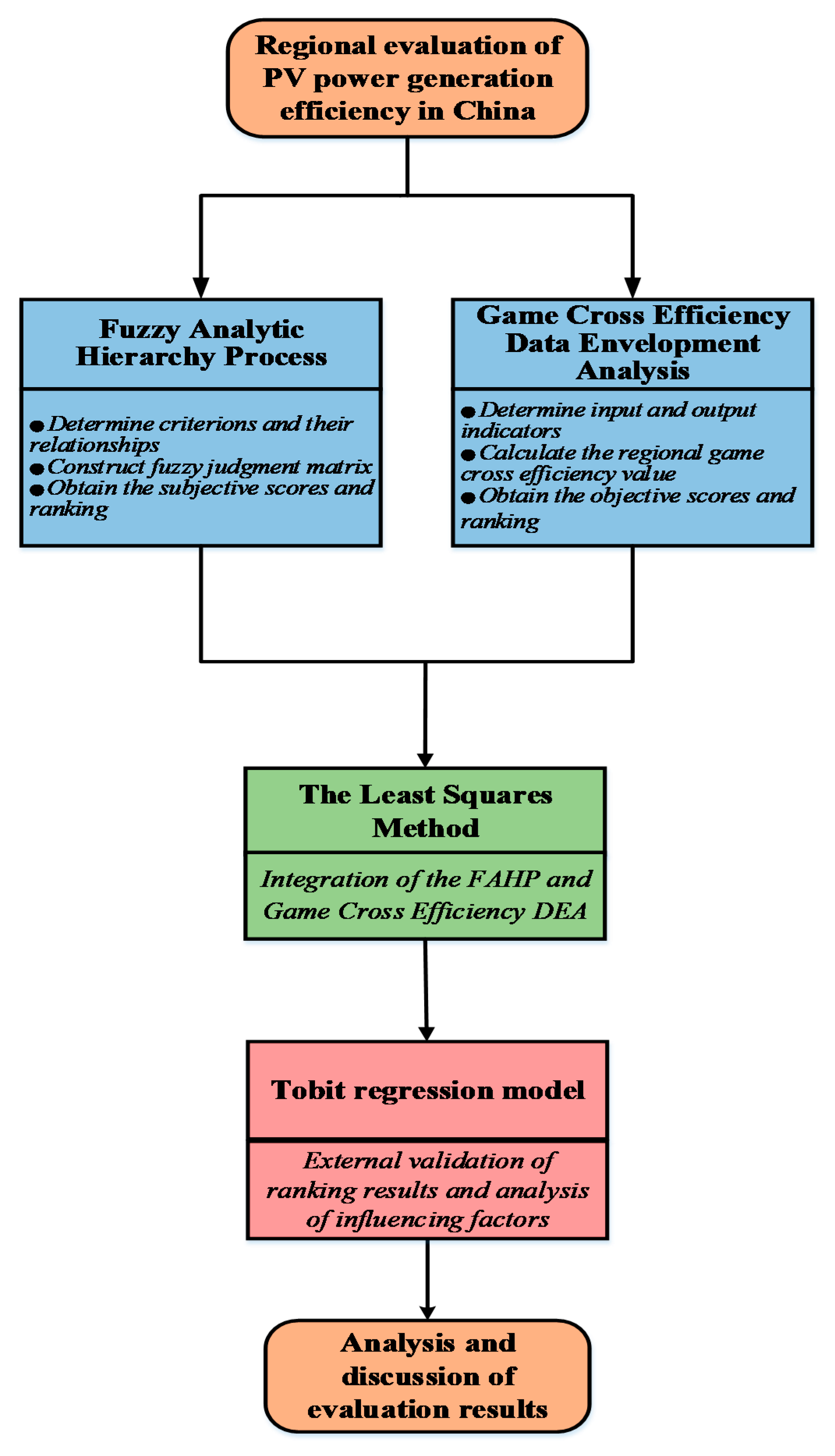
2. Overview of the Methods
2.1. Fuzzy Analytic Hierarchy Process (FAHP)
2.2. Data Envelopment Analysis (DEA)
2.3. Integration of FAHP and DEA
3. Methodology and Data
3.1. Fuzzy Analytic Hierarchy Process
3.2. Game Cross Efficiency DEA
3.3. The Least Squares Method
3.4. Variables and Data
4. Results and Analysis
4.1. Application of FAHP
4.2. Application of Game Cross Efficiency DEA
4.3. Integration Results
5. Influencing Factors
6. Discussion and Conclusions
Author Contributions
Funding
Conflicts of Interest
Appendix A

| Linguistic Variables | Triangle Fuzzy Numbers | Reciprocal Triangular Fuzzy Numbers |
|---|---|---|
| Extremely Strong | (9,9,9) | (1/9,1/9,/1/9) |
| Intermediate | (7,8,9) | (1/9,1/8,/1/7) |
| Very Strong | (6,7,8) | (1/8,/1/7,1/6) |
| Intermediate | (5,6,7) | (1/7,1/6,1/5) |
| Strong | (4,5,6) | (1/6,1/5,1/4) |
| Intermediate | (3,4,5) | (1/5,1/4,1/3) |
| Moderately strong | (2,3,4) | (1/4,1/3,1/2) |
| Intermediate | (1,2,3) | (1/3,1/2,1) |
| Equally strong | (1,1,1) | (1,1,1) |
| Linguistic Variables | Corresponding Triangular Fuzzy Number |
|---|---|
| Very poor | (1,1,3) |
| Poor | (1,3,5) |
| Fair | (3,5,7) |
| Good | (5,7,9) |
| Very good | (7,9,9) |
Appendix B
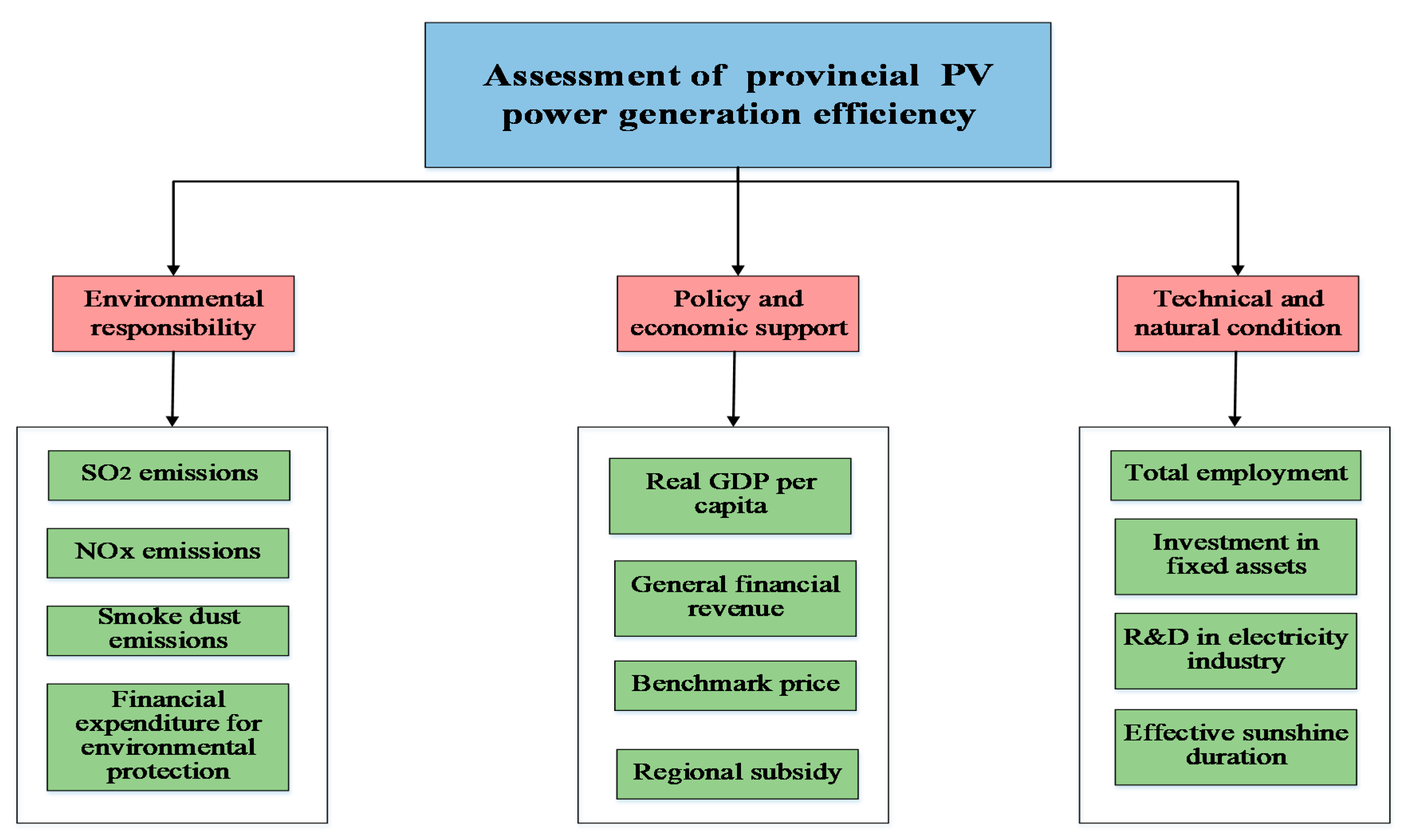
| Criteria | Sub-Criteria | Sub-Criteria Description | References |
|---|---|---|---|
| Environmental responsibility | SO2 emissions | The quality of SO2 emitted by power generation. | [32,33] |
| NOx emissions | The quality of N2O, NO, NO2, N2O3, N2O4 and N2O5 emitted by power generation. | [21,33] | |
| Smoke dust emissions | Quantity of particles with certain size emitted by power generation fuel. | [21,33] | |
| Financial expenditure for environmental protection | Local government expenditure for protecting environment which mainly includes expenditure on environmental monitoring, expenditure on pollution control, expenditure on pollution reduction, etc. | [34,35] | |
| Policy and economic support | Real GDP per capita | Divide the gross domestic product achieved during the accounting period (usually one year) of a country or region by the number of permanent residents of the country or region. | [36,37] |
| General financial revenue | Monetary funds collected by a country or region through certain forms and channels, mainly including various taxes, special income, other income, etc. | [36,38] | |
| Benchmark price | Considering the current cost and reasonable profit of PV power generation, PV power plants sell electricity to grid companies at this price. | [39,40] | |
| Regional subsidy | Relevant financial subsidies invested by local governments to support the development of local PV industry. | [41,42] | |
| Technical and natural conditions | Total employment in electricity industry | Number of people working in the power industry in a certain region. | [1,43] |
| Investment in fixed assets in electricity industry | The amount of work and the costs associated with the construction and acquisition of fixed assets in the power industry for a certain period of time in monetary terms. | [28,38] | |
| R&D in electricity industry | Research and experimental development (R&D) personnel full-time equivalent. | [17,28] | |
| Effective sunshine duration | Number of effective hours of annual illumination calculated from optimum angle of incident light and radiation time. | [44,45] |
Appendix C
| Criteria | Weight | Sub-Criteria | Weight within Criteria | Aggregated Weight |
|---|---|---|---|---|
| Environmental Responsibility | 0.169 | SO2 emissions | 0.2 | 0.034 |
| NOx emissions | 0.2 | 0.034 | ||
| Smoke dust emissions | 0.2 | 0.034 | ||
| Financial expenditure for environmental protection | 0.4 | 0.067 | ||
| Policy and Economic support | 0.388 | Real GDP per capita | 0.125 | 0.049 |
| General financial revenue | 0.365 | 0.142 | ||
| Benchmark price | 0.233 | 0.09 | ||
| Regional subsidy | 0.277 | 0.107 | ||
| Technical and natural condition | 0.443 | Total employment in electricity industry | 0.250 | 0.111 |
| Investment in fixed assets in electricity industry | 0.297 | 0.131 | ||
| R&D in electricity industry | 0.099 | 0.044 | ||
| Effective sunshine duration | 0.354 | 0.157 |
Appendix D
| Criteria | Beijing | Tianjin | Hebei | Shanxi | Inner Mongolia |
|---|---|---|---|---|---|
| SO2 emissions | (233,4.55, 6.52) | (1.25,2.33,4.55) | (2.43,3.90,6.12) | (4.31,6.48,8.39) | (4.86,6.90,8.63) |
| NOx emissions | (2.38,4.53,6.57) | (1.00,2.28,4.40) | (3.56,5.59,7.61) | (2.96,4.69,6.90) | (4.69,6.90,8.39) |
| Smoke dust emissions | (3.39,5.03,7.24) | (1.50,3.34,5.47) | (3.32,5.06,7.19) | (4.69,6.90,8.39) | (3.88,5.13,7.34) |
| Financial expenditure for environmental protection | (2.25,3.76,6.08) | (2.47,3.93,6.25) | (4.19,6.34,8.39) | (3.88,5.13,7.34) | (2.43,3.90,6.12) |
| Real GDP per capita | (5.92,7.94,9.00) | (4.31,6.48,8.39) | (4.69,6.90,8.39) | (3.69,5.32,7.55) | (3.69,5.32,7.55) |
| General financial revenue | (3.66,5.95,7.66) | (3.88,5.13,7.34) | (4.86,6.90,8.63) | (3.22,4.96,7.19) | (3.43,5.59,7.40) |
| Benchmark price | (1.65,3.18,5.39) | (1.00,2.28,4.40) | (3.88,5.13,7.34) | (2.78,4.19,6.43) | (5.36,7.40,8.81) |
| Regional subsidy | (2.96,4.69,6.90) | (1.50,3.34,5.47) | (5.92,7.94,9.00) | (5.36,7.40,8.81) | (4.69,6.90,8.39) |
| Total employment in electricity industry | (2.25,3.76,6.08) | (1.32,2.59,4.79) | (4.40,6.44,8.45) | (4.72,6.76,8.63) | (3.41,5.44,7.45) |
| Investment in fixed assets in electricity industry | (1.72,3.27,5.51) | (2.84,4.56,6.75) | (2.28,4.40,6.44) | (3.53,5.17,7.40) | (4.40,6.44,8.45) |
| R&D in electricity industry | (3.43,5.59,7.40) | (3.41,5.44,7.45) | (3.41,5.44,7.45) | (3.88,5.13,7.34) | (3.69,5.32,7.55) |
| Effective sunshine duration | (2.61,3.93,6.21) | (2.48,4.65,6.71) | (3.69,5.32,7.55) | (4.69,6.90,8.39) | (4.85,6.95,8.28) |
| Criteria | Liaoning | Jilin | Heilongjiang | Shanghai | Jiangsu |
| SO2 emissions | (2.28,4.58,6.48) | (1.25,2.33,4.55) | (1.50,3.34,5.47) | (1.25,2.33,4.55) | (2.94,4.75,6.99) |
| NOx emissions | (2.59,4.79,6.85) | (1.98,4.16,6.21) | (1.65,3.18,5.39) | (1.98,4.16,6.21) | (2.84,4.56,6.75) |
| Smoke dust emissions | (1.32,2.59,4.79) | (2.94,4.75,6.99) | (1.73,3.87,5.92) | (2.47,3.93,6.25) | (3.25,5.36,7.40) |
| Financial expenditure for environmental protection | (2.28,4.40,6.44) | (2.47,3.93,6.25) | (1.00,2.28,4.40) | (3.88,5.13,7.34) | (3.69,5.32,7.55) |
| Real GDP per capita | (1.98,4.16,6.21) | (2.84,4.56,6.75) | (1.25,2.33,4.55) | (5.36,7.40,8.81) | (4.69,6.90,8.39) |
| General financial revenue | (2.94,4.75,6.99) | (2.84,4.56,6.75) | (2.47,3.93,6.25) | (5.92,7.94,9.00) | (4.25,6.43,8.22) |
| Benchmark price | (1.65,3.48,5.63) | (1.72,3.27,5.51) | (1.97,3.51,5.79) | (3.46,5.71,7.66) | (3.18,5.39,7.35) |
| Regional subsidy | (2.42,3.84,6.18) | (3.32,5.55,7.50) | (3.39,5.24,7.29) | (1.98,4.16,6.21) | (4.43,6.61,8.39) |
| Total employment in electricity industry | (2.47,3.93,6.25) | (1.98,4.16,6.21) | (1.25,2.33,4.55) | (3.32,5.06,7.19) | (3.05,4.37,6.61) |
| Investment in fixed assets in electricity industry | (2.94,4.75,6.99) | (2.84,4.56,6.75) | (2.42,3.84,6.18) | (2.07,3.56,5.83) | (3.68,5.87,7.56) |
| R&D in electricity industry | (3.32,5.06,7.19) | (2.96,5.14,7.20) | (2.25,3.76,6.08) | (3.96,6.12,8.05) | (2.84,4.56,6.75) |
| Criteria | Zhejiang | Anhui | Fujian | Jiangxi | Shandong |
| SO2 emissions | (3.69,5.32,7.55) | (5.36,7.40,8.81) | (2.96,5.14,7.20) | (2.42,3.84,6.18) | (3.34,5.47,7.40) |
| NOx emissions | (3.32,5.55,7.50) | (4.31,6.48,8.39) | (3.32,5.06,7.19) | (1.98,4.16,6.21) | (3.39,5.24,7.29) |
| Smoke dust emissions | (3.88,5.13,7.34) | (4.69,6.90,8.39) | (3.88,5.13,7.34) | (3.69,5.32,7.55) | (4.69,6.90,8.39) |
| Financial expenditure for environmental protection | (3.22,4.96,7.19) | (5.92,7.94,9.00) | (3.43,5.59,7.40) | (2.28,4.58,6.48) | (4.86,6.90,8.63) |
| Real GDP per capita | (5.07,7.10,8.81) | (5.36,7.40,8.81) | (3.43,5.59,7.40) | (2.43,3.90,6.12) | (4.40,6.44,8.45) |
| General financial revenue | (4.40,6.44,8.45) | (3.41,5.44,7.45) | (3.69,5.32,7.55) | (3.77,5.03,7.34) | (4.69,6.90,8.39) |
| Benchmark price | (2.94,5.21,7.30) | (3.41,5.44,7.45) | (2.61,3.93,6.21) | (3.69,5.32,7.55) | (5.36,7.40,8.81) |
| Regional subsidy | (5.92,7.94,9.00) | (4.40,6.44,8.45) | (3.88,5.13,7.34) | (2.78,4.19,6.43) | (4.69,6.90,8.39) |
| Total employment in electricity industry | (3.32,5.06,7.19) | (4.19,6.34,8.39) | (3.41,5.44,7.45) | (2.28,4.40,6.44) | (4.40,6.44,8.45) |
| Investment in fixed assets in electricity industry | (3.90,6.08,7.88) | (4.22,6.26,8.28) | (2.78,4.19,6.43) | (2.48,4.65,6.71) | (4.40,6.44,8.45) |
| R&D in electricity industry | (3.41,5.44,7.45) | (5.92,7.94,9.00) | (3.41,5.44,7.45) | (2.28,4.40,6.44) | (3.22,4.96,7.19) |
| Effective sunshine duration | (4.40,6.44,8.45) | (5.92,7.94,9.00) | (4.40,6.44,8.45) | (3.39,5.03,7.24) | (3.41,5.44,7.45) |
| Criteria | Henan | Hubei | Hunan | Guangdong | Guangxi |
| SO2 emissions | (3.34,5.47,7.40) | (4.31,6.48,8.39) | (2.38,4.53,6.57) | (2.33,4.55,6.52) | (2.96,5.14,7.20) |
| NOx emissions | (2.96,4.69,6.90) | (3.77,5.03,7.34) | (2.33,4.55,6.52) | (2.96,4.69,6.90) | (3.32,5.06,7.19) |
| Smoke dust emissions | (3.39,5.03,7.24) | (3.69,5.32,7.55) | (2.25,3.76,6.08) | (4.69,6.90,8.39) | (2.42,3.84,6.18) |
| Financial expenditure for environmental protection | (3.39,5.24,7.29) | (4.69,6.90,8.39) | (2.96,4.69,6.90) | (3.88,5.13,7.34) | (2.33,4.55,6.52) |
| Real GDP per capita | (3.32,5.55,7.50) | (3.69,5.32,7.55) | (3.66,5.95,7.66) | (3.66,5.95,7.66) | (2.96,4.69,6.90) |
| General financial revenue | (3.43,5.59,7.40) | (3.22,4.96,7.19) | (2.38,4.53,6.57) | (5.92,7.94,9.00) | (2.43,3.90,6.12) |
| Benchmark price | (3.88,5.13,7.34) | (2.78,4.19,6.43) | (2.25,3.76,6.08) | (4.40,6.44,8.45) | (2.96,5.14,7.20) |
| Regional subsidy | (3.69,5.32,7.55) | (5.36,7.40,8.81) | (1.65,3.48,5.63) | (4.69,6.90,8.39) | (3.32,5.06,7.19) |
| Total employment in electricity industry | (3.32,5.06,7.19) | (4.86,6.90,8.63) | (2.42,3.84,6.18) | (4.72,6.76,8.63) | (2.25,3.76,6.08) |
| Investment in fixed assets in electricity industry | (3.90,6.08,7.88) | (5.07,7.10,8.81) | (2.47,3.93,6.25) | (3.53,5.17,7.40) | (1.65,3.48,5.63) |
| R&D in electricity industry | (3.41,5.44,7.45) | (3.88,5.13,7.34) | (2.94,4.75,6.99) | (5.36,7.40,8.81) | (3.96,6.12,8.05) |
| Effective sunshine duration | (3.32,5.06,7.19) | (4.69,6.90,8.39) | (2.28,3.66,5.91) | (3.68,5.87,7.56) | (2.07,3.56,5.83) |
| Criteria | Hainan | Chongqing | Sichuan | Guizhou | Yunnan |
| SO2 emissions | (1.65,3.18,5.39) | (1.50,3.34,5.47) | (3.56,5.59,7.61) | (4.85,6.95,8.28) | (3.88,5.13,7.34) |
| NOx emissions | (1.65,3.82,5.87) | (2.48,4.65,6.71) | (2.96,4.69,6.90) | (4.69,6.90,8.39) | (5.36,7.40,8.81) |
| Smoke dust emissions | (1.98,4.16,6.21) | (1.25,2.33,4.55) | (3.34,5.47,7.40) | (4.25,6.43,8.22) | (5.92,7.94,9.00) |
| Financial expenditure for environmental protection | (2.94,4.75,6.99) | (2.47,3.93,6.25) | (3.39,5.24,7.29) | (4.69,6.90,8.39) | (3.32,5.06,7.19) |
| Real GDP per capita | (2.84,4.56,6.75) | (1.72,3.27,5.51) | (3.43,5.59,7.40) | (3.39,5.24,7.29) | (2.47,3.93,6.25) |
| General financial revenue | (2.84,4.56,6.75) | (2.84,4.56,6.75) | (3.32,5.55,7.50) | (4.40,6.44,8.45) | (2.07,3.56,5.83) |
| Benchmark price | (3.32,5.55,7.50) | (1.98,4.16,6.21) | (3.39,5.03,7.24) | (5.36,7.40,8.81) | (1.98,4.16,6.21) |
| Regional subsidy | (2.28,4.40,6.44) | (2.96,5.14,7.20) | (3.32,5.06,7.19) | (3.90,6.08,7.88) | (3.46,5.71,7.66) |
| Total employment in electricity industry | (1.98,4.16,6.21) | (1.32,2.59,4.79) | (3.41,5.44,7.45) | (4.86,6.90,8.63) | (3.34,5.47,7.40) |
| Investment in fixed assets in electricity industry | (2.94,4.75,6.99) | (1.65,3.48,5.63) | (3.32,5.06,7.19) | (4.69,6.90,8.39) | (3.96,6.12,8.05) |
| R&D in electricity industry | (2.42,3.84,6.18) | (2.47,3.93,6.25) | (2.94,4.75,6.99) | (4.69,6.90,8.39) | (3.39,5.24,7.29) |
| Effective sunshine duration | (2.94,4.75,6.99) | (3.32,5.06,7.19) | (2.28,4.40,6.44) | (3.32,5.06,7.19) | (3.39,5.03,7.24) |
| Criteria | Shaanxi | Gansu | Qinghai | Ningxia | Xinjiang |
| SO2 emissions | (3.32,5.06,7.19) | (1.32,2.59,4.79) | (1.98,4.16,6.21) | (2.47,3.93,6.25) | (3.22,4.96,7.19) |
| NOx emissions | (2.61,3.93,6.21) | (2.28,4.58,6.48) | (2.42,3.84,6.18) | (2.28,4.58,6.48) | (2.07,3.56,5.83) |
| Smoke dust emissions | (3.43,5.59,7.40) | (2.28,4.40,6.44) | (1.98,4.16,6.21) | (3.69,5.32,7.55) | (2.47,3.93,6.25) |
| Financial expenditure for environmental protection | (3.69,5.32,7.55) | (2.59,4.79,6.85) | (1.65,3.82,5.87) | (3.77,5.03,7.34) | (3.32,5.06,7.19) |
| Real GDP per capita | (3.41,5.44,7.45) | (1.98,4.16,6.21) | (3.32,5.55,7.50) | (2.43,3.90,6.12) | (2.28,4.40,6.44) |
| General financial revenue | (3.43,5.59,7.40) | (2.47,3.93,6.25) | (2.84,4.56,6.75) | (2.28,4.40,6.44) | (3.88,5.13,7.34) |
| Benchmark price | (3.88,5.13,7.34) | (2.42,3.84,6.18) | (2.94,4.75,6.99) | (2.78,4.19,6.43) | (4.25,6.43,8.22) |
| Regional subsidy | (3.88,5.13,7.34) | (1.65,3.48,5.63) | (2.84,4.56,6.75) | (2.28,4.40,6.44) | (4.69,6.90,8.39) |
| Total employment in electricity industry | (3.43,5.59,7.40) | (2.94,4.75,6.99) | (2.38,4.53,6.57) | (3.69,5.32,7.55) | (2.94,5.21,7.30) |
| Investment in fixed assets in electricity industry | (3.34,5.47,7.40) | (2.94,4.75,6.99) | (2.28,4.40,6.44) | (2.48,4.65,6.71) | (2.61,3.93,6.21) |
| R&D in electricity industry | (3.39,5.24,7.29) | (2.47,3.93,6.25) | (3.39,5.03,7.24) | (3.05,4.37,6.61) | (2.78,4.19,6.43) |
| Effective sunshine duration | (2.96,4.69,6.90) | (2.42,3.84,6.18) | (2.25,3.76,6.08) | (3.32,5.06,7.19) | (5.07,7.10,8.81) |
Appendix E
| Criteria | Beijing | Tianjin | Hebei | Shanxi | Inner Mongolia |
|---|---|---|---|---|---|
| SO2 emissions | 4.47 | 2.71 | 4.15 | 6.39 | 6.80 |
| NOx emissions | 4.49 | 2.56 | 5.59 | 4.85 | 6.66 |
| Smoke dust emissions | 5.22 | 3.44 | 5.19 | 6.66 | 5.45 |
| Financial expenditure for environmental protection | 4.03 | 4.21 | 6.31 | 5.45 | 4.15 |
| Real GDP per capita | 7.62 | 6.39 | 6.66 | 5.52 | 5.52 |
| General financial revenue | 5.76 | 5.45 | 6.80 | 5.12 | 5.47 |
| Benchmark price | 3.41 | 2.56 | 5.45 | 4.46 | 7.19 |
| Regional subsidy | 4.85 | 3.44 | 7.62 | 7.19 | 6.66 |
| Total employment in electricity industry | 4.03 | 2.90 | 6.43 | 6.70 | 5.43 |
| Investment in fixed assets in electricity industry | 3.50 | 4.72 | 4.37 | 5.37 | 6.43 |
| R&D in electricity industry | 5.47 | 5.43 | 5.43 | 5.45 | 5.52 |
| Effective sunshine duration | 4.25 | 4.62 | 5.52 | 6.66 | 6.69 |
| Criteria | Liaoning | Jilin | Heilongjiang | Shanghai | Jiangsu |
| SO2 emissions | 4.45 | 2.71 | 3.44 | 2.71 | 4.90 |
| NOx emissions | 4.74 | 4.12 | 3.41 | 4.12 | 4.72 |
| Smoke dust emissions | 2.90 | 4.90 | 3.84 | 4.21 | 5.34 |
| Financial expenditure for environmental protection | 4.37 | 4.21 | 2.56 | 5.45 | 5.52 |
| Real GDP per capita | 4.12 | 4.72 | 2.71 | 7.19 | 6.66 |
| General financial revenue | 4.90 | 4.72 | 4.21 | 7.62 | 6.30 |
| Benchmark price | 3.59 | 3.50 | 3.75 | 5.61 | 5.31 |
| Regional subsidy | 4.15 | 5.46 | 5.31 | 4.12 | 6.48 |
| Total employment in electricity industry | 4.21 | 4.12 | 2.71 | 5.19 | 4.67 |
| Investment in fixed assets in electricity industry | 4.90 | 4.72 | 4.15 | 3.82 | 5.70 |
| R&D in electricity industry | 5.19 | 5.10 | 4.03 | 6.04 | 4.72 |
| Effective sunshine duration | 5.00 | 6.30 | 5.52 | 5.38 | 6.66 |
| Criteria | Zhejiang | Anhui | Fujian | Jiangxi | Shandong |
| SO2 emissions | 5.52 | 7.19 | 6.30 | 4.15 | 5.40 |
| NOx emissions | 5.46 | 6.39 | 5.19 | 4.12 | 5.31 |
| Smoke dust emissions | 5.45 | 6.66 | 5.45 | 5.52 | 6.66 |
| Financial expenditure for environmental protection | 5.12 | 7.62 | 5.47 | 4.45 | 6.80 |
| Real GDP per capita | 6.99 | 7.19 | 5.47 | 4.15 | 6.43 |
| General financial revenue | 6.43 | 5.43 | 5.52 | 5.38 | 6.66 |
| Benchmark price | 5.15 | 5.43 | 4.25 | 5.52 | 7.19 |
| Regional subsidy | 7.62 | 6.43 | 5.45 | 4.46 | 6.66 |
| Total employment in electricity industry | 5.19 | 6.31 | 5.43 | 4.37 | 6.43 |
| Investment in fixed assets in electricity industry | 5.95 | 6.25 | 4.46 | 4.62 | 6.43 |
| R&D in electricity industry | 5.43 | 7.62 | 5.43 | 4.37 | 5.12 |
| Effective sunshine duration | 6.43 | 7.62 | 6.43 | 5.22 | 5.43 |
| Criteria | Henan | Hubei | Hunan | Guangdong | Guangxi |
| SO2 emissions | 5.40 | 6.39 | 4.49 | 4.47 | 6.30 |
| NOx emissions | 4.85 | 5.38 | 4.47 | 4.85 | 5.19 |
| Smoke dust emissions | 5.22 | 5.52 | 4.03 | 6.66 | 4.15 |
| Financial expenditure for environmental protection | 5.31 | 6.66 | 4.85 | 5.45 | 4.47 |
| Real GDP per capita | 5.46 | 5.52 | 5.76 | 5.76 | 4.85 |
| General financial revenue | 5.47 | 5.12 | 4.49 | 7.62 | 4.15 |
| Benchmark price | 5.45 | 4.46 | 4.03 | 6.43 | 6.30 |
| Regional subsidy | 5.52 | 7.19 | 3.59 | 6.66 | 5.19 |
| Total employment in electricity industry | 5.19 | 6.80 | 4.15 | 6.70 | 4.03 |
| Investment in fixed assets in electricity industry | 5.95 | 6.99 | 4.21 | 5.37 | 3.59 |
| R&D in electricity industry | 5.43 | 5.45 | 4.90 | 7.19 | 6.04 |
| Effective sunshine duration | 5.19 | 6.66 | 3.95 | 5.70 | 3.82 |
| Criteria | Hainan | Chongqing | Sichuan | Guizhou | Yunnan |
| SO2 emissions | 3.41 | 3.44 | 5.59 | 6.69 | 5.45 |
| NOx emissions | 3.78 | 4.62 | 4.85 | 6.66 | 7.19 |
| Smoke dust emissions | 4.12 | 2.71 | 5.40 | 6.30 | 7.62 |
| Financial expenditure for environmental protection | 4.90 | 4.21 | 5.31 | 6.66 | 5.19 |
| Real GDP per capita | 4.72 | 3.50 | 5.47 | 5.31 | 4.21 |
| General financial revenue | 4.72 | 4.72 | 5.46 | 6.43 | 3.82 |
| Benchmark price | 5.46 | 4.12 | 5.22 | 7.19 | 4.12 |
| Regional subsidy | 4.37 | 6.30 | 5.19 | 5.95 | 5.61 |
| Total employment in electricity industry | 4.12 | 2.90 | 5.43 | 6.80 | 5.40 |
| Investment in fixed assets in electricity industry | 4.90 | 3.59 | 5.19 | 6.66 | 6.04 |
| R&D in electricity industry | 4.15 | 4.21 | 4.90 | 6.66 | 5.31 |
| Effective sunshine duration | 4.90 | 5.19 | 4.37 | 5.19 | 5.22 |
| Criteria | Shaanxi | Gansu | Qinghai | Ningxia | Xinjiang |
| SO2 emissions | 5.19 | 2.90 | 4.12 | 4.21 | 5.12 |
| NOx emissions | 4.25 | 4.45 | 4.15 | 4.45 | 3.82 |
| Smoke dust emissions | 5.47 | 4.37 | 4.12 | 5.52 | 4.21 |
| Financial expenditure for environmental protection | 5.52 | 4.74 | 3.78 | 5.38 | 5.19 |
| Real GDP per capita | 5.43 | 4.12 | 5.46 | 4.15 | 4.37 |
| General financial revenue | 5.47 | 4.21 | 4.72 | 4.37 | 5.45 |
| Benchmark price | 5.45 | 4.15 | 4.90 | 4.46 | 6.30 |
| Regional subsidy | 5.45 | 3.59 | 4.72 | 4.37 | 6.66 |
| Total employment in electricity industry | 5.47 | 4.90 | 4.49 | 5.52 | 5.15 |
| Investment in fixed assets in electricity industry | 5.40 | 4.90 | 4.37 | 4.62 | 4.25 |
| R&D in electricity industry | 5.31 | 4.21 | 5.22 | 4.67 | 4.46 |
| Effective sunshine duration | 4.85 | 4.15 | 4.03 | 5.19 | 6.99 |
References
- Guo, X.; Guo, X. China’s photovoltaic power development under policy incentives: A system dynamics analysis. Energy 2015, 93, 589–598. [Google Scholar] [CrossRef]
- Chang, Y.; Gao, L.Q.; Gao, F.G.; Li, F.Z. Benefit Assessment of Solar Photovoltaic Industry in China. Adv. Mater. Res. 2012, 11–16, 608–609. [Google Scholar] [CrossRef]
- Li, N.; Liu, C.; Zha, D. Performance evaluation of Chinese photovoltaic companies with the input-oriented dynamic SBM model. Renew. Energy 2016, 89, 489–497. [Google Scholar] [CrossRef]
- Yang, J.; Yang, C.; Song, Y.; Wang, X. Exploring Promotion Effect for FIT Policy of Solar PV Power Generation Based on Integrated ANP: Entropy Model. Math. Probl. Eng. 2018, 2018, 7176059. [Google Scholar] [CrossRef]
- Saaty, T.L.; Peniwati, K.; Shang, J.S. The analytic hierarchy process and human resource allocation: Half the story. Math. Comput. Model. 2007, 46, 1041–1053. [Google Scholar] [CrossRef]
- Chan, F.T.S.; Kumar, N. Global supplier development considering risk factors using fuzzy extended AHP-based approach. Omega 2007, 35, 417–431. [Google Scholar] [CrossRef]
- Lee, A.H.I.; Chen, W.-C.; Chang, C.-J. A fuzzy AHP and BSC approach for evaluating performance of IT department in the manufacturing industry in Taiwan. Expert Syst. Appl. 2008, 34, 96–107. [Google Scholar] [CrossRef]
- Balusa, B.C.; Gorai, A.K. Sensitivity analysis of fuzzy-analytic hierarchical process (FAHP) decision-making model in selection of underground metal mining method. J. Sustain. Min. 2019, 18, 8–17. [Google Scholar] [CrossRef]
- He, Y.; Du, S. Classification of Urban Emergency Based on Fuzzy Analytic Hierarchy Process. Procedia Eng. 2016, 137, 630–638. [Google Scholar] [CrossRef] [Green Version]
- Jakiel, P.; Fabianowski, D. FAHP model used for assessment of highway RC bridge structural and technological arrangements. Expert Syst. Appl. 2015, 42, 4054–4061. [Google Scholar] [CrossRef]
- Geng, Z.; Qin, L.; Han, Y.; Zhu, Q. Energy saving and prediction modeling of petrochemical industries: A novel ELM based on FAHP. Energy 2017, 122, 350–362. [Google Scholar] [CrossRef]
- Chames, A.; Cooper, W.W.; Rhodes, E. Measuring the efficiency of decision making units. Eur. J. Oper. Res. 1978, 2, 429–444. [Google Scholar]
- Borozan, D. Technical and total factor energy efficiency of European regions: A two-stage approach. Energy 2018, 152, 521–532. [Google Scholar] [CrossRef]
- Rybaczewska-Błażejowska, M.; Masternak-Janus, A. Eco-efficiency assessment of Polish regions: Joint application of life cycle assessment and data envelopment analysis. J. Clean. Prod. 2018, 172, 1180–1192. [Google Scholar] [CrossRef]
- Kounetas, K.; Napolitano, O. Modeling the incidence of international trade on Italian regional productive efficiency using a meta-frontier DEA approach. Econ. Model. 2018, 71, 45–58. [Google Scholar] [CrossRef]
- Yang, G.-l.; Fukuyama, H.; Chen, K. Investigating the regional sustainable performance of the Chinese real estate industry: A slack-based DEA approach. Omega 2019, 84, 141–159. [Google Scholar] [CrossRef]
- Chen, K.; Kou, M.; Fu, X. Evaluation of multi-period regional R&D efficiency: An application of dynamic DEA to China’s regional R&D systems. Omega 2018, 74, 103–114. [Google Scholar]
- Hadi-Vencheh, A.; Mohamadghasemi, A. A fuzzy AHP-DEA approach for multiple criteria ABC inventory classification. Expert Syst. Appl. 2011, 38, 3346–3352. [Google Scholar] [CrossRef]
- Che, Z.H.; Wang, H.S.; Chuang, C.-L. A fuzzy AHP and DEA approach for making bank loan decisions for small and medium enterprises in Taiwan. Expert Syst. Appl. 2010, 37, 7189–7199. [Google Scholar] [CrossRef]
- Li, X.; Liu, Y.; Wang, Y.; Gao, Z. Evaluating transit operator efficiency: An enhanced DEA model with constrained fuzzy-AHP cones. J. Traffic Transp. Eng. (Engl. Ed.) 2016, 3, 215–225. [Google Scholar] [CrossRef] [Green Version]
- Shen, Y.-C.; Lin, G.T.R.; Li, K.-P.; Yuan, B.J.C. An assessment of exploiting renewable energy sources with concerns of policy and technology. Energy Policy 2010, 38, 4604–4616. [Google Scholar] [CrossRef]
- Chen, C.T. Extensions of TOPSIS for group decision-making under fuzzy environment. Fuzzy Sets Syst. 2000, 114, 1–9. [Google Scholar] [CrossRef]
- Liang, L.; Wu, J.; Cook, W.D.; Zhu, J. Alternative secondary goals in DEA cross-efficiency evaluation. Int. J. Prod. Econ. 2008, 113, 1025–1030. [Google Scholar] [CrossRef]
- Liang, L.; Wu, J.; Cook, W.D.; Zhu, J. The DEA Game Cross-Efficiency Model and Its Nash Equilibrium. Oper. Res. 2008, 56, 1278–1288. [Google Scholar] [CrossRef] [Green Version]
- Wang, Z.; Li, Y.; Wang, K.; Huang, Z. Environment-adjusted operational performance evaluation of solar photovoltaic power plants: A three stage efficiency analysis. Renew. Sustain. Energy Rev. 2017, 76, 1153–1162. [Google Scholar] [CrossRef]
- Honrubia-Escribano, A.; Ramirez, F.J.; Gómez-Lázaro, E.; Garcia-Villaverde, P.M.; Ruiz-Ortega, M.J.; Parra-Requena, G. Influence of solar technology in the economic performance of PV power plants in Europe. A comprehensive analysis. Renew. Sustain. Energy Rev. 2018, 82, 488–501. [Google Scholar] [CrossRef]
- Chien, T.; Hu, J.-L. Renewable energy and macroeconomic efficiency of OECD and non-OECD economies. Energy Policy 2007, 35, 3606–3615. [Google Scholar] [CrossRef]
- Li, L.; Chi, T.; Zhang, M.; Wang, S. Multi-Layered Capital Subsidy Policy for the PV Industry in China Considering Regional Differences. Sustainability 2016, 8, 45. [Google Scholar] [CrossRef] [Green Version]
- Opricovic, S.; Tzeng, G.H. Defuzzification within a multicriteria decision model. Int. J. Uncertain. Fuzziness Knowl. Based Syst. 2003, 11, 635–652. [Google Scholar] [CrossRef]
- Sueyoshi, T.; Goto, M. Photovoltaic power stations in Germany and the United States: A comparative study by data envelopment analysis. Energy Econ. 2014, 42, 271–288. [Google Scholar] [CrossRef]
- Sueyoshi, T.; Goto, M. Can environmental investment and expenditure enhance financial performance of US electric utility firms under the clean air act amendment of 1990? Energy Policy 2009, 37, 4819–4826. [Google Scholar] [CrossRef]
- Komor, P.; Bazilian, M. Renewable energy policy goals, programs, and technologies. Energy Policy 2005, 33, 1873–1881. [Google Scholar] [CrossRef]
- Begić, F.; Afgan, N.H. Sustainability assessment tool for the decision making in selection of energy system—Bosnian case. Energy 2007, 32, 1979–1985. [Google Scholar] [CrossRef]
- Kaldellis, J.K.; Fragos, P.; Kapsali, M. Systematic experimental study of the pollution deposition impact on the energy yield of photovoltaic installations. Renew. Energy 2011, 36, 2717–2724. [Google Scholar] [CrossRef]
- Kaldellis, J.K.; Kapsali, M. Simulating the dust effect on the energy performance of photovoltaic generators based on experimental measurements. Energy 2011, 36, 5154–5161. [Google Scholar] [CrossRef]
- Ren, H.; Zhou, W.; Nakagami, K.i.; Gao, W.; Wu, Q. Multi-objective optimization for the operation of distributed energy systems considering economic and environmental aspects. Appl. Energy 2010, 87, 3642–3651. [Google Scholar] [CrossRef]
- Alper, A.; Oguz, O. The role of renewable energy consumption in economic growth: Evidence from asymmetric causality. Renew. Sustain. Energy Rev. 2016, 60, 953–959. [Google Scholar] [CrossRef]
- Hossein, S.S.M.; Yazdan, G.F.; Hasan, S. Consideration the Relationship between Energy Consumption and Economic Growth in Oil Exporting Country. Procedia Soc. Behav. Sci. 2012, 62, 52–58. [Google Scholar] [CrossRef] [Green Version]
- Jeon, C.; Lee, J.; Shin, J. Optimal subsidy estimation method using system dynamics and the real option model: Photovoltaic technology case. Appl. Energy 2015, 142, 33–43. [Google Scholar] [CrossRef]
- Macintosh, A.; Wilkinson, D. Searching for public benefits in solar subsidies: A case study on the Australian government’s residential photovoltaic rebate program. Energy Policy 2011, 39, 3199–3209. [Google Scholar] [CrossRef]
- Rigter, J.; Vidican, G. Cost and optimal feed-in tariff for small scale photovoltaic systems in China. Energy Policy 2010, 38, 6989–7000. [Google Scholar] [CrossRef]
- Sun, H.; Zhi, Q.; Wang, Y.; Yao, Q.; Su, J. China’s solar photovoltaic industry development: The status quo, problems and approaches. Appl. Energy 2014, 118, 221–230. [Google Scholar] [CrossRef]
- Gao, L.Q.; Chang, Y.; Li, B.Y.; Li, F.Z. The Analysis of Chinese Photovoltaic Industry with SWOT Model and AHP Method. Adv. Mater. Res. 2012, 608–609, 137–142. [Google Scholar] [CrossRef]
- Mondal, M.A.H.; Islam, A.K.M.S. Potential and viability of grid-connected solar PV system in Bangladesh. Renew. Energy 2011, 36, 1869–1874. [Google Scholar] [CrossRef]
- Sheikh, M.A. Renewable energy resource potential in Pakistan. Renew. Sustain. Energy Rev. 2009, 13, 2696–2702. [Google Scholar] [CrossRef]


| Type of Analysis | Type of Variables | Variables |
|---|---|---|
| FAHP (subjective analysis) | (criteria) Environmental responsibility | (sub-criteria) SO2 emissions |
| NOx emissions | ||
| smoke dust emissions | ||
| financial expenditure for environmental protection | ||
| Policy and economic support | real GDP per capita | |
| general financial revenue | ||
| benchmark price | ||
| regional subsidy | ||
| Technical and natural condition | total employment | |
| investment in fixed assets | ||
| R&D in electricity industry | ||
| effective sunshine duration | ||
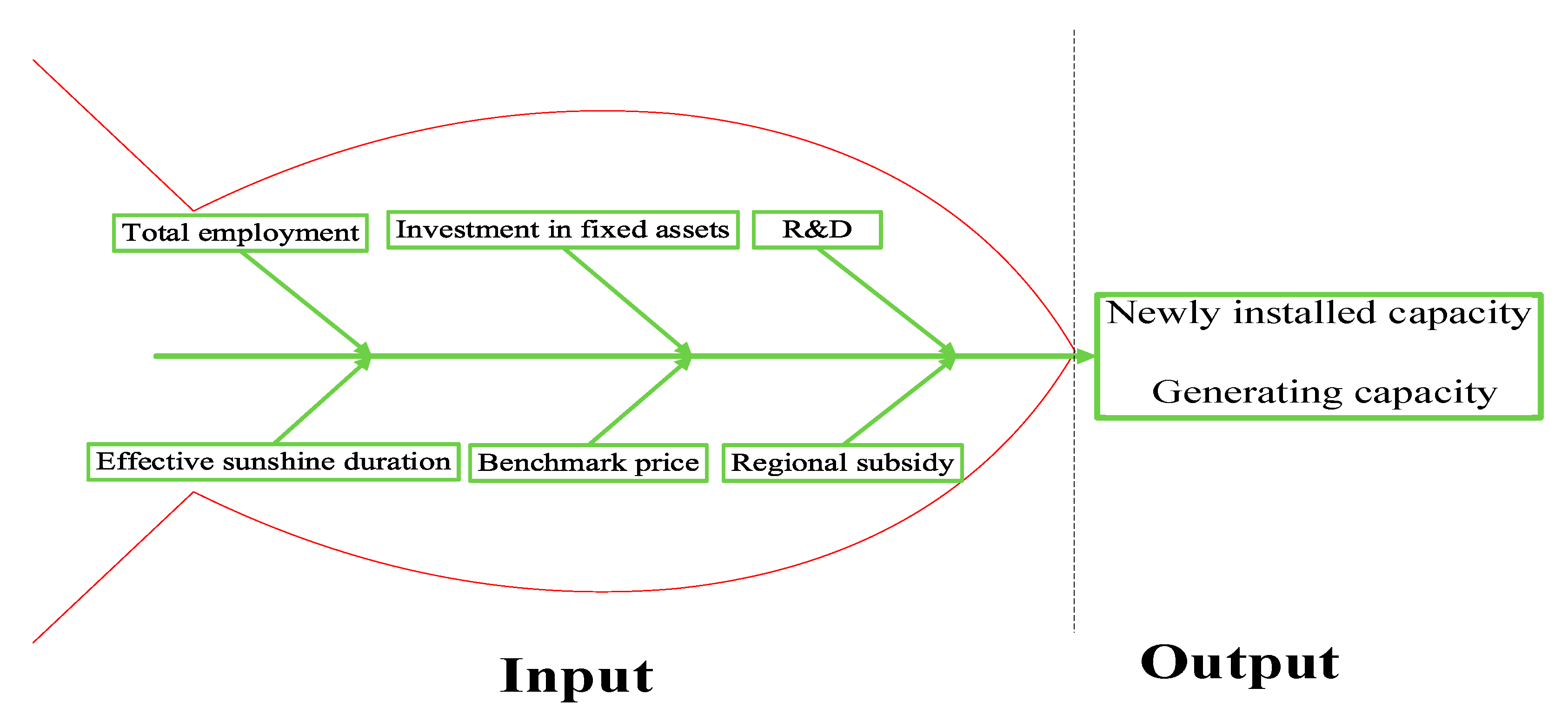
| Game cross efficiency DEA (objective analysis) | Input variables | total employment |
| investment in fixed assets | ||
| R&D in electricity industry | ||
| effective sunshine duration | ||
| benchmark price | ||
| regional subsidy | ||
| Output variables | new installed capacity | |
| generating capacity | ||
| Tobit Regression (Outside validation) | Independent variables | real GDP per capita |
| general financial revenue | ||
| electricity consumption | ||
| total energy consumption per unit GDP | ||
| financial expenditure for environmental protection | ||
| NOx emissions | ||
| SO2 emissions | ||
| smoke dust emissions | ||
| R&D in electricity industry | ||
| Dependent variable | comprehensive efficiency scores |
| Variable | Mean | Minimum | Maximum | Standard Deviation |
|---|---|---|---|---|
| SO2 emissions (Ton) | 523,563.35 | 14,271.49 | 1,644,967.09 | 362,319.81 |
| NOx emissions (Ton) | 585,763.32 | 60,132.01 | 1,652,467.63 | 379,762.88 |
| smoke dust emissions (Ton) | 423,849.98 | 18,003.18 | 1,797,683.42 | 335,809.43 |
| financial expenditure for environmental protection (100 Million Yuan) | 138.21 | 23.18 | 458.44 | 78.62 |
| real GDP per capita (Yuan/Capita) | 24,422.98 | 2122.06 | 89,705.23 | 18,528.36 |
| general financial revenue (100 Million Yuan) | 2706.01 | 223.86 | 11,320.35 | 2087.94 |
| benchmark price (Yuan) | 0.86 | 0.55 | 1 | 0.13 |
| regional subsidy (Yuan) | 0.45 | 0 | 1 | 0.49 |
| total employment (10 Thousand people) | 13.09 | 1.85 | 32.18 | 6.97 |
| investment in fixed assets (100 Million Yuan) | 845.79 | 107.24 | 2886.91 | 522.13 |
| R&D in electricity industry (Man year) | 88,079.34 | 1285 | 457,342 | 113,056.36 |
| effective sunshine duration (Hour) | 1212.77 | 686.27 | 1699.65 | 226.09 |
| new installed capacity (10 thousand kW) | 83.26 | 0.2 | 597 | 113.55 |
| generating capacity (100 Million kWh) | 1950.59 | 230.74 | 5329.27 | 1222.35 |
| electricity consumption (100 Million kWh) | 1924.03 | 232 | 5958.97 | 1344.47 |
| total energy consumption per unit GDP (Tons of standard coal/10 Thousand Yuan) | 0.76 | 0.25 | 2.17 | 0.41 |
| Regions | Scores | Normalized Scores | Rankings |
|---|---|---|---|
| Beijing | 4.58304 | 0. 4583 | 22 |
| Tianjin | 4.16818 | 0.4168 | 29 |
| Hebei | 5.91993 | 0.5920 | 8 |
| Shanxi | 5.87459 | 0.5875 | 9 |
| Inner Mongolia | 6.0662 | 0.6066 | 6 |
| Liaoning | 4.49125 | 0.4491 | 25 |
| Jilin | 4.77077 | 0.4771 | 20 |
| Heilongjiang | 4.05968 | 0.4060 | 30 |
| Shanghai | 5.30753 | 0.5308 | 14 |
| Jiangsu | 5.78905 | 0.5789 | 10 |
| Zhejiang | 6.04004 | 0.6040 | 7 |
| Anhui | 6.54956 | 0.6550 | 1 |
| Fujian | 5.39539 | 0.5395 | 13 |
| Jiangxi | 4.81045 | 0.4810 | 18 |
| Shandong | 6.30054 | 0.6301 | 3 |
| Henan | 5.41646 | 0.5416 | 12 |
| Hubei | 6.15824 | 0.6158 | 5 |
| Hunan | 4.28117 | 0.4281 | 28 |
| Guangdong | 6.2225 | 0.6223 | 4 |
| Guangxi | 4.56365 | 0.4564 | 23 |
| Hainan | 4.62447 | 0.4624 | 21 |
| Chongqing | 4.32715 | 0.4327 | 26 |
| Sichuan | 5.14712 | 0.5147 | 17 |
| Guizhou | 6.30645 | 0.6306 | 2 |
| Yunnan | 5.20019 | 0.5200 | 16 |
| Shaanxi | 5.3029 | 0.5303 | 15 |
| Gansu | 4.29598 | 0.4296 | 27 |
| Qinghai | 4.49159 | 0.4492 | 24 |
| Ningxia | 4.77371 | 0.4774 | 19 |
| Xinjiang | 5.48455 | 0.5485 | 11 |
| Regions | 2013 | 2014 | 2015 | 2016 | 2017 |
|---|---|---|---|---|---|
| Beijing | 0.3096 | 0.2770 | 0.0000 | 0.0000 | 0.0000 |
| Tianjin | 0.4741 | 0.5854 | 0.5764 | 0.5821 | 0.4733 |
| Hebei | 1.0000 | 1.0000 | 1.0000 | 1.0000 | 1.0000 |
| Shanxi | 1.0000 | 0.9750 | 1.0000 | 0.9456 | 1.0000 |
| Inner Mongolia | 1.0000 | 1.0000 | 1.0000 | 1.0000 | 1.0000 |
| Liaoning | 0.5464 | 0.6447 | 0.8460 | 1.0000 | 0.8175 |
| Jilin | 0.3887 | 0.4124 | 0.4045 | 0.3768 | 1.0000 |
| Heilongjiang | 0.4146 | 0.4735 | 0.5846 | 0.5179 | 0.5231 |
| Shanghai | 1.0000 | 1.0000 | 1.0000 | 1.0000 | 1.0000 |
| Jiangsu | 1.0000 | 1.0000 | 1.0000 | 1.0000 | 1.0000 |
| Zhejiang | 1.0000 | 1.0000 | 1.0000 | 1.0000 | 0.9714 |
| Anhui | 1.0000 | 1.0000 | 1.0000 | 1.0000 | 1.0000 |
| Fujian | 1.0000 | 1.0000 | 0.9798 | 0.9444 | 1.0000 |
| Jiangxi | 0.5195 | 1.0000 | 0.9976 | 1.0000 | 0.9877 |
| Shandong | 1.0000 | 1.0000 | 1.0000 | 1.0000 | 1.0000 |
| Henan | 1.0000 | 1.0000 | 0.9635 | 0.9223 | 0.9397 |
| Hubei | 0.9922 | 1.0000 | 1.0000 | 1.0000 | 1.0000 |
| Hunan | 0.6188 | 0.5331 | 0.9473 | 1.0000 | 0.9874 |
| Guangdong | 1.0000 | 1.0000 | 1.0000 | 1.0000 | 1.0000 |
| Guangxi | 0.7739 | 0.7656 | 1.0000 | 1.0000 | 1.0000 |
| Hainan | 0.4624 | 0.5223 | 0.6526 | 0.7578 | 1.0000 |
| Chongqing | 0.3946 | 0.4708 | 0.4988 | 0.4527 | 1.0000 |
| Sichuan | 1.0000 | 1.0000 | 1.0000 | 1.0000 | 1.0000 |
| Guizhou | 1.0000 | 1.0000 | 1.0000 | 1.0000 | 1.0000 |
| Yunnan | 1.0000 | 1.0000 | 1.0000 | 1.0000 | 1.0000 |
| Shaanxi | 0.6343 | 1.0000 | 1.0000 | 1.0000 | 1.0000 |
| Gansu | 1.0000 | 1.0000 | 1.0000 | 1.0000 | 1.0000 |
| Qinghai | 1.0000 | 1.0000 | 1.0000 | 0.8992 | 0.7875 |
| Ningxia | 1.0000 | 1.0000 | 1.0000 | 1.0000 | 1.0000 |
| Xinjiang | 1.0000 | 1.0000 | 1.0000 | 1.0000 | 1.0000 |
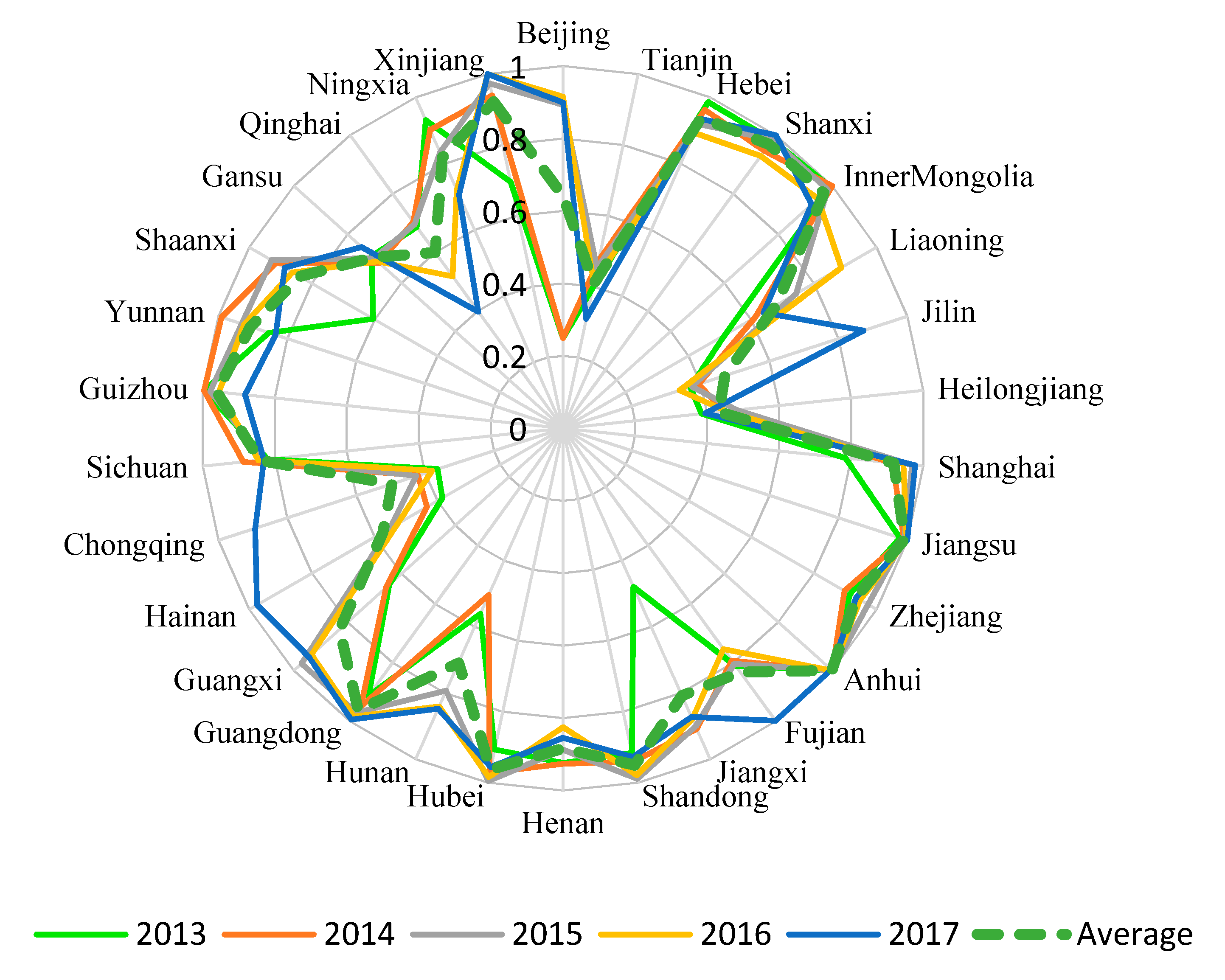
| Regions | 2013 | 2014 | 2015 | 2016 | 2017 | Average |
|---|---|---|---|---|---|---|
| Beijing | 0.2488 | 0.2487 | 0.8928 | 0.9152 | 0.8994 | 0.6410 |
| Tianjin | 0.3978 | 0.4723 | 0.4524 | 0.4104 | 0.3091 | 0.4084 |
| Hebei | 0.9862 | 0.9627 | 0.9194 | 0.8927 | 0.9349 | 0.9392 |
| Shanxi | 0.9839 | 0.9469 | 0.9851 | 0.9294 | 1.0000 | 0.9691 |
| Inner Mongolia | 0.9947 | 1.0000 | 0.9841 | 0.9472 | 0.9235 | 0.9699 |
| Liaoning | 0.5163 | 0.6136 | 0.7432 | 0.8873 | 0.6391 | 0.6799 |
| Jilin | 0.3701 | 0.3937 | 0.374 | 0.3384 | 0.8731 | 0.4699 |
| Heilongjiang | 0.3851 | 0.4463 | 0.4826 | 0.4535 | 0.3952 | 0.4325 |
| Shanghai | 0.7847 | 0.9153 | 0.9693 | 0.9457 | 0.9777 | 0.9185 |
| Jiangsu | 0.9782 | 0.9897 | 0.9906 | 0.9979 | 1.0000 | 0.9913 |
| Zhejiang | 0.9149 | 0.8974 | 0.973 | 0.9473 | 0.9348 | 0.9335 |
| Anhui | 1.0000 | 1.0000 | 1.0000 | 0.9994 | 0.9961 | 0.9991 |
| Fujian | 0.8114 | 0.7929 | 0.8042 | 0.7533 | 0.9983 | 0.8320 |
| Jiangxi | 0.4795 | 0.9084 | 0.9011 | 0.8784 | 0.8726 | 0.8080 |
| Shandong | 0.9163 | 0.9406 | 0.9896 | 0.979 | 0.9279 | 0.9507 |
| Henan | 0.9239 | 0.9268 | 0.8872 | 0.8255 | 0.8545 | 0.8836 |
| Hubei | 0.9067 | 0.9717 | 0.9952 | 0.9844 | 0.9563 | 0.9629 |
| Hunan | 0.5599 | 0.5038 | 0.7933 | 0.8405 | 0.8475 | 0.7090 |
| Guangdong | 0.9131 | 0.9493 | 0.9704 | 0.9831 | 0.9943 | 0.9620 |
| Guangxi | 0.6445 | 0.6576 | 0.9711 | 0.9343 | 0.9438 | 0.8303 |
| Hainan | 0.3844 | 0.4332 | 0.5515 | 0.5269 | 0.9752 | 0.5742 |
| Chongqing | 0.3641 | 0.4208 | 0.4259 | 0.3797 | 0.8931 | 0.4967 |
| Sichuan | 0.8192 | 0.8873 | 0.8278 | 0.8452 | 0.8298 | 0.8419 |
| Guizhou | 0.9961 | 0.996 | 0.979 | 0.9549 | 0.8827 | 0.9617 |
| Yunnan | 0.8537 | 0.991 | 0.9326 | 0.926 | 0.8339 | 0.9074 |
| Shaanxi | 0.6045 | 0.9145 | 0.9287 | 0.8618 | 0.8872 | 0.8393 |
| Gansu | 0.7099 | 0.6824 | 0.701 | 0.6884 | 0.7479 | 0.7059 |
| Qinghai | 0.6863 | 0.7035 | 0.697 | 0.5182 | 0.3975 | 0.6005 |
| Ningxia | 0.9314 | 0.9018 | 0.834 | 0.7204 | 0.7052 | 0.8186 |
| Xinjiang | 0.6954 | 0.9395 | 0.9737 | 1.0000 | 1.0000 | 0.9217 |
| Average | 0.7254 | 0.7803 | 0.8310 | 0.8088 | 0.8477 | 0.7986 |
| Regions | FAHP Scores | DEA Scores | Averaged Scores | Rankings |
|---|---|---|---|---|
| Beijing | 0.4583 | 0.6410 | 0.5497 | 24 |
| Tianjin | 0.4168 | 0.4084 | 0.4126 | 30 |
| Hebei | 0.5920 | 0.9392 | 0.7656 | 10 |
| Shanxi | 0.5875 | 0.9691 | 0.7783 | 8 |
| Inner Mongolia | 0.6066 | 0.9699 | 0.7883 | 6 |
| Liaoning | 0.4491 | 0.6799 | 0.5645 | 23 |
| Jilin | 0.4771 | 0.4699 | 0.4735 | 27 |
| Heilongjiang | 0.4060 | 0.4325 | 0.4193 | 29 |
| Shanghai | 0.5308 | 0.9185 | 0.7247 | 12 |
| Jiangsu | 0.5789 | 0.9913 | 0.7851 | 7 |
| Zhejiang | 0.6040 | 0.9335 | 0.7688 | 9 |
| Anhui | 0.6550 | 0.9991 | 0.8271 | 1 |
| Fujian | 0.5395 | 0.8320 | 0.6858 | 15 |
| Jiangxi | 0.4810 | 0.8080 | 0.6445 | 19 |
| Shandong | 0.6301 | 0.9507 | 0.7904 | 4 |
| Henan | 0.5416 | 0.8836 | 0.7126 | 14 |
| Hubei | 0.6158 | 0.9629 | 0.7894 | 5 |
| Hunan | 0.4281 | 0.7090 | 0.5686 | 21 |
| Guangdong | 0.6223 | 0.9620 | 0.7922 | 3 |
| Guangxi | 0.4564 | 0.8303 | 0.6434 | 20 |
| Hainan | 0.4624 | 0.5742 | 0.5183 | 26 |
| Chongqing | 0.4327 | 0.4967 | 0.4647 | 28 |
| Sichuan | 0.5147 | 0.8419 | 0.6783 | 17 |
| Guizhou | 0.6306 | 0.9617 | 0.7962 | 2 |
| Yunnan | 0.5200 | 0.9074 | 0.7137 | 13 |
| Shaanxi | 0.5303 | 0.8393 | 0.6848 | 16 |
| Gansu | 0.4296 | 0.7059 | 0.5678 | 22 |
| Qinghai | 0.4492 | 0.6005 | 0.5249 | 25 |
| Ningxia | 0.4774 | 0.8186 | 0.6480 | 18 |
| Xinjiang | 0.5485 | 0.9217 | 0.7351 | 11 |
| Mean | 0.5224 | 0.7986 | 0.6605 | - |
| Regions | Comprehensive Scores | Geographic Location | Mean Value | Rankings |
|---|---|---|---|---|
| Beijing | 0.5497 | North China | 0.6589 | 4 |
| Tianjin | 0.4126 | |||
| Hebei | 0.7656 | |||
| Shanxi | 0.7783 | |||
| Inner Mongolia | 0.7883 | |||
| Liaoning | 0.5645 | Northeast China | 0.4858 | 6 |
| Jilin | 0.4735 | |||
| Heilongjiang | 0.4193 | |||
| Shanghai | 0.7247 | East China | 0.7466 | 1 |
| Jiangsu | 0.7851 | |||
| Zhejiang | 0.7688 | |||
| Anhui | 0.8271 | |||
| Fujian | 0.6858 | |||
| Jiangxi | 0.6445 | |||
| Shandong | 0.7904 | |||
| Henan | 0.7126 | Central South China | 0.6707 | 2 |
| Hubei | 0.7894 | |||
| Hunan | 0.5686 | |||
| Guangdong | 0.7922 | |||
| Guangxi | 0.6434 | |||
| Hainan | 0.5183 | |||
| Chongqing | 0.4647 | Southwest China | 0.6632 | 3 |
| Sichuan | 0.6783 | |||
| Guizhou | 0.7962 | |||
| Yunnan | 0.7137 | |||
| Shaanxi | 0.6848 | Northwest China | 0.6321 | 5 |
| Gansu | 0.5678 | |||
| Qinghai | 0.5249 | |||
| Ningxia | 0.6480 | |||
| Xinjiang | 0.7351 |
| Variables | Coefficients | Standard Deviation | P | [Confidence Interval] |
|---|---|---|---|---|
| real GDP per capita (X1) | 0.0898 | 0.0418 | 0.033 ** | [0.0072, 0.1726] |
| general financial revenue (X2) | 0.1391 | 0.0594 | 0.021 ** | [0.0217, 0.2565] |
| electricity consumption (X3) | 0.1085 | 0.0385 | 0.206 | [0.0323, 0.1846] |
| total energy consumption per unit GDP (X4) | −0.0568 | 0.0544 | 0.006 *** | [−0.1644, 0.0508] |
| financial expenditure for environmental protection (X5) | 0.2250 | 0.1344 | 0.096 * | [0.0984, 0.3533] |
| NOx emissions (X6) | −0.2758 | 0.0324 | 0.000 *** | [−0.3399, −0.2116] |
| SO2 emissions (X7) | −0.0063 | 0.0032 | 0.053 * | [−0.0127, 0.0002] |
| smoke dust emissions (X8) | −0.0146 | 0.0327 | 0.095 * | [−0.0974, 0.1194] |
| R&D in electricity industry (X9) | 0.2467 | 0.5788 | 0.323 | [−0.8973, 1.3908] |
© 2020 by the authors. Licensee MDPI, Basel, Switzerland. This article is an open access article distributed under the terms and conditions of the Creative Commons Attribution (CC BY) license (http://creativecommons.org/licenses/by/4.0/).
Share and Cite
Yang, J.; Yang, C.; Wang, X.; Cheng, M.; Shang, J. Efficiency Measurement and Factor Analysis of China’s Solar Photovoltaic Power Generation Considering Regional Differences Based on a FAHP–DEA Model. Energies 2020, 13, 1936. https://doi.org/10.3390/en13081936
Yang J, Yang C, Wang X, Cheng M, Shang J. Efficiency Measurement and Factor Analysis of China’s Solar Photovoltaic Power Generation Considering Regional Differences Based on a FAHP–DEA Model. Energies. 2020; 13(8):1936. https://doi.org/10.3390/en13081936
Chicago/Turabian StyleYang, Jing, Changhui Yang, Xiaojia Wang, Manli Cheng, and Jingjing Shang. 2020. "Efficiency Measurement and Factor Analysis of China’s Solar Photovoltaic Power Generation Considering Regional Differences Based on a FAHP–DEA Model" Energies 13, no. 8: 1936. https://doi.org/10.3390/en13081936