Abstract
This paper applies a heuristic approach to optimize the predictor variables in artificial neural networks when forecasting raw material prices for energy production (coking coal, natural gas, crude oil and coal) to achieve a better forecast. Two goals are (1) to determine the optimum number of time-delayed terms or past values forming the lagged variables and (2) to improve the forecast accuracy by adding intrinsic signals to the lagged variables. The conclusions clearly are in opposition to the actual scientific literature: when addressing the lagged variable size, the results do not confirm relationships among their size, representativeness and estimation accuracy. It is also possible to verify an important effect of the results on the lagged variable size. Finally, adding the order in the time series of the lagged variables to form the predictor variables improves the forecast accuracy in most cases.
1. Introduction
Artificial neural networks (ANN) have been widely used as accurate forecast aids addressing issues directly or indirectly related with energy or raw materials: energy production [1], raw material inventory levels [2], crude oil prices [3], volatility of stock price indices [4], electricity prices [5], stock prices [6], gold prices [7], copper spot prices [8], off-gases production [9], currency exchange rates [10], etc.
This paper analyzes the forecast of raw material prices for energy production by means of ANN, focusing on the selection of optimum parameters in order to configure the ANN. Design of experiments (DOE) is normally used to select these parameters [11].
DOE can be focused on estimating the number of neurons in hidden layers [12], on forming training and test datasets [13], on eliminating redundant dimensions in the predictor variables trying to achieve compression [14,15], on determining the optimum size of the lagged variables [16], on adding signals to the lagged variables [17], etc.
A heuristic approach will be used to optimize the predictor variables in ANN by means of (1) modifying the lagged variable size and (2) adding intrinsic signals to the lagged variables.
Addressing the lagged variable size, Liu and Su [18] indicated that a larger size allows for increasing the forecast accuracy, while it decreases the representativeness of the subsample heterogeneity. Moreover, although smaller sizes may improve representativeness, they will reduce the estimation accuracy. In the above empirical research, they used lagged variable sizes of 12, 24 and 36 months to test different alternatives. Nevertheless, the lagged variable sizes indicate very little effect on the results.
Tang and Abosedra [19] established that the lagged variable regression results are very sensitive regarding their size, but as there are no proper methods to select an optimum size, arbitrary selections have to be made. Other authors argue that a larger lagged variable size would lead to short-run predictability information being missed, and thus, a shorter size is preferred [20,21].
WEKA from the Machine Learning Group at the University of Waikato (Waikato, New Zealand) [22,23], a well-known open source machine learning software widely used for teaching, research and industrial applications, has a specific time-series analysis environment to forecast models. WEKA’s time-series framework uses a machine learning/data mining approach to model time series. It transforms the data by removing the temporal ordering of individual input examples by encoding the time dependency via additional input fields or lagged variables. When using WEKA, it is possible to manipulate and control how lagged variables are created. They are the main mechanism to capture the relationship between current and past values, creating a window over a certain time period. Essentially, the number of lagged variables created determines the size of the window.
Regarding the adding of intrinsic signals to the lagged variables, Tavakoli et al. [24] proposed an input management system based on flexible data by immediately providing a variable definition layer on top of the acquisition layer to feed a data mining module to build modeling functions. Recently, and within the neural networks field, Uykan and Koivo [25] have presented and analyzed a new design for the predictor variables of a radial basis function neural network. In this design, the predictor variables were augmented with a desired output vector, allowing for better/comparable performance when compared with the standard neural network.
Raw material selection, namely, coking coal, natural gas, crude oil and coal, was based on the representativeness and price availability of such materials. In the case of coking coal, prices were obtained from the Colombian Mining Information System as they were publicly disclosed, while for the rest of the raw materials, their prices were obtained from the World Bank Commodity Price Data (The Pink Sheet) under a Creative Commons Attribution 4.0 International License (CC BY 4.0).
The program used to simulate ANNs was NeuralTools 7.5 from Palisade Corporation (Ithaca, NY, USA).
2. Method
This paper will attempt to improve the result of the time-series forecasting of raw material prices for energy production developed with ANN by means of a twofold optimization of the predictor variables (modifying the lagged variable size and adding intrinsic signals to the lagged variables), taking into consideration the previous work of Matyjaszek et al. [26], in which coking coal prices were forecasted by means of autoregressive integrated moving average models (ARIMA) [27,28] and ANN, as well as the transgenic time-series theory.
2.1. Artificial Neural Networks
Two different types of ANNs proposed by Specht [29] will be tested using the best net search function that is available in NeuralTools: generalized regression neural networks (GRNNs), which were used in the past to forecast European thermal coal spot prices among very different applications [30,31], and multilayer feedforward networks (MLFNs), with one or two layers as described in García Nieto et al. [32].
GRNNs are based on nonlinear regression theory and are very closely related to probabilistic neural nets. In GRNNs, a case prediction with a dependent value that is unknown is obtained by means of interpolation from the training cases, with neighboring cases given more weight [33]. The optimal parameters for the interpolation are found during training. The main advantage is not requiring any configuration at all.
Figure 1 presents a GRNN with two independent variables in the input layer and only four training cases, with the pattern layer having four nodes corresponding to these training cases. Each of the nodes will compute its Euclidean distance regarding the presented case. Then, these values pass to the summation layer. The summation layer has two parts: one is the numerator, and the other is the denominator. The numerator contains the sum of multiplying the training output data and the activation function. The denominator is the sum of all the activation functions.
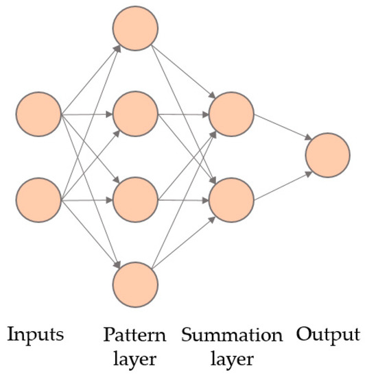
Figure 1.
Configuration of a generalized regression neural network (GRNN) with two independent numeric variables and four training cases.
Finally, the output layer has only one neuron that calculates the output by dividing the numerator and the denominator of the summation layer.
On the other hand, MLFNs consist of an input layer, one or even two hidden layers and the output layer. A MLFN is configured by specifying the number nodes in the hidden layers. The net behavior will depend on the number of nodes selected for each hidden layer, the connections weights, the bias terms that are assigned to each node, and the activation/transfer function selected to convert into output the inputs of each node. They are able to approximate complex relationships between the variables.
2.2. Lagged variable Size
One of the issues to be analyzed within this paper is the current discussion about if a larger lagged variable size allows for increasing the forecast accuracy [18] or if a shorter size is preferred based on avoiding to miss short-run predictability information [20,21]. Another issue will be whether lagged variable regression results are very sensitive regarding their size [19] or not [18].
Lagged variables are generated by a number of linear time-delayed input terms or past values, normally in ascending order, such as P(t−n)… P(t−2), P(t−1), to estimate the output value P(t) [34]. They are also referred to as rolling windows [35].
To undergo a first estimation of the number of time-delayed terms that should form the lagged variables (n), there are several alternatives that can be selected, including the one developed by Ren et al. [36], which uses the seasonal characteristic that appears in the autocorrelation function (ACF) plot, although this value is not always available.
Other common approach is to approximate the value by determining the square root of the amount of data available to undertake the analysis [26]:
Another alternative is the one used also by Matyjaszek et al. [26], in which the adequate number of time-delayed terms, k, that should form each input layer is calculated as follows:
Total nº of data ≤ n2 + 2n + 1,
n = 1 + k + 1
2.3. Adding Intrinsic Signals to the Lagged Variables
Up to date and in order to improve the forecast accuracy by adding signals to the lagged variables, research is focused on the extrinsic ones [24,25]. This paper would analyze whether it is feasible to optimize predictor variables by adding intrinsic signals, so that the neural network will have more information available; thus, a better forecast could be made. For this purpose, the order in the time series of each lagged variable would be used, so the ANN could exploit this feature.
This line of thinking is congruent with the work developed by Barabási [37], who states that there is a huge disconnect between network science and deep learning; although ANN are abstractions of natural processes, some of the key neural networks could not be more ignorant about real networks. Main deep learning algorithms treat network features, like degree, as simple variables. Thus, they cannot truly exploit the network effects, which are the essence of these systems, as in networked systems the key information is in the relationships between the connected components (i.e., in the links or edges, which are the direct interactions between nodes), not in the node attributes.
Table 1 presents an example of the first through tenth lagged variables used in a model with five time-delayed input terms: P(t−k)… P(t−2), P(t−1), with k = 5, as well as the output to be estimated: P(t).

Table 1.
First through tenth lagged variables with five time-delayed input terms, and the output to be estimated (t).
Table 2 presents the same first through tenth lagged variables with five time-delayed input terms plus the order in the time series of each lagged variable, as well as the output to be estimated: P(t).
Table 2.
First through tenth predictor variables with 5 time-delayed input terms plus the order in the time series of each lagged variable, and the output to be estimated (t).
2.4. Figures of Merit
The experimental results will be evaluated using the two most common figures of merit [38], namely, the root mean squared error (RMSE) and the mean absolute error (MAE).
The RMSE is an excellent general-purpose error measure used for numerical predictions. It amplifies and penalizes large errors and can be expressed as follows:
where At is the actual value, Ft is the forecasted value, and n is the number of forecasted values.
The MAE is used to measure how close the predictions are to the outcomes and can be expressed as follows:
Chai and Draxler [39] proposed the use of a combination of metrics including but not limited to the RMSE and the MAE. Conversely, Carta et al. [40], when addressing wind resource prediction, proposed using the MAE, the MAPE and the index of agreement (IoA).
In this paper, the standard deviation of absolute error (STD of AE) was selected to complement these measures as in Lazaridis [38], characterizing the dispersion of the absolute errors.
3. Results
3.1. Coking Coal
The dataset used was the Colombia hard coking coal monthly prices free on board (FOB) for the period from January 1991 to December 2015, as publicly disclosed by the Colombian Mining Information System [41], totaling 300 data points. The dataset is presented in Figure 2.
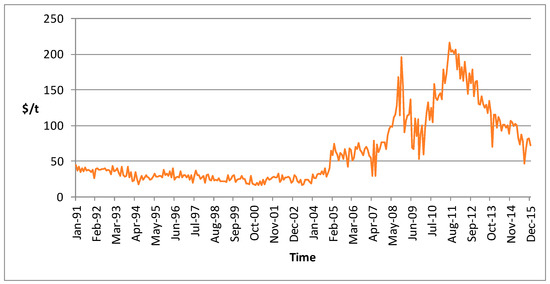
Figure 2.
Colombia hard coking coal monthly prices FOB from January 1991 to December 2015 [41].
In first place, GRNNs and MLFNs with 2–6 nodes in the first hidden layer (as the second layer is seldom needed for better prediction accuracy) were tested using the best net search function that is available in NeuralTools.
Table 3 presents the results of this best net search, where the configuration of the lagged variables was made using 19 time-delayed terms, which was the lagged variable size given by the seasonal characteristic that appears in the autocorrelation function (ACF) plot of the transformed time series when representing a consistent genome [26,42]. The results showed that the GRNN improved all the MLFN models, as stated for most cases by Modaresi et al. [43], so this will be the ANN to be used in this paper.
Table 3.
Best net search.
To undergo a first estimation of the number of time-delayed terms that should form the lagged variables, the square root of the amount of data available to undertake the analysis was calculated:
Using the other alternative previously mentioned, the value obtained is as follows:
300 ≤ n2 + n + 1 => n = 16.32,
k = n −2 = 14.32
Nevertheless, the GRNN will be trained starting with 12 time-delayed input terms and up to 24 time-delayed input terms, a range that includes the previous values of k as well as one and two complete year periods [18].
This allows considering almost any periodical aspect that may be hidden within the time-series values but without drastically reducing the sample size requirements according to Turmon and Fine [44]. The results from the GRNN training are presented in Table 4.
Table 4.
Training results for the GRNN model of the Colombian coking coal time series, from 12 to 24 time-delayed input terms (total number of data points is 300).
Based on these measures, the best result was obtained with 19 time-delayed input terms, which was the lagged variable size given by the seasonal characteristic that appears in the autocorrelation function (ACF) plot of the transformed time series when representing a consistent genome [26].
The figures of merit were root mean squared error (RMSE) of 4.550, mean absolute error (MAE) of 2.784 and standard deviation of absolute error of 3.599. With 30% tolerance, the percentage of bad predictions was 8.5409%.
Then, it was checked if it was feasible to optimize the predictor variables by adding intrinsic signals to the lagged variables so that the ANN would have more information available, and thus, a better forecast could be achieved.
For this purpose, the order of the lagged variables in the time series was considered. Using these predictor variables, results from the training of the GRNN are presented in Table 5.
Table 5.
Training results for the GRNN model of the Colombian coking coal time series, from 12 to 24 time-delayed input terms and including the order in the time series of the lagged variables (total number of data points is 300).
The best result was obtained with 24 time-delayed input terms, with a RMSE of 3.376, a MAE of 2.286 and a standard deviation of absolute error of 2.485. With 30% tolerance, the percentage of bad predictions was 2.5362%. Thus, the order in the time series of the lagged variables clearly improved the model’s forecasting performance, as it significantly reduced the RMSE, the MAE, the standard deviation of absolute error and the percentage of bad predictions.
3.2. Natural Gas
The second raw material for energy production analyzed was natural gas. The dataset used was natural gas prices in Europe for the period from January 1991 to August 2019, totaling 344 values.
Prices were obtained from the World Bank [45] and are presented in Figure 3 in MMBtu, also known as million British thermal units, with 1 MMBtu = 28.263682 m3 of natural gas at 1 °F.
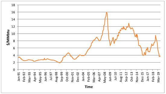
Figure 3.
Natural gas prices in Europe for the period from January 1991 to August 2019 [45].
As no seasonal characteristic appears in the autocorrelation function (ACF), in order to estimate the number of time-delayed input terms, the following calculations were made:
344 ≤ n2 + n + 1 => n = 17.54
k = n −2 = 15.54
Nevertheless, the GRNN was trained with lagged variables starting with 12 time-delayed input terms and up to 24 time-delayed input terms, using the same interval as in the coking coal case and for the same reasons.
The results from the training of the GRNN are presented in Table 6.
Table 6.
Training results for the GRNN model of the European natural gas time series, from 12 to 24 time-delayed input terms (total number of data points is 344).
The best result was obtained with 12 time-delayed input terms, with a RMSE of 0.06273, a MAE of 0.03456 and a standard deviation of absolute error of 0.05235. With 5% tolerance, the percentage of bad predictions was 4.8193%. A 5% tolerance was used this time, as with a 30% tolerance the percentages of bad predictions were always zero.
Then, the GRNN was trained using the same number of time-delayed input terms but considering the order in the time series of each lagged variable. The results from the training of the GRNN are presented in Table 7. In this case, the best result was obtained with 14 time-delayed input terms, with a RMSE of 0.01970, a MAE of 0.01032 and a standard deviation of absolute error of 0.01678. With 5% tolerance, the percentage of bad predictions decreased to zero.
Table 7.
Training results for the GRNN model of the European natural gas time series, from 12 to 24 time-delayed input terms and including the order in the time series of the lagged variables (total number of data points is 344).
Thus, again, the order in the time series of the lagged variables clearly improved the model’s forecasting performance, as it significantly reduced the RMSE, the MAE, the standard deviation of absolute error and the percentage of bad predictions.
3.3. Crude Oil
The third raw material for energy production analyzed was crude oil. The dataset used was that of Brent crude oil prices for the same period as for the natural gas: January 1991 to August 2019, totaling 344 values. Again, prices were obtained from the World Bank [45] and are presented in Figure 4 in $/bbl, that is, dollars per barrel, with 1 barrel being approximately 159 liters.
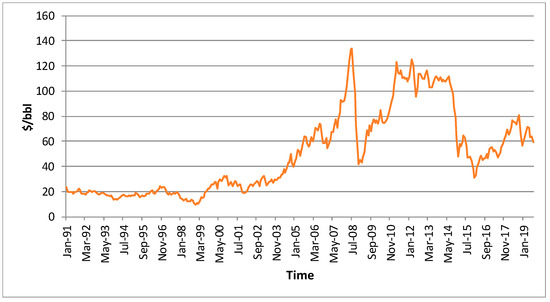
Figure 4.
Brent crude oil prices for the period from January 1991 to August 2019 [45].
The number of estimated time-delayed input terms that should be used were the same as in the case of natural gas and crude oil, as the number of data points was the same in all cases (344).
The GRNN was trained again with lagged variables starting with 12 time-delayed input terms and up to 24 time-delayed input terms. The results from the training of the GRNN are presented in Table 8.
Table 8.
Training results of the GRNN model for the Brent crude oil time series, from 12 to 24 time-delayed input terms (total number of data points is 344).
The best result was obtained with 23 time-delayed input terms, with a RMSE of 1.177, a MAE of 0.6645 and a standard deviation of absolute error of 0.971. With 5% tolerance, the percentage of bad predictions was 23.0530%.
Then, the GRNN was trained using the same number of time-delayed input terms but considering the order in the time series of each lagged variable. The results from the training of the GRNN are presented in Table 9.
Table 9.
Training results of the GRNN model for the Brent crude oil time series, from 12 to 24 time-delayed input terms including the order in the time series of the lagged variables (total number of data points is 344).
The best result was obtained with 14 time-delayed input terms, with a RMSE of 0.0281, a MAE of 0.0178 and a standard deviation of absolute error of 0.0218. With 5% tolerance, the percentage of bad predictions decreased again to zero.
With 12 time-delayed input terms, it is clear that the ANN was able to learn the exact configuration of the time series, but only in this case.
Thus, the order in the time series of the lagged variables clearly improved the model’s forecasting performance, as it significantly reduced the RMSE, the MAE, the standard deviation of absolute error and the percentage of bad predictions.
3.4. Coal
The fourth and last raw material for energy production analyzed was coal. The dataset used was that of Australian coal prices for the same period as crude oil and natural gas: January 1991 to August 2019. Prices were also obtained from the World Bank [45] and are presented in Figure 5 in $/t.
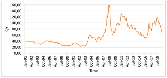
Figure 5.
Australian coal prices for the period January from 1991 to August 2019 [45].
The number of estimated time-delayed input terms that should be used were the same as in the case of natural gas and crude oil, as the number of data points was the same in all cases (344).
The GRNN was trained again with lagged variables starting with 12 time-delayed input terms and up to 24 time-delayed input terms, as in the case of European natural gas and Brent crude oil. The results from the training of the GRNN are presented in Table 10.
Table 10.
Training results of the GRNN model for the Australian coal time series, from 12 to 24 time-delayed input terms (total number of data points is 344).
The best result was obtained with 19 time-delayed input terms, with a RMSE of 1.3280, a MAE of 0.7397 and a standard deviation of absolute error of 1.1029. With 5% tolerance, the percentage of bad predictions was 15.6923%.
Then, the GRNN was trained using the same number of time-delayed input terms but considering the order in the time series of each lagged variable. The results from the training of the GRNN are presented in Table 11.
Table 11.
Training results for the GRNN models of the Australian coal time series, from 12 to 24 time-delayed input terms and including the order in the time series of the lagged variables (total number of data points is 344).
The best result was obtained with 22 time-delayed input terms, with a RMSE of 1.3678, a MAE of 0.8185 and a standard deviation of absolute error of 1.0959. With 5% tolerance, the percentage of bad predictions was 16.7702%.
In this case, adding the order in the time series of each lagged variable only improved the standard deviation of absolute error.
Nevertheless, if the RMSE and MAE were compared with the training results obtained without adding the order in the time series of each lagged variable, although slightly higher, they were very similar to the best results, and better than the rest of the training results.
Thus, the differences between both options were almost negligible.
4. Discussion and Conclusions
This paper applied a heuristic approach to optimize the predictor variables in artificial neural networks when forecasting raw material prices for energy production to achieve a better forecast.
Two goals are (1) to determine the optimum number of time-delayed terms or past values forming the lagged variables and (2) to optimize predictor variables by adding intrinsic signals to the lagged variables.
The experimental results were evaluated using the two most common figures of merit, the root mean squared error (RMSE) and the mean absolute error (MAE), as well as the standard deviation of absolute error, as the scientific literature proposes the use of a combination of metrics including RMSE and MAE, but not being limited to them.
Results demonstrated, first, that in opposition to scientific literature when addressing lagged variable size, a larger size did not allow for increasing the forecast accuracy, and that smaller sizes did not reduce the estimation accuracy. Moreover, the lagged variable regression results were very sensitive regarding their size.
In the three raw materials with the same number of cases (natural gas, crude oil and coal), the best results were obtained with rolling window sizes of 12, 23 and 19, respectively. Furthermore, it was possible to verify an important effect of the lagged variable size on the results, with differences that in some cases were larger than 20%.
Thus, and in opposition again to scientific literature indicating that there are no proper methods to select an optimum size so arbitrary selections have to be made, it is recommendable to address this question by trial and error method, although the approximate size can be estimated in order to select the complete year’s period range to which this value belongs, e.g., 12–24 months or 24–36 months. This will allow considering any periodical aspect that may be hidden within the time series values, but without drastically reducing or increasing the sample size requirements for neural networks.
Second, in three of the four raw materials analyzed (coking coal, natural gas and crude oil), it was possible to improve the forecast accuracy by adding the order in the time series of the lagged variables to form the predictor variables. The best results were achieved with rolling window sizes of 24, 14 and 14, respectively.
In the case of the Australian coal, this process only improved the standard deviation of absolute error. Nevertheless, if the RMSE and MAE were compared with the training results obtained without adding the order, although slightly higher, they were very similar to the best results and better than the rest of the training results without adding the order.
As the differences between both options were almost negligible, it is possible to recommend adding the order in the time series of each lagged variable to the predictor variable in all cases.
Third, only with the Brent crude oil with 12 time-delayed input terms and considering the order in the time series of the lagged variables, the ANN was able to learn or deduct the exact configuration of the time series. This is completely congruent with the fact that there is a huge disconnect between network science and deep learning, as the key information is in the relationships between the connected components, not in the node attributes.
Concluding, the findings presented in this paper have an immediate practical application addressing the forecast of time series by means of ANN that consider lagged variables, without being restricted to the studied case of raw material prices for energy production.
Any forecast may be optimized just by adding an intrinsic signal to the predictor variable consisting of the order in the time series of each lagged variable. By doing this way, the ANN will be able to exploit this feature, something that will not happen otherwise. In most of the cases, figures of merit may improve (may be reduced) up to a 20%, with the consequent benefit for decision-makers regarding savings, efficiency/benefit gains and/or lower risk.
Regarding the size of the lagged variable, a selection should be made about the period that will be analyzed in order to undergo a trial and error process. This selection should follow the procedure shown in this paper or other ones that may be found in the scientific literature.
Further research should address different issues such as the use of more intrinsic signals. Regarding this issue, authors have made interesting preliminary approaches by considering the transgenic time series theory that allows eliminating anomalous phenomena from the time series. Augmenting the lagged variables within this anomalous period with a ‘1’ and the rest with a ‘0’, or vice versa, it was possible to improve a priori the figures of merit.
Another area of interesting future research will be to develop a procedure to determine accurately the number of time-delayed input terms that should be used when considering the order in the time series of the lagged variables. While the seasonal characteristic that appears in the autocorrelation function (ACF) plot is valid before augmenting the lagged variables, later this figure is no longer valid, so a new approach should be addressed. Nevertheless, nothing is yet developed addressing the time series with an ACF plot that does not allow one to extract a seasonal characteristic. Again, the transgenic time series theory could be of help in these cases.
Finally, it should be addressed by future research why in the case of Australian coal, or in similar cases, it was not possible to improve the figures of merit by adding to the predictor variable the order in the time series of each lagged variable.
Author Contributions
Conceptualization, M.M. and P.R.F.; methodology, A.K. and P.R.F.; software, G.F.V.; validation, K.W.; formal analysis, G.F.V.; investigation, A.K., P.R.F. and M.M.; resources, G.F.V.; data curation, G.F.V.; writing—original draft preparation, M.M. and P.R.F.; writing—review and editing, A.K.; visualization, P.R.F.; supervision, K.W. and A.K.; and project administration, P.R.F. and K.W. All authors have read and agree to the published version of the manuscript.
Funding
This research received no external funding.
Acknowledgments
The doctoral research fellowship from the Technological Research Foundation “Luis Fernández Velasco” in Mineral and Mining Economics at the School of Mining, Energy and Material Engineering from the University of Oviedo (Spain) for the first author is highly appreciated.
Conflicts of Interest
The authors declare no conflict of interest.
References
- Bermejo, J.F.; Fernández, J.F.G.; Polo, F.O.; Márquez, A.C. A review of the use of artificial neural network models for energy and reliability prediction. A study of the solar PV, hydraulic and wind energy sources. Appl. Sci. 2019, 9, 1844. [Google Scholar] [CrossRef]
- Ali, S.M.; Paul, S.K.; Azeem, A.; Ahsan, K. Forecasting of optimum raw material inventory level using artificial neural network. Int. J. Oper. Quant. Manag. 2011, 17, 333–348. [Google Scholar]
- Gabralla, L.; Abraham, A. Computational modeling of crude oil price forecasting: a review of two decades of research. Int. J. Comput. Inf. Syst. Ind. Manag. Appl. 2013, 5, 729–740. [Google Scholar]
- Hyup Roh, T. Forecasting the volatility of stock price index. Expert Syst. Appl. 2007, 33, 916–922. [Google Scholar] [CrossRef]
- Panapakidis, I.P.; Dagoumas, A.S. Day-ahead electricity price forecasting via the application of artificial neural network based models. Appl. Energy 2016, 172, 132–151. [Google Scholar] [CrossRef]
- Hadavandi, E.; Shavandi, H.; Ghanbari, A. Integration of genetic fuzzy systems and artificial neural networks for stock price forecasting. Knowledge-Based Syst. 2010, 23, 800–808. [Google Scholar] [CrossRef]
- Mombeini, H.; Yazdani-chamzini, A. Modeling Gold Price via Artificial Neural Network. J. Econ. Bus. Manag. 2015, 3, 3–7. [Google Scholar] [CrossRef]
- Sánchez Lasheras, F.; de Cos Juez, F.J.; Suárez Sánchez, A.; Krzemień, A.; Riesgo Fernández, P. Forecasting the COMEX copper spot price by means of neural networks and ARIMA models. Resour. Policy 2015, 45, 37–43. [Google Scholar] [CrossRef]
- Colla, V.; Matino, I.; Dettori, S.; Cateni, S.; Matino, R. Reservoir Computing Approaches Applied to Energy Management in Industry. In Engineering Applications of Neural Networks, Proceedings of the 20th International Conference EANN, Xersonisos, Crete, Greece, 24–26 May 2019; Macintyre, J., Iliadis, L., Maglogiannis, I., Jayne, C., Eds.; Springer: Cham, Switzerland, 2019; pp. 66–79. [Google Scholar]
- Baffour, A.A.; Feng, J.C.; Taylorb, E.K. A hybrid artificial neural network-GJR modeling approach to forecasting currency exchange rate volatility. Neurocomputing 2019, 365, 285–301. [Google Scholar] [CrossRef]
- Sánchez Lasheras, F.; Vilán Vilán, J.A.; García Nieto, P.J.; del Coz Díaz, J.J. The use of design of experiments to improve a neural network model in order to predict the thickness of the chromium layer in a hard chromium plating process. Math. Comput. Model. 2010, 52, 1169–1176. [Google Scholar] [CrossRef]
- Bo, L.; Cheng, C. First-Order Sensitivity Analysis for Hidden Neuron Selection in Layer-Wise Training of Networks. Neural Process. Lett. 2018, 48, 1105–1121. [Google Scholar]
- Pontes, F.J.; Amorim, G.F.; Balestrassi, P.P.; Paiva, A.P.; Ferreira, J.R. Design of experiments and focused grid search for neural network parameter optimization. Neurocomputing 2016, 186, 22–34. [Google Scholar] [CrossRef]
- Li, F.; Zurada, J.M.; Liu, Y.; Wu, W. Input Layer Regularization of Multilayer Feedforward Neural Networks. IEEE Access 2017, 5, 10979–10985. [Google Scholar] [CrossRef]
- Li, F.; Zurada, J.M.; Wu, W. Smooth group L1/2 regularization for input layer of feedforward neural networks. Neurocomputing 2018, 314, 109–119. [Google Scholar] [CrossRef]
- Xu, X. Price dynamics in corn cash and futures markets: cointegration, causality, and forecasting through a rolling window approach. Financ. Mark. Portf. Manag. 2019, 33, 155–181. [Google Scholar] [CrossRef]
- Velázquez Medina, S.; Carta, J.A.; Portero Ajenjo, U. Performance sensitivity of a wind farm power curve model to different signals of the input layer of ANNs: Case studies in the Canary Islands. Complexity 2019, 2019, 2869149. [Google Scholar]
- Liu, G.D.; Su, C.W. The dynamic causality between gold and silver prices in China market: A rolling window bootstrap approach. Financ. Res. Lett. 2019, 28, 101–106. [Google Scholar] [CrossRef]
- Tang, C.F.; Abosedra, S. Tourism and growth in Lebanon: new evidence from bootstrap simulation and rolling causality approaches. Empir. Econ. 2016, 50, 679–696. [Google Scholar] [CrossRef]
- Timmermann, A. Elusive return predictability. Int. J. Forecast. 2008, 24, 1–18. [Google Scholar] [CrossRef]
- Tang, C.F.; Chua, S.Y. The savings-growth nexus for the Malaysian economy: A view through rolling sub-samples. Appl. Econ. 2012, 44, 4173–4185. [Google Scholar] [CrossRef]
- Frank, E.; Hall, M.A.; Witten, I.H. The WEKA Workbench. Online Appendix for "Data Mining: Practical Machine Learning Tools and Techniques", 4th ed.; Morgan Kaufmann: Cambridge, MA, USA, 2016. [Google Scholar]
- Hall, M.; Frank, E.; Holmes, G.; Pfahringer, B.; Reutemann, P.; Witten, I.H. The WEKA Data Mining Software: An Update. ACM SIGKDD Explor. Newsl. 2009, 11(1), 10–18. [Google Scholar] [CrossRef]
- Tavakoli, S.; Mousavi, A.; Komashie, A. Flexible data input layer architecture (FDILA) for quick-response decision making tools in volatile manufacturing systems. IEEE Int. Conf. Commun. 2008, 1, 5515–5520. [Google Scholar]
- Uykan, Z.; Koivo, H.N. Analysis of Augmented-Input-Layer RBFNN. IEEE Trans. Neural Netw. 2005, 16, 364–369. [Google Scholar] [CrossRef]
- Matyjaszek, M.; Riesgo Fernández, P.; Krzemień, A.; Wodarski, K.; Fidalgo Valverde, G. Forecasting coking coal prices by means of ARIMA models and neural networks, considering the transgenic time series theory. Resour. Policy 2019, 61, 283–292. [Google Scholar] [CrossRef]
- Hyndman, R.; Khandakar, Y. Automatic time series forecasting: The forecast package for R. J. Stat. Softw. 2008, 27, 1–22. [Google Scholar] [CrossRef]
- Ong, C.S.; Huang, J.J.; Tzeng, G.H. Model identification of ARIMA family using genetic algorithms. Appl. Math. Comput. 2005, 164, 885–912. [Google Scholar] [CrossRef]
- Specht, D.F. A general regression neural network. IEEE Trans. Neural Netw. 1991, 2, 568–576. [Google Scholar] [CrossRef]
- Krzemień, A.; Riesgo Fernández, P.; Suárez Sánchez, A.; Sánchez Lasheras, F. Forecasting European thermal coal spot prices. J. Sustain. Min. 2015, 14, 203–210. [Google Scholar] [CrossRef]
- Krzemień, A. Dinamic fire risk prevention strategy in underground coal gasification processes by means of artificial neural networks. Arch. Min. Sci. 2019, 64, 3–19. [Google Scholar]
- García Nieto, P.J.; Sánchez Lasheras, F.; García-Gonzalo, E.; de Cos Juez, F.J. PM10 concentration forecasting in the metropolitan area of Oviedo (Northern Spain) using models based on SVM, MLP, VARMA and ARIMA: A case study. Sci. Total Environ. 2018, 621, 753–761. [Google Scholar] [CrossRef]
- Panella, M.; Barcellona, F.; D’Ecclesia, R.L. Forecasting Energy Commodity Prices Using Neural Networks. Adv. Decis. Sci. 2012, 2012, 1–26. [Google Scholar] [CrossRef]
- Li, Z.; Best, M. Optimization of the Input Layer Structure for Feed-Forward Narx Neural Networks. Int. J. Electr. Comput. Energ. Electron. Commun. Eng. 2015, 9, 673–678. [Google Scholar]
- Morantz, B.H.; Whalen, T.; Zhang, G.P. A weighted window approach to neural network time series forecasting. In Neural Networks in Business Forecasting; Zhang, G.P., Ed.; IRM Press: Hershey, PA, USA, 2004. [Google Scholar]
- Ren, Y.; Suganthan, P.N.; Srikanth, N.; Amaratunga, G. Random vector functional link network for short-term electricity load demand forecasting. Inf. Sci. 2016, 367, 1078–1093. [Google Scholar] [CrossRef]
- Barabási, A.-L. Network Science, 1st ed.; Cambridge University Press: Cambridge, UK, 2016. [Google Scholar]
- Lazaridis, A.-G. Prosody Modelling using Machine Learning Techniques for Neutral and Emotional Speech Synthesis. Ph.D. Thesis, University of Patras, Patras, Greece, 2011. [Google Scholar]
- Chai, T.; Draxler, R.R. Root mean square error (RMSE) or mean absolute error (MAE)? -Arguments against avoiding RMSE in the literature. Geosci. Model Dev. 2014, 7, 1247–1250. [Google Scholar] [CrossRef]
- Carta, J.A.; Cabrera, P.; Matías, J.M.; Castellano, F. Comparison of feature selection methods using ANNs in MCP-wind speed methods. A case study. Appl. Energy 2015, 158, 490–507. [Google Scholar] [CrossRef]
- System of Colombian Mining Information. Available online: http://www1.upme.gov.co/simco/Paginas/default.aspx (accessed on 11 May 2017).
- Riesgo García, M.V.; Krzemień, A.; Manzanedo del Campo, M.Á.; Escanciano García-Miranda, C.; Sánchez Lasheras, F. Rare earth elements price forecasting by means of transgenic time series developed with ARIMA models. Resour. Policy 2018, 59, 95–102. [Google Scholar] [CrossRef]
- Modaresi, F.; Araghinejad, S.; Ebrahimi, K. A Comparative Assessment of Artificial Neural Network, Generalized Regression Neural Network, Least-Square Support Vector Regression, and K-Nearest Neighbor Regression for Monthly Streamflow Forecasting in Linear and Nonlinear Conditions. Water Resour. Manag. 2018, 32, 243–258. [Google Scholar] [CrossRef]
- Turmon, M.J.; Fine, T.L. Sample Size Requirements for Feedforward Neural Networks. In Proceedings of the Advances in Neural Information Processing Systems 7, Denver, CO, USA, 28 November 28–1 December 1994; pp. 1–18. [Google Scholar]
- The World Bank. Available online: http://pubdocs.worldbank.org/en/561011486076393416/CMO-Historical-Data-Monthly.xlsx (accessed on 24 September 2019).


© 2020 by the authors. Licensee MDPI, Basel, Switzerland. This article is an open access article distributed under the terms and conditions of the Creative Commons Attribution (CC BY) license (http://creativecommons.org/licenses/by/4.0/).