Abstract
The buzz phenomenon of a typical supersonic inlet is analyzed on the basis of numerical simulations and duct acoustic theory. Considering that the choked inlet could be treated as a duct with one end closed, a one-dimensional (1D) mathematical model based on the duct acoustic theory is proposed to describe the periodic pressure oscillation of the little buzz and the big buzz. The results of the acoustic model agree well with that of the numerical simulations and the experimental data. It could verify that the dominated oscillation patterns of the little buzz and the big buzz are closely related to the first and second resonant mode of the standing wave, respectively. The discrepancies between the numerical simulation and the ideal acoustic model might be attributed to the viscous damping in the fluid oscillation system. In order to explore the damping, a small perturbation jet is introduced to trigger the resonance of the buzz system and the nonlinear amplification effect of resonance might be helpful to estimate the damping. Through the comparison between the linear acoustic model and the nonlinear simulation, the calculated pressure oscillation damping of the little buzz and the big buzz are 0.33 and 0.16, which could be regarded as an estimation of real damping.
1. Introduction
Inlet buzz is a severely unstable flow oscillation phenomenon observed in supersonic and hypersonic air-breathing systems [1]. When buzz occurs, the shock system moves violently and periodically along the inlet compression surface and the internal flow duct of the inlet suffers dramatic pressure oscillations. As a result of the inlet buzz, the established air capture and compression system could be destroyed, which leads to oscillatory mass feeding the burner, unstable distribution of force loads, structural vibration, and even flight mission failure. [2,3].
Inlet buzz was first observed by Oswatitsch [4] in an experimental exploration of the aerodynamic performance of an asymmetrically configured missile inlet system flying at high supersonic speed. With efforts devoted to studying this phenomenon experimentally and numerically for decades, a general understanding categorizes buzz into two types, namely, little buzz and big buzz. Two prevailing triggering mechanisms were proposed to find the origin of inlet buzz. In the little buzz phase, the Ferri criterion [5] suggested that the instability is characterized by the vortex sheet resulting from the intersection of oblique shocks and terminal shock. The vortex sheet impinges with the cowl inner surface, causing flow separation and blockage of the entrance. In contrast, Dailey criterion [6] deemed that strong shock-induced separation on the compression surface chokes the flow and finally ignites big buzz.
Subsequent studies followed their propositions and more attention was given to the frequencies of little buzz and big buzz. In the experiment of Fisher et al. [7], the two forms of oscillations termed little buzz and big buzz were observed successively with the reduction of the inlet mass flow rate. They identified little buzz and big buzz by amplitude and claimed that the frequencies of them are similar, while it is not true in the other studies. Nagashima et al. [8] carried out an inlet buzz experiment by controlling the throttling ratio (T.R.) and observed the little buzz with a characteristic frequency of about 120 Hz and the big buzz of 360 Hz. The amplitude of the pressure oscillation in the inlet duct did not change significantly. Trapier et al. [9,10], based on a mixed compression rectangular inlet, detected the phenomenon of little buzz with high frequency and low amplitude, and big buzz with low frequency and high amplitude. Lee et al. [11] investigated two type of small-sized supersonic inlet models: rectangular and axisymmetric inlets. The based frequency of big buzz for both models are similar, while that of little buzz are affected by the disturbance generated from the separation. Soltani et al. [12] observed a new pattern of buzz with large amplitude and large frequency, which has features of both little buzz and big buzz. Both amplitude and frequency of buzz oscillations vary with the downstream backpressure. As the freestream Mach number is increased, the dominant frequency of buzz flow is decreased. Tan et al. [13,14,15] referred to the phase between little buzz and big buzz as mixed buzz (or medium buzz). These three buzz phenomena probably share a common origin. Despite different frequencies of little buzz and big buzz under different experimental conditions, the oscillation behavior of supersonic inlet buzz is considered to be linked with an acoustic feedback mechanism [16,17].
To unfold the oscillatory mechanism of the inlet buzz phenomenon, Dailey [6] experimented with a supersonic inlet and an organ pipe, noting that there is a link between the oscillatory frequencies and the acoustic resonance modes. In Nagashima et al.’s experimental work [8], the frequency features of both little buzz and big buzz also suggested the link between inlet buzz and acoustic resonance. Hankey and Shang [18] considered the inlet buzz as a self-excited oscillation phenomenon and formulated a relationship for self-excited oscillation frequency. It is found that the fundamental frequency of acoustic resonance obtained by this formula coincided with a number of inlet buzz flows they collected. The first numerical computations of inlet buzz with Navier–Stokes equations were conducted by Newsome [16] on an external compression axisymmetric inlet [8] and the frequency obtained from numerical simulation agreed with the fundamental acoustic frequency derived from a formula proposed by him. Considering the discrepancy between real inlet duct and the ideal acoustic duct, through numerical simulations using the Dailey’s inlet geometry [6], Lu and Jain [17] revised the upstream feedback mechanism which attributed the buzz cycle to the coupling of the acoustic resonance occurred inside the plenum chamber and the instability around the inlet entrance. Chima [19] and Hong [20] substantiate the relation between inlet buzz and duct acoustic resonance. Recent progress by Tan et al. [14] revealed two acoustic feedback loops are simultaneously established during buzz. Transition of buzz flow is attributed to the change of dominant role between two feedback loops.
Acoustic interpretation achieves good agreement in the frequency domain in various studies. However, merely focusing on the frequencies of experimental measurements and acoustic resonance modes is not enough to fully characterize this acoustical connection. A lack of understanding towards the amplitude features is not conducive to carry out an in-depth quantitative analysis on the intensity of oscillation in the fluid system and other oscillation-related parameters, such as damping. Analogous to the mechanical system, the oscillations in fluid flow could be affected by damping, particularly the acoustic wave propagating in the duct. Until now, few studies have been undertaken in the field of exploring the damping in the inlet buzz system. Nowadays, mathematic modeling has attracted the attention of researchers as a new way to describe the buzz behaviors. Chang et al. [21] introduced the deterministic learning theory and rapid recognition methods to model the oscillatory behavior and detect the buzz pattern, respectively. In their other paper [22], the idea of Moore-Greitzed model was employed to build the reduced-order model for buzz oscillations. Recently, Yamamoto et al. [23] proposed a model for the prediction of the buzz onset, which indicates that the buzz system could be represented by a delay differential equation containing a delayed negative feedback.
Based on the above understanding, the goal of this work is to establish a mathematical model involving the oscillation amplitude and explore the damping in the inlet buzz dynamic process. In this study, numerical simulation of supersonic inlet buzz was performed based on the inlet model reproduced from Nagashima et al.’s experiments [8]. Section 2 will give a description of the numerical procedure adopted in the current study, including the simulation model, grid and calculation method. Section 3 presents numerical simulation results of the frequency characteristics and the pressure oscillation characteristics of both the little buzz and the big buzz. Section 4 presents mathematical modeling of the dynamic process for acoustic resonance inside an ideal duct using acoustic theory. In our opinion, the discrepancies between the established acoustic model and the numerical simulations are mainly attributed to the influence of the viscous damping in fluid flows. In Section 5, the resonance method is adopted in the exploration of damping. Finally, Section 6 summarizes this paper.
2. Numerical Simulation Procedure
2.1. Inlet Model Configuration
As shown in Figure 1, the model is an axisymmetric supersonic inlet the same as Nagashima et al.’s experiments [8]. The inlet compresses incoming air through a conical shock generated by the cone center body and a normal shock generated by backpressure from ramjet burner or turbo engine standing at inlet cowl. Internal flow deceleration is conducted through a divergent duct until the exit airflow reaches a low subsonic speed meeting the requirements of the downstream component. At the rear of the inlet is a plug used for the exit area control. By moving the plug, the backpressure variation from the inlet downstream component could be simulated. According to Equation (1), the throttling ratio (T.R.) is defined as the area ratio of the exit to the minimum throat and the evolution from the little buzz to the big buzz would take place with the decrease of the throttling ratio. The total length L from the cowl’s leading edge to the exit of the plenum chamber is 0.635 m. The diameter D measuring at the inner surface of the cowl wall is 0.04 m. Plug axial movement controls the throttling ratio by adjusting of AE. Similar to Nagashima et al.’s work [8], four points on the center body and cowl wall are selected to obtain pressure record during the development of the inlet buzz, as shown in Figure 1. On the center body, the axial positions of P2 and P3 are 0.044 L and 0.071 L, while the axial positions of P4 and P7 on the internal cowl surface are 0.209 L and 0.986 L, respectively.
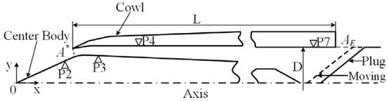
Figure 1.
Schematic diagram of the inlet model.
2.2. Computational Dynamic Mesh and Boundary Conditions
As shown in Figure 2, the two-dimensional dynamic mesh composed of quadrilateral cells was employed for the numerical simulation of the buzz phenomenon and the computational domain is divided into three parts, Fluid 1, Fluid 2, and Fluid 3. Fluid 1 and Fluid 2 are both fixed while the area of Fluid 3 is changed with the movement of the plug. The dynamic mesh method of Layering with an option of Height Based is selected. The zone type of Fluid 3 is a rigid body and the four boundaries surrounding this domain are interface 2, axis GH, inner wall LM, and plug wall GN, whose types are stationary, deforming, deforming, and rigid body, respectively. The boundary of the plug wall moves forward with a speed of 32.5 mm/s [20]. In a decreasing throttling ratio process, the first layer cells on the plug wall merge with the next layer when the cell height is below to a threshold controlled by the collapse factor (0.5) and a reference of cell height (0.0001 mm). The computational domain of the above three parts contains 21 blocks in total, of which Fluid 3 consists of three blocks. Data passing between Fluid 2 (or Fluid 1) and Fluid 3 is achieved through the interface 1 (or interface 2). Figure 2c–e shows the decrease of interface 1 when plug cone moves forward. To accurately resolve the boundary layer, the grid cells near the solid wall are denser. The non-dimensional height of the first layer cells on the wall is guaranteed for y+ < 10. Starting from the first-layer grid points, a constant stretching ratio of 1.2 is used in the boundary layer meshing.
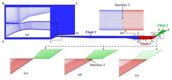
Figure 2.
Computational domain and dynamic mesh detail: (a) entrance; (b) interface 2; (c–e) interface 1.
In Figure 2, “pressure-far-field” boundary condition is imposed on sides AB and BC with constant static pressure (38,849.4 pa), static temperature (273 K), and Mach number (Mach 2), the “pressure-outlet” boundary condition is given to sides CD and EF allowing for ambient static pressure setting. Besides, sides AI and GH are both “axis” and the “wall” boundary condition is applied at the rest of the sides.
2.3. Calculation Method and Verification
The unsteady Reynolds-averaged Navier–Stokes (URANS) axisymmetric simulations were based on the steady result before buzz (T.R. = 2.48). Roe’s method [24] in combination with the monotonic upwind scheme for conservation laws (MUSCL) interpolation [25] was adopted to solve the flow equations. The turbulent flow was modeled by the Spalart–Allmaras (SA) model [26], of which the governing equations were discretized by a second-order upwind scheme. A dual-time implicit stepping method coupled with the lower-upper symmetric Gauss–Seidel scheme [27] for inner-iterations was used to simulate an unsteady flow. In addition, a no-slip adiabatic boundary condition was imposed on the solid walls. To solve the flow field accurately and efficiently, the grid refinement and the time-step sensitivity tests were carried out in advance. For more detail of verification of the adopted numerical method please refer to [28].
3. Analysis of Numerical Results
3.1. Frequency Characteristics
In the experiment of Nagashima [8], it was observed that a low-frequency oscillation pattern was changed to a high-frequency pattern as the throttling ratio (T.R.) decreased, while oscillation amplitude did not change significantly. In present study, the criterion for identifying the little buzz and big buzz is their frequency characteristics.
Figure 3 shows the typical frequency characteristics of two types of buzz phenomenon and their evolution. The Stockwell transform (S-transform) was adopted in time-frequency analysis on the pressure signal of P2 to obtain different frequencies existing in the buzz development. Several successive phases are visible in the time history of the pressure. Before buzz, there are no pressure fluctuations. During the buzz onset, the spectrogram shows a horizontal stripe for a frequency of around 120 Hz. As the flow progressively develops into a stable little buzz, the stripe of 120 Hz shows a much higher level of amplitude and the stripe of around 360 Hz corresponding to the big buzz starting to appear. After the transition, the amplitude magnitude of big buzz frequency dominates the spectrogram and the stripe for the frequency of 120 Hz gradually disappears, meanwhile, some higher-frequency components start to become apparent. It could be inferred from the time-frequency analysis that the little buzz state contains the oscillation pattern of the big buzz, while some higher-frequency flow patterns may exist in the state of the big buzz.
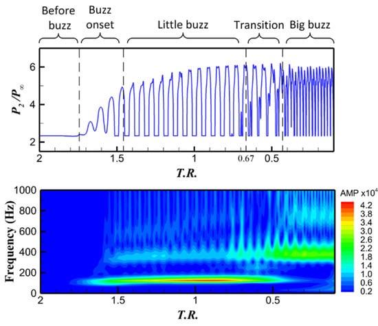
Figure 3.
Time-frequency analysis on the pressure record of P2.
3.2. Pressure Oscillation Characteristics
The unsteady properties of the static pressure fluctuations along the internal flow passage were further analyzed on the basis of the numerical simulation results. Figure 4 and Figure 5 display the pressure oscillation characteristics of the little buzz and the big buzz during a cycle period, respectively. T1 and T2 represent the cycle periods of the little buzz and the big buzz. At each moment within one cycle period, the upper half shows the static pressure contour of the entire flow field, and the lower half exhibits the static pressure curves along the internal flow passage, in which the solid and dashed curve indicate the transient and the time-averaged static pressure, respectively. In addition, pressure nodes and antinodes seem to exist in both the little buzz pattern and the big buzz pattern, as shown in Figure 4 and Figure 5.
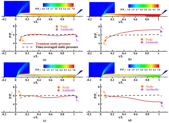
Figure 4.
Pressure oscillation characteristics of little buzz at different time periods: (a) t = 0·T1 and t = T1; (b) t = 0.25·T1; (c) t = 0.5·T1; (d) t = 0.75·T1.
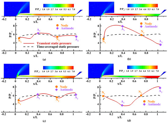
Figure 5.
Pressure oscillation characteristics of big buzz at different time periods: (a) t = 0·T2 and t = T2; (b) t = 0.25·T2; (c) t = 0.5·T2; (d) t = 0.75·T2.
The case of the little buzz is discussed firstly in Figure 4. At t = 0, the transient pressure distribution along the internal flow path is closed to the time-averaged static pressure distribution. As the air propagates downstream, the downstream pressure gradually increases. The pressure along the internal flow path shows a monotonous increase and reaches the maximum value at antinode A1, as shown in Figure 4b at t = 0.25·T1. Due to the choked exit, the downstream high-pressure air propagates upstream, and the pressure in the internal passage gradually decreases. At t = 0.5·T1, the pressure decreases to near the time-average pressure. At t = 0.75·T1, the pressure along the channel shows a monotonically decreasing trend and the static pressure at antinode A1 reaches the minimum value; At t = T1, the flow field is as same as the initial one at t = 0·T1. A little buzz period is completed and the oscillation then turns to the next period.
With regard to the big buzz in Figure 5, the oscillation pattern is different. At t = 0, the transient pressure distribution is closed to the time-averaged static pressure distribution. Hereafter, due to the exit blockage, the downstream high-pressure air in the plenum chamber propagates upstream. Consequently, the static pressure of upstream air gradually increases, and the static pressure of downstream air continually decreases. Meanwhile, the static pressure at antinode A1 oscillates from the mean value to the maximum value, and the pressure at antinode A2 fluctuates from the average value to the minimum value, as displayed in Figure 5b at t = 0.25·T2. With the reduction of the plenum chamber pressure, the upstream high pressure drives the air downstream. Accordingly, the upstream pressure continually decreases, and the downstream pressure progressively increases, as presented in Figure 5c at t = 0.5·T2 and Figure 5d t = 0.75·T2. At t = 0.75·T2, the static pressure at antinode A1 reaches the minimum value and at antinode A2 reaches the maximum value. At t = T2, the flow field is as same as the initial one, and a big buzz period is completed.
It can be seen that along the internal flow path, the pressure oscillation characteristics of the little buzz are extremely similar to a 1/4 wavelength standing wave, while that of the big buzz are closed to a 3/4 wavelength standing wave.
4. Acoustic Modeling and Error Analysis
Previous research [6,8] suggested a link between inlet buzz and acoustic resonance, and illustrated this connection in the frequency domain. Subsequent results [16,17,18] partially testified this conjecture by providing the match of characteristic frequencies of inlet buzz with theoretical predictions. However, until now, a lack of coverage on the dynamic process in amplitude aspects makes the analogy of inlet buzz with acoustic resonance still incomplete. The following part will try to establish a map covering the acoustic wave oscillatory process in frequency and amplitude aspects mathematically.
4.1. Acoustic Modeling
When buzz occurs, the downstream exit of the inlet behaves as a closed end. As a result of flow choking [16,17,18], the inlet can be approximately regarded as a duct with an open end and a closed end. As the wavelength is far outweighing the inner diameter of the duct, acoustic waves propagate in the form of plane waves inside the duct. Ideally, for a constant cross-section duct with an open end and a rigid closed end, an incoming acoustic wave spreads from the open end to the closed end at the speed of sound, and then it is reflected (known as a reflected wave). Both the incoming and the reflected waves can be mathematically described by solving the one-dimensional wave equation:
where sound pressure p′ is a function of time t and abscissa x. Mathematically, the sound pressure in the form of p′ (t/T − x/λ) and p′ (t/T + x/λ) would satisfy the one-dimensional wave equation. Considering that the geometry of the inlet has been simplified as a constant cross-section duct, ideally, the cosine function is selected as the approximate waveform of the incoming wave. Therefore, an incoming wave with a period of T, a wavelength of λ, and sound pressure amplitude of could be written as follows:
The incoming wave is completely reflected at the closed end of the duct. There is no energy loss in this process, however, the phase of the newly formed wave is changed by π. Therefore, in the presence of Equations (2) and (3), the sound pressure of a reflected wave could be written as
During the propagation of acoustic waves in the duct, a standing wave is formed by the superposition of incoming and reflected waves. The sound pressure at any position on the standing wave is the sum of the sound pressure of incoming wave and reflected wave, namely
It can be perceived from Equation (5) that the sound pressure at any place on the standing wave oscillates with the same period, and the amplitudes at different locations can be predicted by
According to Equation (6), the amplitude at certain locations on the standing wave is always zero, while the amplitude is maximum at some positions. The former positions are called nodes, and the latter positions are antinodes [17,18]. Furthermore, the exact locations of nodes and antinodes can be easily calculated according to Equation (6). The positions of the nodes are expressed as
and the locations of the antinodes are
4.1.1. Frequency Behaviors
The length of the duct (L) is identical to the total length (L) of the inlet defined in Figure 1. According to the acoustic theory applied in a duct, when the wavelength (λ) of the propagating acoustic wave and the duct length (L) satisfy a relation as described in Equation (9), duct resonance will appear. The fundamental acoustic resonance frequency and higher frequency modes can be estimated by Equation (10) [16].
where c represents the speed of sound, Ma is the average Mach number of the flow, n = 1, 2, 3, etc. correspond to the first, second, third, etc. acoustic resonance frequencies, respectively. The results of numerical simulation show that c is about 327.1 m/s, and Ma is approximately 0.132. Substituting the values of c, Ma, and L into Equation (10), the calculated frequencies of the first mode and the second mode are 126 and 380 Hz, respectively. They are closed to the Nagashima et al.’s experiment (120 and 360 Hz) [8]. Consequently, it could be assumed that the dominant frequency of the inlet buzz is obtained by the acoustic resonance inside the duct.
4.1.2. Fluctuation Characteristic of Standing Wave
In order to compare the pressure oscillation characteristics of the inlet buzz, Figure 6 and Figure 7 show the standing wave resulting from the superposition of the coming wave and the reflected wave at the typical times within one period in the duct.

Figure 6.
Standing wave of first resonance mode in the duct at different time periods.
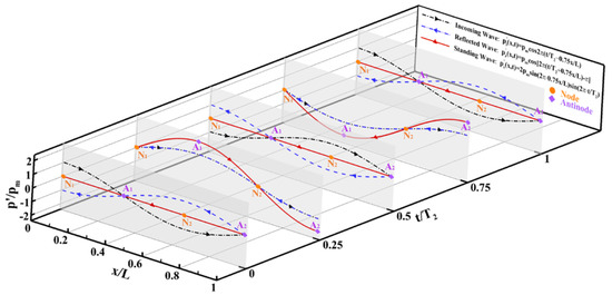
Figure 7.
Standing wave of second resonance mode in the duct at different time periods.
According to Equation (9), when n = 1, the relation between L and λ1 should be L= 0.25·λ1. Replacing λ in Equation (5) with λ1 = 4·L and T with T1 gives the equation for the first resonance mode:
According to Equation (7), the positions of the node N1 should be x = 0. Besides, using Equation (8), the locations of the antinode A1 is x = L. That is, a node and an antinode are generated at the open end and the closed end of the duct, respectively.
As shown in Figure 6, at t = 0, the sound pressure of the incoming wave and of the reflected wave at the node N1 are the maximum and the minimum, respectively. As a result, their mutual superposition is zero. At t = 0.25·T1, the incoming wave coincides with the reflected wave. The amplitude of the standing wave’s sound pressure reaches its maximum value at antinode A1. Subsequently, as the incoming and the reflected waves propagate along with contrary directions, the sound pressure at antinode A1 decreases gradually and reaches zero at t = 0.5·T1. The incoming and the reflected waves again coincide at t = 0.75·T1, and the sound pressure at antinodes A1 reaches the minimum value. After that, the pressure at antinode A1 gradually increases. At t = T1, the sound pressure at any location inside the duct is as same as the initial time. Then, the next oscillation cycle begins.
Similarly, according to Equation (9), when n = 2, the relation between L and λ2 should be L= 0.75·λ2. Replacing λ in Equation (5) with λ2 = 4/3L and T with T2 gives the equation for the second resonance mode:
According to Equation (7), the positions of the nodes N1 and N2 should be x = 0 and x = 2/3 L. Besides, using Equation (10), the locations of the antinodes A1 and A2 are x = 1/3 L and x = L.
As shown in Figure 7, at t = 0, the magnitudes of the sound pressure of the incoming wave at the nodes N1 and N2 are the maximum and the minimum, respectively, which is opposite to the pressure distribution of the reflected wave. As a result, the sound pressure of the standing wave is zero after their mutual superposition. At t = 0.25·T2, the incoming wave coincides with the reflected wave. The amplitude of the standing wave’s sound pressure reaches its maximum value at antinodes A1 and A2, corresponding to the peak and valley positions, respectively. Subsequently, as the incoming and the reflected waves propagate along with contrary directions, the sound pressure at antinode A1 decreases gradually and the sound pressure at antinode A2 increases progressively. They both reach zero at t = 0.5·T2. The incoming and the reflected waves again coincide at t = 0.75·T2, and the sound pressures at antinodes A1 and A2 reach the minimum and maximum values, respectively. After that, the pressure at antinode A1 gradually increases and the pressure at antinode A2 progressively decreases. At t = T2, the sound pressure at any location inside the duct is as same as the initial time. Then, the next oscillation cycle begins.
4.2. Error Analysis
In order to further discuss the characteristics of the inlet buzz and acoustic resonance in the duct, the standard deviation σ is introduced to evaluate the degree of pressure fluctuations, which can be calculated by
The magnitude of the standard deviation reflects the pressure oscillation severity. The larger the standard deviation, the greater the amplitude of pressure oscillations. Figure 8 presents the comparison of the standard deviation of pressure in the inlet buzz and the duct resonance. In Equation (13), the number of numerical simulation samples N is given to 6000 time-steps (about seven little buzz periods) and 2500 time-steps (about nine big buzz periods), respectively. Since the origin of the coordinate axis is at the top of the center body in the adopted numerical simulation, which is ΔL distance away from the open end of the inlet in the x-axis direction, the standard deviation curve of duct resonance was translated ΔL distance along the positive x-axis to facilitate the comparison. As shown in Figure 8, the valleys and peaks on these curves correspond to the locations of the nodes and antinodes. No matter the comparison between little buzz and first resonance mode or between big buzz and second resonance mode, the overall trends of the two cases are basically consistent.
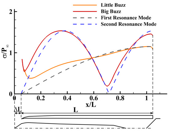
Figure 8.
Standard deviation curve of static pressure in inlet buzz and duct resonance.
The above analysis indicates that the supersonic inlet buzz phenomenon studied in this paper conform to the standing wave fluctuation in general. However, a relatively large error still exists in the range of 0.1·L to 0.4·L. Some measurements should be taken to modify the acoustic model. It is noticed that the little buzz state contains the oscillation pattern of the big buzz, while some higher-frequency flow patterns may exist in the big buzz state. Considering this fact, the error between the numerical simulation and the acoustic model may be reduced by superposing a higher-frequency and low-amplitude standing wave component . According to the result of the S-transform shown in Figure 3, the frequencies corresponding to the top two amplitudes are about 120 and 360 Hz during the little buzz, while 360 and 720 Hz during the big buzz. Therefore, the frequencies of the superposed standing wave are determined as 360 and 720 Hz to improve the first resonance mode and the second resonance mode, respectively. The modified acoustic model should take the form as follows:
Throttle ratios before and after the transition are used to obtain the amplitudes of different frequency components. The amplitudes of 120 and 360 Hz are 3.298 × 10⁴ and 1.383 × 10⁴ at T.R. = 0.7, while the amplitude of 360 and 720 Hz are 2.284 × 10⁴ and 0.818 × 10⁴ at T.R. = 0.4. Therefore, the amplitude ratios should be and . Thus Equations (14) and (15) could be rewritten as:
Figure 9 shows the comparison between the inlet buzz and the modified acoustic model. According to Equations (16) and (17), the standard deviation curve of the modified first mode consists of two different convex curves, so does the little buzz curve. Additionally, the curvature of the modified second mode is closer to the big buzz than before. Besides the basically consistent trend, the error is also significantly reduced, especially in the range of 0.1·L to 0.4·L. The overall error along the inlet length L is evaluated by . The errors reduced are 4% for little buzz and 1.7% for big buzz. The modified acoustic model could better reflect the pressure oscillation characteristics of the inlet buzz. This modification indicates that during inlet buzz, standing waves of more than one frequency would be excited simultaneously, of which the energy of the dominant-frequency component accounts for the largest proportion.
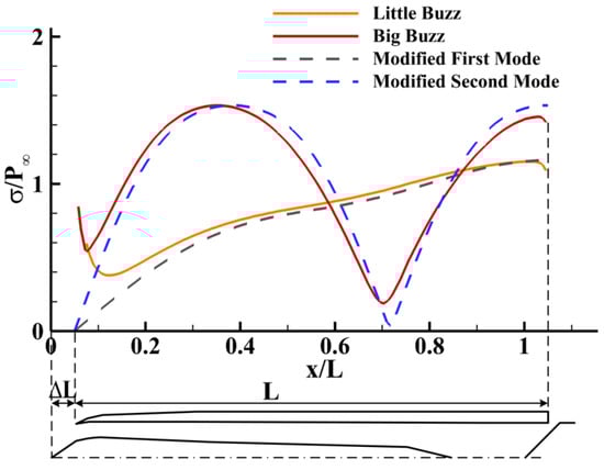
Figure 9.
Standard deviation curve of static pressure in inlet buzz and modified acoustic model.
It is worth noting that, ideally, for duct resonance, the standard deviation of sound pressure at the positions of nodes is zero, while in terms of inlet buzz, the standard deviation of nodes is not zero in spite of the minimum. The position of the second node on the big buzz curve is slightly ahead of x = 2/3·L and the distance between the node and the antinode in the inlet is not strictly a quarter wavelength. Besides the variation in the inlet geometry, the error mainly attributes to the viscous effects, which lead to the damping in the acoustic wave propagation. The acoustic theory applied in the duct is based on the inviscid assumption, while the viscous effects play an important role in the inlet buzz simulations [17].
The existence of damping is easy to understand above-mentioned discrepancies from the perspective of energy dissipation. (1) The pressure standard deviation at the node is not zero. The energy to sustain the inlet buzz is continuously dissipated due to the existence of damping. If there is no pressure fluctuation at the nodes, the periodic oscillation flow between two nodes could not be maintained because the energy would not be transferred through the node. (2) The amplitudes of each node and antinode are different along the axial direction of the inlet. The closer to the sound source, the larger the amplitudes of the node and antinode are, and their distribution is not strictly equidistant. The energy loss along the passage reduces the amplitude at the downstream node and antinode. Therefore, damping in fluid flows is an issue worthy of discussion.
5. Resonance under Jet Excitation and Damping Estimation
As a periodic oscillation phenomenon, inlet buzz is bound to have damping. However, the dynamic equation of the buzz system has not been established, and the damping of the fluid oscillation system has not been precisely defined. Therefore, it is extremely difficult to determine the relationship between damping and other variables. In this section, some quantitative calculations are carried out around the effect of viscous damping on pressure oscillations.
It is known that when the external excitation frequency is consistent with the natural frequency of the oscillatory system, the system shows a significant resonance characteristic. At this time, the external excitation has the greatest effect on the original oscillation system and the resonance response exhibits non-linear characteristics. In this paper, the resonance effect is considered to be equivalent to superimposing a nonlinear amplified excitation on the original oscillating system. The nonlinear amplification effect is related to damping and reflects the influence of damping on the strength of nonlinearity to some extent. From another perspective, the amplification effect in the resonance state may serve as a reference for estimating the magnitude of the damping.
According to the above idea, a periodic external excitation is required to be introduced into the original oscillation system. The numerical simulation of the oscillating system under excitation is conducted with the intention of achieving the resonance effect. It is worth mentioning that the acoustic model for the description of inlet buzz is based on the linear superposition of standing wave, however, the oscillatory system with consideration of damping is usually a nonlinear system. By comparing the results of the linear model and the nonlinear simulation, the nonlinear amplification effect could be obtained.
5.1. Excitation Results of Nonlinear Simulation
In order to prevent separation and suppress buzz oscillations, many methods of flow control are examined in various literature, such as boundary layer suction [29], bleeding and injection [30], and vortex generators [31]. Some new techniques, for example micro-vortex generator [32], plasma actuators [33], and cavity [34] are also verified to be effective. In present study, the purpose of introducing flow control method is to trigger resonance using an unsteady excitation. With this consideration, the method of bleeding and injection was chosen as the form of the periodic excitation for easy control of the excitation frequency.
The simulations of inlet buzz under excitation are based on the results of the little buzz and the big buzz. A small perturbation jet, as an external excitation, with different control parameters is introduced at the axial position of 0.059·L, where is a 2 mm jet slot. As shown in Figure 10, a periodic “mass-flow-inlet” boundary condition is imposed on the slot JK on the center body near the entrance of the inlet. The “mass-flow-inlet” boundary condition is given by a user-defined function (UDF) and it satisfies the cosinusoidal form:
where denotes the mass flow rate of the unsteady jet, represents the mean of the mass flow rate at the inlet exit, represents the jet frequency, and is a coefficient which represents the jet intensity and could be evaluated by the ratio of the jet amplitude to the mean of the mass flow rate at the inlet exit. is the phase difference between the unsteady jet and the standing wave in the original flow field. In the simulation, the jet amplitude () remains constant as 0.002, however, due to the is about 0.137 during little buzz and about 0.0998 during big buzz, correspondingly, the intensity coefficient is about 1.5% and 2%.
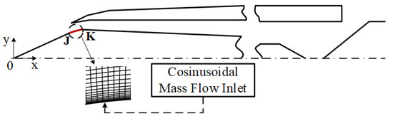
Figure 10.
Location of injection slot.
According to Equation (18), adjusting the parameters of small perturbation jet (e.g., , , ) may help to change the pressure oscillation inside the flow passage. In order to verify the excitation effect of resonance under the jet frequency of 120 and 360 Hz, comparing the cases under a non-natural-frequency jet is required. Keeping the jet intensity of = 1.5%, a jet with a frequency of 120 Hz but a different phase is used to trigger the little buzz resonance while two other jets of 80 and 160 Hz simulate the non-resonance state for comparison. Similarly, keeping = 2%, the jet of 360 Hz is aimed to trigger big buzz resonance, while the cases of 180 and 540 Hz are regarded as comparison groups.
The intensity of pressure oscillation in a one-dimensional continuous channel is described by the total of the standard deviations along the entire inlet, namely , and this sum represents the excitation effect under different jets to some extent. The intensity of oscillation () before introducing the perturbation jet would be used for normalization so that the excitation effect of enhancing or suppression could be judged by the normalized value (greater than 1 or less than 1).
Figure 11 shows the excitation effect of the little buzz under different-frequency jets. With the phase difference varying from 0 to 2π, the excitation effects show two types of trends. When the frequency of jet is identical to the natural frequency of the little buzz (120 Hz), the excitation effect fluctuates around the no-jet line, decreasing first and then increasing, reaching the minimum of 0.982 at π. The minimum means the little buzz is most suppressed at the phase difference of π. In contrast, when the jet frequency avoids the natural frequency of the little buzz, the trend of the excitation effect is closed to the horizontal no-jet line. The intensity of oscillation along the inlet is not significantly affected no matter the jet phase. Through the analysis of jet frequency and jet phase, it is considered that the resonance of the little buzz would appear when the jet frequency is 120 Hz and the phase difference is π. Figure 12 shows the case of big buzz and the description of Figure 12 is similar to that of the little buzz. The difference lies in the specific values, for example, the minimum at π is 0.947 in the resonance state of the big buzz. The different excitation effects may illustrate that the resonance of the big buzz is more significant than the little buzz under a jet with constant amplitude. So far, both the resonance simulations of little buzz and big buzz are obtained and verified.
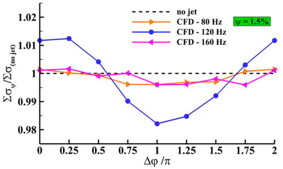
Figure 11.
Excitation effect of little buzz oscillation under different jet frequencies.
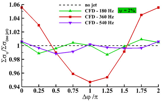
Figure 12.
Excitation effect of big buzz oscillation under different jet frequencies.
5.2. Nonlinear Amplification Effect and Pressure Oscillation Damping
The oscillation system under excitation is modeled further based on the linear superposition method. The perturbation jet at the entrance of the inlet is treated as an incoming wave. After reflecting back from the choked exit, a perturbation standing wave is formed. The pressure of the perturbation standing wave could be written as:
After linear superposition, the pressure of the little buzz and the big buzz under the jet of 120 and 360 Hz might be, respectively, expressed as:
According to Equations (20) and (21), in the resonance state, the oscillation intensities of the linear model and the nonlinear simulation are displayed in Figure 13. With regard to the result of the linear model, the perturbation standing wave of 120 Hz reduces the oscillation intensity of little buzz to 0.988 when the phase difference is π. In addition, for the case of the big buzz superposing the perturbation standing wave of 360 Hz, the minimum at π is 0.983, as shown in Figure 13. Although the trends of the linear model and the nonlinear simulation are consistent, the fluctuation amplitude of the excitation effect in the nonlinear simulation is significantly larger than that of the linear model.
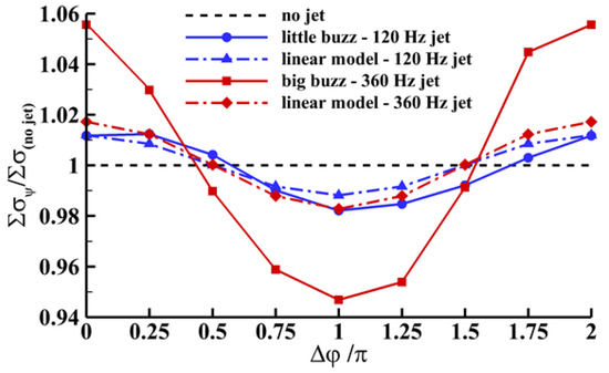
Figure 13.
Comparison between the linear model and the nonlinear simulation in the resonance states of the little buzz and the big buzz.
Regarding the discussion at the beginning of this section, the wide discrepancies may be attributed to the nonlinear amplification effect of resonance. The nonlinear amplification effect could be simply evaluated by the amplification factor M acting on the perturbation standing wave. Then the Equations (20) and (21) could be modified as
The amplification factor M may be determined in the comparison between the linear model and the nonlinear simulation. In order to match the fluctuation amplitude of the excitation effect, attention is focused on the minimum at the phase difference of π. For the little buzz, the minimum of the linear model and of the nonlinear simulation are about 0.988 and 0.982, respectively. The amplification factor M1 is set to be equal to (1 − 0.982)/(1 − 0.988) = 1.51 so that the two minimum points would coincide with each other. The oscillation intensities of the modified model at other phase conditions were recalculated, as shown in Figure 14. The same procedures were used in determining the M2 in the case of big buzz. Setting the M2 equal to (1 − 0.947)/(1 − 0.983) = 3.09, the results of the modified model are shown in Figure 14.
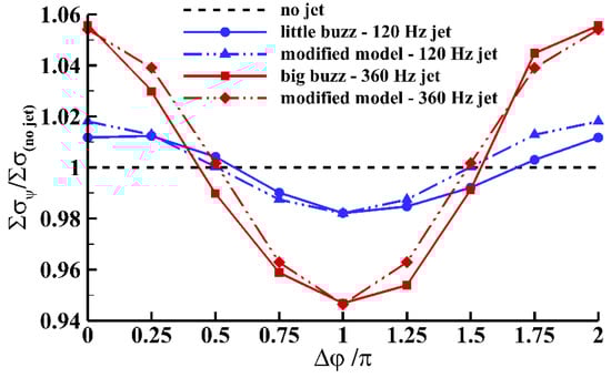
Figure 14.
Modified model and nonlinear simulation in the resonance states of the little buzz and the big buzz.
Based on the nonlinear amplification factor of pressure oscillations, the damping method for solid vibration was employed to calculate a pressure oscillation damping of a one-dimensional fluid system. The pressure oscillation damping is different from the traditional definition of damping, but it probably keeps the same variation trend and reflects the same physical meaning as the real damping.
In the case of small damping, the amplification ratio M in solid vibration has the following relationship with the frequency ratio and the damping ratio .
When the frequency ratio is 1, the damping ratio is equal to 1/(2M). Extending Equation (24) to this case of the pressure oscillation, the pressure oscillation damping of the little buzz and the big buzz are obtained as 0.33 and 0.16, respectively. It is concluded that the damping of the little buzz is greater than that of the big buzz. The higher the oscillation frequency, the smaller the pressure oscillation damping, which is consistent with the trend of damping discussed in solid vibration. Pressure oscillation damping as an estimate of the true damping may be reasonable.
The existing research suggests that inlet buzz is a self-excited oscillation, so the introduction of the excitation signal is equivalent to the forced vibration of a self-excited system. The descriptions of the related dynamic equations and the precise derivation of the nonlinear damping of this oscillation system are pending further study.
6. Conclusions
In this study, the inlet buzz phenomenon observed in Nagashima’s experiment was successfully reproduced by employing a two-dimensional dynamic mesh technique. The numerical results of both the little buzz and the big buzz were analyzed for the frequency characteristics and the pressure oscillatory characteristics. The little buzz contains the oscillation pattern of the big buzz, while some higher-frequency flow patterns may exist in the big buzz. In addition, pressure nodes and antinodes exist in the buzz pattern and the transient pressure oscillation of the little buzz and the big buzz are extremely similar to a standing wave with 1/4 and 3/4 wavelength, respectively.
The two types of the inlet buzz phenomenon were modeled mathematically based on a one-dimensional acoustic theory in which the internal flow passage of the supersonic inlet was simplified as a constant-section area duct with an open end and a closed end. Pressure variation in the duct was modeled as a synthesis of the incident and reflected wave. The frequency of inlet buzz is closely related to the resonant mode of the standing wave. The credibility of the acoustic model was validated in the comparison of the pressure standard deviation along the internal flow path. The acoustic model was further modified for a better agreement with the inlet buzz. The modified results indicate that standing waves of more than one frequency would be simultaneously excited during buzz, of which the energy of the dominant-frequency component accounts for the largest proportion. Neglecting a slight area variation of the inlet duct, the remaining discrepancies between the simulation and the ideal acoustic model might be attributed to the viscous damping in the fluid oscillation system.
With regard to the exploration of the damping, the inlet buzz systems under the excitation of different perturbation jets are involved. If the resonance could be triggered by the jet, the nonlinear amplification effect of resonance might be utilized to estimate the damping of the little buzz and the big buzz. The resonance results of the linear model and the nonlinear simulation were compared with each other and then the nonlinear amplification factor M of the little buzz and the big buzz were obtained as 1.51 and 3.09. The calculated pressure oscillation damping of the little buzz and the big buzz are 0.33 and 0.16, which could be regarded as an estimation of real damping.
Author Contributions
Conceptualization, J.Z.; methodology, J.Z.; software, J.Z. and W.L.; validation, W.L. and Y.W.; formal analysis, W.L. and J.Z.; investigation, W.L.; data curation, W.L.; writing—original draft preparation, W.L.; writing—review and editing, C.Y.; visualization, C.Y.; supervision, C.Y.; project administration, J.Z. and Y.Y.; resources, Y.Y.; funding acquisition, Y.Y. All authors have read and agreed to the published version of the manuscript.
Funding
This study was funded by the National Natural Science Foundation of China (No. 51906208 and No. 91941103), the Equipment Exploratory Research Fund (No. 61402060301), and the Weapon Exploratory Research Fund (No. 6141B010266).
Acknowledgments
The team members of School of Aerospace Engineering of Xiamen University are gratefully acknowledged.
Conflicts of Interest
The authors declare no conflict of interest.
References
- Chang, J.T.; Li, N.; Xu, K.J.; Bao, W.; Yu, D.R. Recent research progress on unstart mechanism, detection and control of hypersonic inlet. Prog. Aerosp. Sci. 2017, 89, 1–22. [Google Scholar] [CrossRef]
- McClinton, C.R.; Hunt, J.L.; Ricketts, R.H.; Reukauf, P.; Peddie, C.L. Airbreathing hypersonic technology vision vehicles and development dreams. In Proceedings of the 9th International Space Planes and Hypersonic Systems and Technologies Conference and 3rd Weakly Lonized Gases Workshop, Reston, VA, USA, 1–5 November 1999. [Google Scholar]
- Tan, H.J.; Guo, R.W. Experimental study of the unstable-unstarted condition of a hypersonic inlet at Mach 6. J. Propuls. Power 2007, 23, 783–788. [Google Scholar] [CrossRef]
- Oswatitsch, K. Pressure Recovery in Missile in Reaction Propulsion at High Supersonic Speeds; Report no: TM-1140; NASA: Washington, DC, USA, 1947.
- Ferri, A.; Nucci, L.M. The Origin of Aerodynamic Instability of Supersonic Inlets at Subcritical Conditions; Report no: RM-L50K30; NASA: Washington, DC, USA, 1951.
- Dailey, C.L. Supersonic Diffuser Instability Dissertation; California Inst. of Technology: Pasadena, CA, USA, 1954. [Google Scholar]
- Fisher, S.A.; Neale, M.C.; Brooks, A.J. On the Sub-Critical Stability of Variable Ramp Intakes at Mach Numbers around 2; Report. ARC-R/M-3711; National Gas Turbine Establishment: Fleet, UK, 1970. [Google Scholar]
- Nagashima, T.; Obokata, T.; Asanuma, T. Experiment of supersonic air intake buzz. In Space Aeronautics Research and Development Mechanism; Report No. 481; Institute of Space and Aeronautical Science: Tokyo, Japan, 1972; Volume 37, pp. 165–209. [Google Scholar]
- Trapier, S.; Duveau, P.; Deck, S. Experimental study of supersonic inlet buzz. AIAA J. 2006, 44, 2354–2365. [Google Scholar] [CrossRef]
- Trapier, S.; Deck, S.; Duveau, P. Delayed detached-eddy simulation and analysis of supersonic inlet buzz. AIAA J. 2008, 46, 118–131. [Google Scholar] [CrossRef]
- Lee, H.J.; Lee, B.J.; Kim, S.D.; Jeung, I. Flow characteristics of small-sized supersonic inlets. J. Propuls. Power 2011, 27, 306–318. [Google Scholar] [CrossRef]
- Soltani, M.R.; Sepahi-Younsi, J. Buzz cycle description in an axisymmetric mixed-compression air intake. AIAA J. 2016, 54, 1040–1053. [Google Scholar] [CrossRef]
- Chen, H.; Tan, H.J.; Zhang, Q.F.; Zhang, Y. Buzz flows in an external-compression inlet with partially isentropic compression. AIAA J. 2017, 55, 4288–4295. [Google Scholar] [CrossRef]
- Chen, H.; Tan, H.J.; Zhang, Q.F.; Zhang, Y. Throttling process and buzz mechanism of a supersonic inlet at overspeed mode. AIAA J. 2018, 56, 1953–1964. [Google Scholar] [CrossRef]
- Chen, H.; Tan, H.J. Buzz flow diversity in a supersonic inlet ingesting strong shear layers. Aerosp. Sci. Technol. 2019, 95, 105471. [Google Scholar] [CrossRef]
- Newsome, R.W. Numerical simulation of near-critical and unsteady, subcritical inlet flow. AIAA J. 1984, 22, 1375–1379. [Google Scholar] [CrossRef]
- Lu, P.J.; Jain, L.T. Numerical investigation of inlet buzz flow. J. Propuls. Power 1988, 14, 90–100. [Google Scholar] [CrossRef]
- Hankey, W.L.; Shang, J.S. Analysis of self-excited oscillations in fluid flows. In Proceedings of the 13th Fluid & Plasma Dynamics Conference, Reston, VA, USA, 14–16 July 1980; AIAA: Reston, VA, USA, 1980. [Google Scholar]
- Chima, R.V. Analysis of Buzz in a Supersonic Inlet; Report no: TM-2012-217612; NASA: Washington, DC, USA, 2012.
- Hong, W.; Kim, C. Computational study on hysteretic inlet buzz characteristics under varying mass flow conditions. AIAA J. 2014, 52, 1357–1373. [Google Scholar] [CrossRef]
- Chang, J.T.; Yu, D.R.; Bao, W. Mathematical modeling and rapid recognition of hypersonic inlet buzz. Aerosp. Sci. Technol. 2012, 23, 172–178. [Google Scholar] [CrossRef]
- Chang, J.T.; Wang, L.; Bao, W. Mathematical modeling and characteristic analysis of scramjet buzz. Proc. IMechE Part G J. Aerosp. Eng. 2014, 228, 2542–2552. [Google Scholar] [CrossRef]
- Yamamoto, J.; Kojima, Y.; Kameda, M.; Watanabe, Y.; Hashimoto, A.; Aoyama, T. Prediction of the onset of supersonic inlet buzz. Aerosp. Sci. Technol. 2020, 96, 105523. [Google Scholar] [CrossRef]
- Roe, P.L. Approximate Riemann solvers, parameter vectors, and difference schemes. J. Comput. Phys. 1981, 43, 357–372. [Google Scholar] [CrossRef]
- Van Leer, B. Towards the ultimate conservative difference scheme. 5. A second order sequel to Godunov’s methods. J. Comput. Phys. 1979, 32, 101–136. [Google Scholar] [CrossRef]
- Spalart, P.R.; Allmaras, S.R. A one-equation turbulence model for aerodynamic flows. In Proceedings of the 30th Aerospace Sciences Meeting & Exhibit, Reston, VA, USA, 6–9 January 1992; AIAA: Reston, VA, USA, 1992. [Google Scholar]
- Yoon, S.; Jameson, A. Lower-upper symmetric-Gauss-Seidel method for the Euler and Navier-Stokes equations. AIAA J. 1988, 26, 1025–1026. [Google Scholar] [CrossRef]
- Luo, W.G.; Wei, Y.Q.; Dai, K.; Zhu, J.F.; You, Y.C. Spatiotemporal Characterization and Suppression Mechanism of Supersonic Inlet Buzz with Proper Orthogonal Decomposition Method. Energies 2020, 13, 217. [Google Scholar] [CrossRef]
- Sepahi-Younsi, J.; Forouzi Feshalami, B.; Maadi, S.R.; Soltani, M.R. Boundary layer suction for high-speed air intakes: A review. Proc. IMechE Part G J. Aerosp. Eng. 2018, 233, 3459–3481. [Google Scholar] [CrossRef]
- He, Y.; Huang, H.; Yu, D. Investigation of boundarylayer ejecting for resistance to back pressure in an isolator. Aerosp. Sci. Technol. 2016, 56, 1–13. [Google Scholar] [CrossRef]
- Titchener, N.; Babinsky, H. Shock wave/boundary layer interaction control using a combination of vortex generators and bleed. AIAA J. 2013, 51, 1221–1233. [Google Scholar] [CrossRef]
- Panaras, A.G.; Lu, F.K. Micro-vortex generators for shock wave/boundary layer interactions. Prog. Aerosp. Sci. 2015, 74, 16–47. [Google Scholar] [CrossRef]
- Lapushkina, T.A.; Erofeev, A.V. Supersonic flow control via plasma, electric and magnetic impacts. Aerosp. Sci. Technol. 2017, 69, 313–320. [Google Scholar] [CrossRef]
- Karbasizadeh, M.; Babaei, A.R.; Bazazzadeh, M. Optimization of slot geometry in shock wave boundary layer interaction phenomenon by using CFD– ANN–GA cycle. Aerosp. Sci. Technol. 2017, 71, 163–171. [Google Scholar] [CrossRef]


© 2020 by the authors. Licensee MDPI, Basel, Switzerland. This article is an open access article distributed under the terms and conditions of the Creative Commons Attribution (CC BY) license (http://creativecommons.org/licenses/by/4.0/).