A Fuzzy Unscented Kalman Filter in the Adaptive Control System of a Drive System with a Flexible Joint

Abstract

This paper presents an application of an Unscented- and a Fuzzy Unscented- Kalman Filter (UKF and FUKF) to the estimation of mechanical state variables and parameters in a drive system with an elastic connection. The cascade control structure incorporating an IP controller supported by two additional feedbacks and suitable adaptation mechanism is investigated in this study. The coefficients of the control structure are retuned on the basis of the value of mechanical parameters estimated by filter. The effectiveness of the proposed approaches (classical and fuzzy) is researched through simulation and experimental tests.

1. Introduction

Due to the growing demand for high performance drives, the problem of precision control has become a prevalent research subject. How to control mechatronic systems in an accurate way is a crucial issue in industry, the problem appearing in traditional conveyer and rolling-mill drives, paper machines, robot arm drives, CNC machines, or MEMS (micro-electromechanical systems), etc. [1,2,3,4,5,6,7,8,9,10]. When designing an advanced drive system, one should take into consideration all factors that can potentially affect the performance of the control, including the mechanical characteristics of the drive, especially the finite stiffness of the shaft. A factor which may have negative impact on the performances of a mechatronic drive is the variation of the plant parameters. In order to compensate the mentioned factors, a suitable control algorithm has to be introduced [1,2,3,4,5,6,7,8,9,10,11,12,13,14,15,16,17,18,19].

Different control concepts have been proposed over the last few decades in order to improve the performance of the drive with a flexible connection. The basic works concern the application of the simple PI/PID controller [9]. The effectiveness of this simple structure can be improved by a proper location of the system poles. A more advanced concept relies on Resonance Ratio Control (RRC) [10,12]. However, the damping ability of this method is also limited. A comparative analysis of the system with a PI controller with various additional feedbacks, is shown in [9]. It is proven that inclusion of two additional feedbacks allows one to put the poles of closed-loop system in the required position. A similar performance is ensured by the structure with a state controller or Forced Dynamic Control algorithm. There are also much more advanced control algorithms used for damping oscillations in e elastic drive systems, for example sliding mode control [1,13,16,20], which is especially suitable for the plant with changeable parameters. Over the last few decades the model predictive control (MPC) concept has gained a lot of attention. There are also works concerning the application of this algorithm for a drive system with a flexible joint [21,22]. For the plant with changeable parameters the concept of adaptive control is also suitable. It ensures the desired responses of the system despite any changes of its parameters. In [11,14,17,23,24,25] direct and indirect approaches are presented.

The suitable selection of one of the abovementioned control algorithms depends on the design requirements. The best control performance can be ensured by using advanced control methodologies, however, they require knowledge of the state variables of the object and additionally about the values of changeable parameter(s). Therefore, a suitable estimation algorithm is needed [26,27,28,29,30].

Among the most popular estimation techniques used for a two-mass system two main groups can be listed [24,30]. Methods based on the mathematical model of the plant, e.g. the Luenberger observer, belong to the first framework. The Luenberger observer has a simple control structure, where the gains of the estimator can be determined using the algebraic method. However, it has to be mentioned that in this system the robustness to the measurements and plant noises is limited. In the literature different modifications which can improve the performance of this estimator can be found. In [31] an additional fuzzy system is applied which improved the estimation quality. The next framework relies on the Kalman filter algorithm, in which two main approaches can be distinguished, namely the Extended and Unscented Kalman Filters [19,29,30,31]. The Kalman filters are said to be robust against measurements and process noises. However, noises should be white and have a Gaussian character, which is usually not fulfilled in industrial applications. In [32] a comparative analysis between the Kalman filter and Luenberger observer is performed. It is proven that the Kalman filter, as expected, is more robust to the noises and can provide more accurate state estimations. The modification of the standard EKF algorithm based on the suitable retuning of the values of the covariance matrix is shown in [24]. The proposed approach confirms its effectiveness. The application of UKF in the field of mechatronic control is less popular due to the more complicated algorithm compared to EKF. The other algebraic method is the moving horizon estimator. The estimator is based on the present and limited number of the past samples. This improves its robustness to random noises. However, its application to drive control is limited due to the very complicated numerical algorithm. The second main framework relies on artificial intelligence (AI) techniques. The following approaches can be distinguished: those relying on neural networks, fuzzy logic and gray estimators [33,34,35]. These methodologies do not need information about the mathematical model of the plant, and only training data registered for different operation conditions are necessary. Despite their good performance, pure artificial intelligence-based methodologies are not popular in industry.

Fuzzy logic systems have become extremely popular in recent years. They are used in different branches of industry, including automation control and drive systems. Fuzzy logic-motivated structures can play a role as a controller, compensator or additional element. Generally, they have the ability to express different difficult relationships which are not easy to formulate using classical logic. They can be used as a separate estimator or as an additional part supporting a classical estimator.

Different techniques, including AI-based ones, in order to improve the KF performance have been reported in the literature. In [36] the authors considered a navigation system based on standard and extended KF. In the paper the tuning of the KF by a fuzzy-logic-based system is proposed. The additional logical mechanism allows adaptation to the sensor noise characteristics. A novel scheme called the adaptive fuzzy strong tracking Kalman filter is proposed in [37] for a navigation system. In order to improve the KF performance the fuzzy system based on TSK model is proposed. The authors report good performances of the considered system. The implementation of the UKF in a ship positioning system is reported in [38]. In order to improve the performance of the UKF in the presence of time varying noises, model mismatch and drift forces an adaptation mechanism is proposed. It adopts the parameters of the noise covariance based on residual covariance matching methods. The proposed system ensures better stability and accuracy compared to the traditional one. Issues relevant to fault detection and diagnosis of wind turbines are presented in [39]. The KF is applied in order to estimate selected parameters of the plant. The fuzzy fading algorithm adopts the KF, which allows one to improve the quality of fault parameter detection. The application of the UKF supported by a fuzzy adaptive system in a cognitive radio networks is presented in [40]. The UKF is implemented to minimize the mean square estimation errors. The fuzzy system detects the licensed primary user. The proposed scheme allows one to achieve better detection gains. It also ensures a lower global probability of error as compared to conventional systems. The application of neural networks with different KF algorithms is also a popular target. In [41] a GPS system is considered. Three UKF filters with different noise covariance are implemented simultaneously. The soft switching algorithm is proposed to adopt to the actual characteristics of noises. The difference between particular UKFs generates data for a grey neural network. This system is used to predict and compensate position errors when the GPS system is blocked. The issues related to flood forecasting with accordance of KF and NN are reported in [42]. The UKF is used to model the point forecasts obtained from recurrent and static neural networks. The combination of both methods allows one to increase the accuracy of the prediction. In the literature, there are a number of examples of application of the UKF in different industrial branches. However, within the area of mechatronic systems these applications are rather rare [43,44]. Works showing experimental validation of different UKF algorithms in the adaptive control structure of two-mass system seem to be expected by specialists. This is the main motivation for the authors.

In this study the fuzzy UKF is proposed to determine the mechanical state variables of the elastic system and the value the load machine’s mechanical time constant. Contrary to [45], where the classical UKF was discussed, in the present paper a combination of the UKF with a fuzzy system is considered. The following variables are used as an input variables of the fuzzy system: the load machine’s time constant (estimated value), the electromagnetic torque and the estimated shaft torque. In accordance with the variations of those variables, the values of the covariance matrices of UKF are retuned on-line, which ensures the improvement of the estimation accuracy. The applied fuzzy system allows us to improve the estimation accuracy of the UKF for different plant parameters as well as in dynamic states. A critical comparative analysis between the classical UKF and the proposed solution is also one of the main points of this work.

The paper consists of five sections. The first one introduces the problem, and the following provides a brief description of the mathematical model of the plant. In the next section the adaptive control structure with an IP controller and feedbacks from the selected states: shaft torque and difference between the system’s speeds is introduced. This structure, described in [46], has good torsional vibration damping properties. The feedback from estimated load torque is included into the considered control structure. Then the classical UKF and fuzzy UKF are described in detail. The comparative analysis between these two structures is the main point of the work. The effectiveness of the considered control algorithm is checked in a simulation as well as experimental study. The paper is concluded with some remarks summarizing the findings.

2. Mathematical Model of the Plant and Adaptive Control Structures

In scholarly papers, a variety of mathematical models are used when analyzing plants with elastic couplings. Generally, the drive system can be modeled as a two-mass system [47]. The inertia of the shaft is divided by half and added to both sides—later it is regarded inertia-free. In the final model the first mass serves as the moment of inertia of the drive and half of the shaft and the second mass refer to the moment of inertia of the load side and additional half of shaft. The internal damping of the shaft is usually omitted. This simple model is used in more than 99% of papers describing the control of different plants (starting from traditional rolling mill drives, through servo-drive, robot arm drives, ending on hard-disc drive). It results from the following factors. Firstly, in a real-time application with small time constant, there is a need to use the model in which the states can be calculated very fast. This is especially important for systems working with different types of observers. Also, for systems designated for industrial application, where standard controllers (PI, states or even predictive) are used, only models with a few states can be implemented. A complicated model with many states is not suitable for control engineers. The following state equation is a characterization of the described system (non-linear friction has been neglected) [24]:

$$\frac{d}{dt}\left[\begin{array}{c}{\omega }_1\left(t\right)\\ {\omega }_2\left(t\right)\\ m_s\left(t\right)\end{array}\right]=\left[\begin{array}{ccc}0& 0& \frac{-1}{T_1}\\ 0& 0& \frac{1}{T_2}\\ \frac{1}{T_c}& \frac{-1}{T_c}& 0\end{array}\right]\left[\begin{array}{c}{\omega }_1\left(t\right)\\ {\omega }_2\left(t\right)\\ m_s\left(t\right)\end{array}\right]+\left[\begin{array}{c}\frac{1}{T_1}\\ 0\\ 0\end{array}\right]\left[m_e\right]+\left[\begin{array}{c}0\\ \frac{-1}{T_2}\\ 0\end{array}\right]\left[m_L\right]$$

(1)

where: ω₁, ω₂—the speeds of driving and load side respectively, m_e, m_s, m_L—the electromagnetic, coupling, and disturbance torques, T₁, T₂—mechanical time constant of the driving and load side, T_c—the parameter which represents the elasticity of a coupling.

The two-mass drive mechanical model is only a simplification of the real-life system. Additional factors such as the nonlinear characteristic of the mechanical connection (including mechanical hysteresis) non-linear friction located on both sides, the imperfections in generated electromagnetically torque (for examples the torques ripples) and others influence the control properties. All these factors decrease the effectiveness of classical estimation techniques. Those factors motivate the search for different techniques. The presented model is suitable for any system where the moment of inertia of the elastic connection is much smaller compared to the moment of the inertia of the driving and the load machines. Otherwise, a more complicated model should be considered, such as a wave model [48]. The suitable selection of the model to be used is a compromise between the computational complexity and accuracy. It also has to be noted that for real-time applications the presented model is especially suitable due to its computational simplicity.

The control structure for an electrical drive comprises two major loops. The inner loop consists of a torque controller, suitable converter, an electromagnetic section of the driving engine and sensor(s) of current. A model of a torque loop can be obtained by theoretical considerations or by experimental identification [49,50]. Theoretical considerations may include a number of non-linear phenomena occurring in the control system of the converter (e.g. dead time), current measurement errors related to non-symmetrical power supply of current sensors, A/C sensor scaling errors [51], as well as the discreet effect of current measurement and control. In simulation models of different motor types (DC, PMSM, ACIM), the windings are assumed to be symmetrical, the resistance and inductance are constant, magnetic circuits are linear (saturation, hysteresis phenomena and eddy currents are omitted). The model substitute delay can be calculated as the sum of partial delay times, such as the calculation time of the controller, delay the anti-aliasing current filter, communication delay. Assuming that the drive will not operate in the second speed control zone, the simulation model of the engine and the converter for preliminary analysis and synthesis is simplified significantly. A detailed analysis of the modelling of these phenomena in the article is not needed because it does not affect the quality of control. Only experimental verification on a laboratory stand can confirm the validity of the assumed assumptions, which is presented the article. 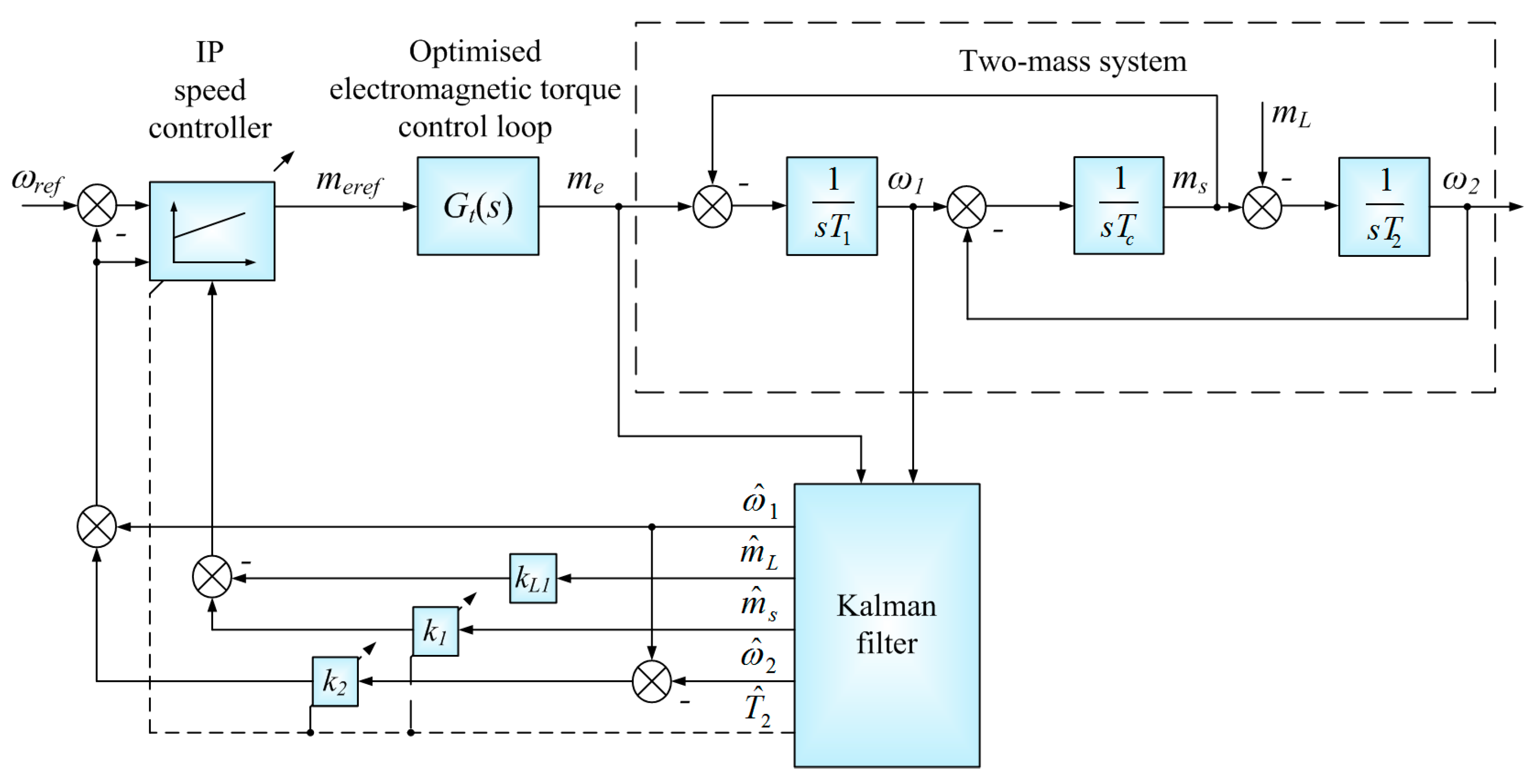Based on [49,50], the optimized torque control loop (Figure 1) can be replaced by the 1st order inertia. The gains of the controller are selected so as to provide a rapid torque control. Theoretically, the time constant of the electromagnetic part of the motor can be compensated, and only a small time constant of the power converter determines characteristics of the torque control structure. If the dynamics of the torque loop is not fast enough, two possible solutions can be applied. Firstly, the dynamics of the torque control loop can be included in the model of the plant and then used in control algorithm. In this case, the particular properties of the torque loop are not important because its dynamics is taken into account. Secondly, the dynamics speed control can be decreased, yet is it not preferable solution in high-performance drive. In the present work the torque control loop is equivalent to the first order term, the time constant of which is set to 1.5 ms. This means that the inner loop dynamics are much faster as compared to those of the speed loop.

The basic structure with feedback from the motor speed does not ensure good dynamic characteristics of the system. To improve the dynamical characteristics of the drive, their modification is necessary. In this study the system with an IP controller supported by the additional feedbacks from the torsional torque and the difference between the driving motor and load machine speeds is considered. The coefficients of the control structure are calculated with the help of pole-placement, presented in [24], on the basis of the following formulas:

$$k_i={\omega }_0^4{T}_1{T}_2{T}_c$$

(2)

$$k_p=4{\xi }_r{\omega }_0^3{T}_1{T}_2{T}_c$$

(3)

$$k_2={\left({\omega }_0^2{T}_2{T}_c\right)}^{-1}-1$$

(4)

$$k_1=T_1{T}_2^{-1}\left(4{\xi }_r^2-k_2\right){\left(1+k_2\right)}^{-1}-1$$

(5)

$$k_{L1}=T_c{k}_i\left(1+k_2\right)+1+k_1$$

(6)

where: ω₀—the required frequency of the drive system poles, ξ_r—damping coefficient, k₁, k₂, k_i, k_p—feedback’s gains. The speed controller is described as:

$$G_r=k_p+\raisebox{1ex}{$k_i$}\!\left/ \!\raisebox{-1ex}{$s$}\right.$$

(7)

The considered control structure is presented in Figure 1.

To apply the adaptive control structure shown in Figure 1 the estimation of changeable parameter(s) is necessary—in the analyzed case the time constant of the load machine T₂. Therefore, the original state vector of the system is extended by an additional element 1/T₂. The feedback from the estimated load torque, evident in the control structure, is used to refine the drive characteristics with respect to variations of the load torque. The possible changes of stiffness coefficient of the elastic joint T_c can be used for monitoring purposes. However, the further extension of the state vector is not possible due to the fact that the observability condition will be not fulfilled, so the actual state vector cannot be extended. If this parameter has to be estimated, one of the additional states (load torque or time constant of the load machine) should be replaced by T_c, but this is outside the scope of this paper.

3. Classical and Fuzzy UKF Algorithms

Considering all possible state variable of presented above system it is possible to extend state vector by parameter. The classical two-mass system described by Equation (1) has been extended by additional disturbance m_L and parameter (time constants) 1/T₂. State vector of estimation system takes the form of Equation (8):

$$x_R\left(t\right)={\left[{\omega }_1\left(t\right)\begin{array}{c}\end{array}{\omega }_2\left(t\right)\begin{array}{c}\end{array}{m}_s\left(t\right)\begin{array}{c}\end{array}{m}_L\left(t\right)\begin{array}{c}\end{array}\frac{1}{T_2}\left(t\right)\right]}^T$$

(8)

The state space system with extended, nonlinear state and output equations can be written in the following form:

$$\frac{d}{dt}{x}_R\left(t\right)=A_R\left(\frac{1}{T_2}\left(t\right)\right)x_{\mathbf{R}}\left(t\right)+B_{R}u\left(t\right)+w\left(t\right)=f\left(x_R\left(t\right),u\left(t\right)\right)+w\left(t\right),$$

(9)

$$y_R\left(t\right)=C_R{x}_R\left(t\right)+v\left(t\right)$$

(10)

where system matrices may be defined as follows (in [p.u.]):

$$A_R\left(\frac{1}{T_2}\left(t\right)\right)=\left[\begin{array}{ccccc}0& 0& \frac{-1}{T_1}& 0& 0\\ 0& 0& \frac{1}{T_2}\left(t\right)& \frac{-1}{T_2}\left(t\right)& 0\\ \frac{1}{T_c}& \frac{-1}{T_c}& 0& 0& 0\\ 0& 0& 0& 0& 0\\ 0& 0& 0& 0& 0\end{array}\right],B_R=\left[\begin{array}{c}\frac{1}{T_1}\\ 0\\ 0\\ 0\\ 0\end{array}\right],C_R={\left[\begin{array}{c}1\\ 0\\ 0\\ 0\\ 0\end{array}\right]}^T$$

(11)

and w(t), v(t)—represent process and measurement noises.

Based on above assumption (8), the matrix A_R depends on the parameter T₂, should be updated due to the estimation. The input and the output vectors of the electric servo drive are one element, for input the electromagnetic torque and motor speed as an output:

$$u=m_e, y={\omega }_1$$

(12)

The unscented Kalman filter [45,52] discrete function description can be presented as set of follow steps:

(1) Generation of sigma points and their weights:

$${\mathsf{\chi }}_{k-1|k-1}^{\left(0\right)}={x_R}_{k-1|k-1};W_s^{\left(0\right)}=\frac{\lambda }{L+\lambda }$$

(13)

$${\mathsf{\chi }}_{k-1|k-1}^{\left(i\right)}={x_R}_{k-1|k-1}+{\left(\sqrt{\left(L+\lambda \right)P_{k-1|k-1}}\right)}_i,i=1,\dots ,L;W_c^{\left(i\right)}=\frac{\lambda }{L+\lambda }+\left(1-{\alpha }^2+\beta \right)$$

(14)

$${\mathsf{\chi }}_{k-1|k-1}^{\left(i\right)}={x_R}_{k-1|k-1}-{\left(\sqrt{\left(L+\lambda \right)P_{k-1|k-1}}\right)}_{i-L},i=L+1,\dots ,2L;W_s^{\left(i\right)}=W_c^{\left(i\right)}=\frac{1}{2\left(L+\lambda \right)}$$

(15)

The probability distribution is described by a Gaussian random variable represented by deterministically appointed weighted sigma points. These points are subject to nonlinear transformations based on the dynamics model and observation of the considered object. The number of sigma points in the simplest version of this algorithm is (n + 1), and in typical solutions it is equal to (2n + 1).

(2) Nonlinear transformation of 2n + 1 sigma points according to the model of dynamic:

$${\mathsf{\chi }}_{k|k-1}^{\left(i\right)}=f_R\left({\mathsf{\chi }}_{k-1|k-1}^{\left(i\right)}\right),i=0,\dots ,2L$$

(16)

(3) Prediction of the state vector:

$${{\widehat{\mathbf{x}}}_R}_{k|k-1}={{\displaystyle \sum }}_{i=0}^{2L}{W}_s^{\left(i\right)}{\mathsf{\chi }}_{k|k-1}^{\left(i\right)}$$

(17)

(4) Prediction of the covariance matrix:

$$P_{k|k-1}={{\displaystyle \sum }}_{i=0}^{2L}{W}_c^{\left(i\right)}\left[{\mathsf{\chi }}_{k|k-1}^{\left(i\right)}-{{\widehat{\mathbf{x}}}_R}_{k|k-1}\right]{\left[{\mathsf{\chi }}_{k|k-1}^{\left(i\right)}-{{\widehat{\mathbf{x}}}_R}_{k|k-1}\right]}^T+Q_{k-1}$$

(18)

(5) Prediction of the output vector:

$${{\widehat{\mathbf{y}}}_R}_k={{\displaystyle \sum }}_{i=0}^{2L}{W}_s^{\left(i\right)}{C_R}_k{\mathsf{\chi }}_{k|k-1}^{\left(i\right)}$$

(19)

(6) Prediction of the mutual covariance matrices:

$$P_{x_k{y}_k}={{\displaystyle \sum }}_{i=0}^{2L}{W}_c^{\left(i\right)}\left[{\mathsf{\chi }}_{k|k-1}^{\left(i\right)}-{{\widehat{\mathbf{x}}}_R}_{k|k-1}\right]{\left[{C_R}_k{\mathsf{\chi }}_{k|k-1}^{\left(i\right)}-{{\widehat{\mathbf{y}}}_R}_k\right]}^T$$

(20)

$$P_{y_k{y}_k}={{\displaystyle \sum }}_{i=0}^{2L}{W}_c^{\left(i\right)}\left[{C_R}_k{\mathsf{\chi }}_{k|k-1}^{\left(i\right)}-{{\widehat{\mathbf{y}}}_R}_k\right]{\left[{C_R}_k{\mathsf{\chi }}_{k|k-1}^{\left(i\right)}-{{\widehat{\mathbf{y}}}_R}_k\right]}^T+R_k$$

(21)

(7) Calculation of resulting the Kalman filter gain:

$$K_k=P_{x_k{y}_k}{P}_{y_k{y}_k}^{-1}$$

(22)

(8) Correction of the state vector:

$${{\widehat{\mathbf{x}}}_R}_k={{\widehat{\mathbf{x}}}_R}_{k|k-1}+K_k\left[{y_R}_k-{{\widehat{\mathbf{y}}}_R}_k\right]$$

(23)

(9) Correction of the covariance matrix:

$$P_{k|k}=P_{k|k-1}-K_k{P}_{y_k{y}_k}{K}_k^T$$

(24)

(10) Return to the first step.

The values of the covariance matrices Q and R have to be determined in order to ensure the proper working of the UKF. However, in most industrial applications they are not accessible and have to be defined. Two main frameworks can be used for this purpose. The first group contains strictly mathematical methods like Bayesian, maximum likelihood, covariance matching, and preliminary correlation techniques. The second approach is based on known global optimization techniques, where the artificial intelligence methods are especially useful. In this approach parameters of the covariance matrices (Q and R) are determined on the basis of minimization between the real and estimated variables of the system.

In order to determine the values of the KF using genetic algorithm the following frameworks can be used. The first approach relies on the careful modelling of the plant including the characteristic of noises. Because the laboratory set-up is known quite accurately and the hypothetical transients of the system can be registered off-line, there is a possibility to determine its parameters. This approach requires deeper theoretical knowledge about noises. Nowadays, the covariance can be calculated using available software. This approach can also be implemented in an alternative way. To the optimisation procedure the simulation as well as experimental data, recorded off-line, should be used. The problem which is generally evident, results from the fact that not all system states are measured in a practical system (in the ring described in the paper only current and speeds are measured). Still combining the simulation and experimental data provides satisfactory results. The additional problem which appears here is a necessity for changing the form of cost function in order to include the simulation (all states available) and experimental data (limited states available). In our opinion this approach ensures the best possible values for specific set-up.

The second approach is much more general. As in the previous case, the mathematical model of the plant is used to generate the transients of the system states. However, contrary to the above-presented case, assumed noises are bigger than in existing set-up. This limits the possible performance of the KF. However, the obtained system is much more robust to changes in a real plant. This approach is more save and guarantee proper operation of the closed-loop control structure. Still, the performance of the estimator is not fully optimal for the particular plant. This approach is implemented in the paper.

In the current work elements of the covariance matrices Q and R are preliminary choosed off-line with the help of genetic algorithm with the use of following cost function:

$$F=\frac{1}{n}(\delta {\omega }_1·\dot{\delta }{\omega }_1·\delta {\omega }_2·\dot{\delta }{\omega }_2·\delta m_s·\dot{\delta }{m}_s·\delta m_L·\dot{\delta }{m}_L·\delta T_2·\dot{\delta }{T}_2)$$

(25)

where:

$$\delta x={{\displaystyle \sum }}_{i=1}^n\left|x_i-{\widehat{x}}_i\right|$$

(26)

$$\dot{\delta }x=\frac{{{\displaystyle \sum }}_{i=1}^n\left|\left(x_{i+1}-{\widehat{x}}_{i+1}\right)-\left(x_i-{\widehat{x}}_i\right)\right|}{T_s}$$

(27)

where: n—total number of samples, x, $\widehat{x}$—real and estimated variables, T_s—the sampling step.

In the cost function not only the estimation errors of all considered variables are important but also its derivatives with direction are allowed. This approach allows obtaining smoother. The best solutions of diagonal Q and matrix R elements of found are shown in

Table 1. Values of the covariance matrices Q and R selected by genetic algorithm.

q11	q22	q33	q44	q55	R
4.0	1.75E-6	3216.43	8868.68	15464.26	101983.79

.

In order to improve the estimation accuracy of the presented UKF algorithm the following refinement based on fuzzy techniques is proposed. Such structure of additional fuzzy system used for dynamic tuning is presented in Figure 2. The system is based on the following rules (for simplicity of the presentation only examples for one element is shown):

$$\begin{array}{l}R1:IF\left({\widehat{T}}_{2}isS\right)THEN\left(q_{11}is{q}_{11ss}\right)\\ R2:IF\left({\widehat{T}}_{2}isS\right)AND\left(S_{out}isF\right)THEN\left(q_{11}is{q}_{11ds}\right)\\ R3:IF\left({\widehat{T}}_{2}isB\right)THEN\left(q_{11}is{q}_{11sb}\right)\\ R4:IF\left({\widehat{T}}_{2}isB\right)AND\left(S_{out}isF\right)THEN\left(q_{11}is{q}_{11db}\right)\end{array}$$

where: $\widehat{T_2}$—the estimated value of the mechanical time constant of the load machine, q₁₁, q_11ii—the initial and optimal value of covariance matrix element.

In order to decrease the computational complexity of the system, the defuzzyfication strategy based on the commonly used singleton method is selected in the paper. The characteristic feature of this method relies on the replacement of traditional fuzzy membership function by singleton values. Those singletons are placed in the point where the traditional membership functions have maximal values. The output of the system is calculated with the help of following equation:

$$y=\frac{{{\displaystyle \sum }}_{i=1}^m{y}_i{\mu }_{Ai}}{{{\displaystyle \sum }}_{i=1}^m{\mu }_{Ai}}$$

(28)

where: y_i—value of i-th of the singleton value, m—number of rules, μ_Ai—activation level of the i-th rule prerequisite.

The following feature can be accurate in this system. It is based on three inputs. The first one is an estimated value of the time constant of load machine. The values of Q and R are computed in a fuzzy system due to the present value of $\widehat{T_2}$ in order to keep estimation accuracy. Two other inputs generate a signal S_out which is the modulus of the electromagnetic and shaft torque difference. This allows detecting the present static and dynamic states of the system. The resulting gain of the UKF should be smaller in order to avoid noises during steady state. However, in dynamic states (during motor start-up, reversal, application of the load torque) the resulting gains of the UKF may be increased in order to minimize estimation errors faster. The values of singletons in fuzzy system have been selected using genetic algorithm with known cost function (25). The effectiveness of proposed method will be shown in the next section.

According to the literature different approaches can be implemented in order to determine the structure and parameters of the fuzzy supporting system. One of the most popular is based on selected fuzzy clustering algorithms. Most of them are dependent on distance criteria. In a fuzzy clustering algorithm one sample can belong to many sets, contrary to classical clustering approaches. The data point which is located closer to the center of the cluster has a bigger degree of belonging to this cluster as compared to the data point located farer. The fuzzy c-means algorithm is a well-established procedure used in many papers. It utilizes reciprocal distance in order to calculate fuzzy weights. Despites its obvious advantages, the fuzzy clustering technique also has some drawbacks. The most significant one is its computational requirements for complex systems. Additionally, the generated system can be relatively big, which can cause computational problems in real-time applications. Due to that reason this methodology was not used in the paper.

In the current studies the structure and parameters of the fuzzy system are selected on the basis of two methodologies, i.e. human experience and, for limited parameters, genetic algorithms. Firstly the input signals of the fuzzy system are selected. Then the structure, type and location of membership functions are specified. One of the requirements is to design a system which can be working in real-time application. Therefore, the proposed system has relatively small number of parameters. The input membership functions influence the characteristics of the system significantly, For that reason only they are selected to optimization procedure based on GA. The values of singletons in the fuzzy system have been selected using genetic algorithm with a known cost function (25). Because the obtained results are satisfactory, the other parameters (input membership function) were not changed. However, it should be stressed that optimization of all system parameters can further improve the effectiveness of the system.

4. Results

In the simulation test the effectiveness of the classical and fuzzy UKF is investigated. the structure of adaptive control shown in Figure 1 is considered. According to the description provided in the previous session, on the basis of the electromagnetic torque and the motor speed (disturbed in simulation by noises), the system state variables are reconstructed. To determine the estimated value of the time constant of the load torque is utilized updating of the control structure factor. Additionally, the elements of the covariance matrices are modified by the fuzzy system.

Firstly, the classical UKF is tested. In Figure 3 the transients process of the actual and estimated variables, as well as its estimation error are presented. The motor drive system that is being considered at work is tested under reverse conditions. The drive system started with the correct value of the mechanical time constant of the load T₂ = 203 ms (Figure 3i). Then, this parameter starts to vary at the time t = 8.5, 17.5, and 26.5 s to reach the following values: 406, 609 and 812 ms, respectively. The load torque is activated and deactivated periodically (Figure 3h). The following cyclical operation made it possible to test the quality of the estimated variables under various conditions. The adaptive system working with the UKF operates correctly.

Next the FUKF is examined. The conditions of tests are identical as for the UKF. The real and estimated transients process of this system are shown in Figure 4. As expected the system operates correctly. The biggest visible difference between the two systems is evident in the transients’ process of the mechanical load time-constant of the machine (Figure 3i and Figure 4i).

In order to evaluate the estimation quality normalised values of estimation errors and their derivatives for individual variables are presented in the

Table 2. Values of the estimation errors and their derivatives for the UKF and FUKF—simulation study.

Algorithm	$\frac{\mathit{\delta }{\mathit{\omega }}_{\mathbf{1}}}{\mathit{n}}$	$\frac{\mathit{\delta }{\mathit{\omega }}_{\mathbf{2}}}{\mathit{n}}$	$\frac{\mathit{\delta }{\mathit{m}}_{\mathit{s}}}{\mathit{n}}$	$\frac{\mathit{\delta }{\mathit{m}}_{\mathit{L}}}{\mathit{n}}$	$\frac{\mathit{\delta }{\mathit{T}}_{\mathbf{2}}}{\mathit{n}}$	$\frac{\dot{\mathit{\delta }}{\mathit{\omega }}_{\mathbf{1}}}{\mathit{n}}$	$\frac{\dot{\mathit{\delta }}{\mathit{\omega }}_{\mathbf{2}}}{\mathit{n}}$	$\frac{\dot{\mathit{\delta }}{\mathit{m}}_{\mathit{s}}}{\mathit{n}}$	$\frac{\dot{\mathit{\delta }}{\mathit{m}}_{\mathit{L}}}{\mathit{n}}$	$\frac{\dot{\mathit{\delta }}{\mathit{T}}_{\mathbf{2}}}{\mathit{n}}$
	(p.u.)	(p.u.)	(p.u.)	(p.u.)	(s)	(p.u.)	(p.u.)	(p.u.)	(p.u.)	(s)
UKF	0.0013	0.0020	0.0212	0.0332	0.0182	0.1893	0.1343	1.8868	1.7408	0.1364
FUKF	0.0007	0.0013	0.0154	0.0259	0.0123	0.1576	0.1263	1.5264	1.5664	0.1035

. In

Table 3. Values of the percentage differences of the estimation errors and their derivatives for the FUKF in relation to the UKF—simulation study.

Algorithm	${\mathit{a}}_{\frac{\mathit{\delta }{\mathit{\omega }}_{\mathbf{1}}}{\mathit{n}}}$	${\mathit{a}}_{\frac{\mathit{\delta }{\mathit{\omega }}_{\mathbf{2}}}{\mathit{n}}}$	${\mathit{a}}_{\frac{\mathit{\delta }{\mathit{m}}_{\mathit{s}}}{\mathit{n}}}$	${\mathit{a}}_{\frac{\mathit{\delta }{\mathit{m}}_{\mathit{L}}}{\mathit{n}}}$	${\mathit{a}}_{\frac{\mathit{\delta }{\mathit{T}}_{\mathbf{2}}}{\mathit{n}}}$	${\mathit{a}}_{\frac{\dot{\mathit{\delta }}{\mathit{\omega }}_{\mathbf{1}}}{\mathit{n}}}$	${\mathit{a}}_{\frac{\dot{\mathit{\delta }}{\mathit{\omega }}_{\mathbf{2}}}{\mathit{n}}}$	${\mathit{a}}_{\frac{\dot{\mathit{\delta }}{\mathit{m}}_{\mathit{s}}}{\mathit{n}}}$	${\mathit{a}}_{\frac{\dot{\mathit{\delta }}{\mathit{m}}_{\mathit{L}}}{\mathit{n}}}$	${\mathit{a}}_{\frac{\dot{\mathit{\delta }}{\mathit{T}}_{\mathbf{2}}}{\mathit{n}}}$
	(%)	(%)	(%)	(%)	(%)	(%)	(%)	(%)	(%)	(%)
FUKF	42.8	32.1	27.1	21.9	32.5	16.8	6.0	19.1	10.0	24.1

the percentage differences of the estimation errors and their derivatives for the FUKF in relation to the UKF are shown. They were determined according to the following equation:

$$a_b=\left(1-\frac{b_{FUKF}}{b_{UKF}}\right)100\%$$

(29)

where: b—marking of normalised estimation errors or their derivatives for individual variables.

According to the results presented the FUKF works more accurately than the classical UKF. The biggest difference appears in the motor speed estimate—over 42%. The improvement in the rest of variables overcomes 20%. The present value of the plant time constant is estimated accurately in the FUKF more than 32% compare to the UKF. This is especially important because this value is utilized to update the parameters of the control structure which can affect the global stability of the system.

In Figure 5 the comparative enlarged transients of the estimation errors for the UKF and the FUKF are presented. It is clearly visible that the FUKF ensures better properties than the classical solution. The estimation errors are smaller, and the effect of disturbance (changes of load torque) is faster eliminated.

The theoretical considerations have been tested on a laboratory stand. The laboratory stand consists of a DC motor-fed power converter. The electric motor is coupled to a load by a long steel shaft. The nominal power of the motors is 500 W. The motor and load position is measured by an incremental encoder for each device (36000 pulses per revolution) and then the speed is calculated. The control algorithms were implemented on the DS1103 signal processor using dSPACE software.

The control structures with both designed estimators (the UKF and FUKF) are tested on a laboratory stand. For the laboratory tests, the following conditions were set up: the reference speed ω_ref = 1 p.u. and the rated load torque is switched on at the time t₁ = 0.6 s and off at the time t₂ = 1.6 s. The limit of the control signal is set to 3 times its rated value. The initial value of the load time-constant of the machine is set to an incorrect value equal to 0.406 s (during these tests correct and constant value of T₂ is 0.203). The values of the control structure coefficients are determined by means of poles-placement methodology as in the simulation study.

First, the UKF estimator is investigated. The obtained transients are presented in Figure 6a–f. Both the motor and load angular speeds and torques of the system (actual electromagnetic and estimated shaft and load) are shown in Figure 6a,b, respectively. During the start-up t of the drive system the electromagnetic torque is limited for a short time, which causes small oscillations in the speed transients. The estimated value of T₂ is demonstrated in Figure 6c. Its value decreases rapidly from the initial incorrect to the right level with some oscillations. The load speed estimation error is presented in Figure 6d. Also, during the start-up some oscillations are visible. The transients process of the control structure factors are presented in Figure 6e–f. They are varying according to the estimated value of the T₂.

Then the FUKF system is investigated under identical conditions. The transients process of the drive system working with the FUKF are shown in Figure 7a–f. The system speeds and torques are shown in Figure 7a–b. Comparing the transients of the torques presented in Figure 6b (UKF) and Figure 7b (FUKF) smaller oscillations are revealed in the system working with the FUKF. The estimate of the T₂ and load speed estimation error also have smoother transients than previously (Figure 6c–d). The changes of the values of the control gains are presented in Figure 7e–f and the transients process of the motor and load speed errors taken from both estimators and presented in Figure 8. It is clearly visible that the FUKF ensure smoother transients of the estimation errors than the UKF.

In order to compare the results of both estimators precisely, the estimation errors and their derivatives for the motor and load angular speeds are calculated similarly as in the previous section. The obtained values are placed in

Table 4. Values of the estimation errors and their derivatives for the UKF and FUKF—experimental study.

Algorithm	$\frac{\mathit{\delta }{\mathit{\omega }}_{\mathbf{1}}}{\mathit{n}}$	$\frac{\mathit{\delta }{\mathit{\omega }}_{\mathbf{2}}}{\mathit{n}}$	$\frac{\dot{\mathit{\delta }}{\mathit{\omega }}_{\mathbf{1}}}{\mathit{n}}$	$\frac{\dot{\mathit{\delta }}{\mathit{\omega }}_{\mathbf{2}}}{\mathit{n}}$
	(p.u.)	(p.u.)	(p.u.)	(p.u.)
UKF	0.0076	0.0166	1.9627	2.4975
FUKF	0.0064	0.0135	1.7772	2.0589

and

Table 5. Values of the percentage differences of the estimation errors and their derivatives for the FUKF in relation to the UKF—experimental study.

Algorithm	${\mathit{a}}_{\frac{\mathit{\delta }{\mathit{\omega }}_{\mathbf{1}}}{\mathit{n}}}$	${\mathit{a}}_{\frac{\mathit{\delta }{\mathit{\omega }}_{\mathbf{2}}}{\mathit{n}}}$	${\mathit{a}}_{\frac{\dot{\mathit{\delta }}{\mathit{\omega }}_{\mathbf{1}}}{\mathit{n}}}$	${\mathit{a}}_{\frac{\dot{\mathit{\delta }}{\mathit{\omega }}_{\mathbf{2}}}{\mathit{n}}}$
	(%)	(%)	(%)	(%)
FUKF	15.8	18.7	9.5	17.6

(real and percentage values). The presented data show clearly that the FUKF ensure smaller estimation errors and their derivatives than the UKF. In the fuzzy estimator these values are smaller from 9.5% to 18.7%.

Then the control structure with the FUKF is examined for a different value of the reference speed, with changeable load torque and reverse conditions. The additional flywheels are added to the system to increase the value of T₂. In the estimator the initial value of the mechanical load time-constant is set to 0.406 ms. The selected transients of this system are illustrated in Figure 9.

On the basis of the presented tests (Figure 9) the system is working correctly. The states of the system have proper shape resulting from the design resonance frequency value and damping coefficient of the closed-loop poles. The proper value of the T₂ is obtained after reversal.

5. Conclusions

In the paper two different estimation algorithms, the classical UKF and the FUKF designed to estimate states and two-mass parameters drive system are investigated. The estimator is operational in the control structure with the IP controller supported by different additional feedbacks, which, as a result, effectively dampens torsional vibrations. The coefficients of the control structure are retuned on-line in accordance with the estimated value of the mechanical constant of the system T₂. The classical UKF algorithm is working correctly and in a stable way. However, the existing estimation error decreases the control structure performance. The quality of the estimation has been improved by means of the introduced modification. It is based on the fuzzy system which is designed based on the linguistic rules. It is shown that the FUKF ensures much better performance than the UKF. The estimation accuracy (in the simulation study) increases from 21.9% to 42.8% for the estimated states and from 6% to 24.1% for its derivatives (it means that the estimates are less noisy). The experimental studies confirm the usefulness of the proposed approaches.