Abstract
The Zagros thrust belt is a large orogenic zone located along the southwest region of Iran. To obtain a better knowledge of this important mountain chain, we elaborated the first 3-D model reproducing the thermal structure of its northwestern part, i.e., the Lurestan arc. This study is based on a 3-D structural model obtained using published geological sections and available information on the depth of the Moho discontinuity. The analytical calculation procedure took into account the temperature variation due to: (1) The re-equilibrated conductive state after thrusting, (2) frictional heating, (3) heat flow density data, and (4) a series of geologically derived constraints. Both geotherms and isotherms were obtained using this analytical methodology. The results pointed out the fundamental control exerted by the main basement fault of the region, i.e., the Main Frontal Thrust (MFT), in governing the thermal structure of the crust, the main parameter being represented by the amount of basement thickening produced by thrusting. This is manifested by more densely spaced isotherms moving from the southwestern foreland toward the inner parts of orogen, as well as in a lateral variation related with an along-strike change from a moderately dipping crustal ramp of the MFT to the NW to a gently dipping crustal ramp to the SE. The complex structural architecture, largely associated with late-stage (Pliocene) thick-skinned thrusting, results in a zone of relatively high geothermal gradient in the easternmost part of the study area. Our thermal model of a large crustal volume, besides providing new insights into the geodynamic processes affecting a major salient of the Zagros thrust belt, may have important implications for seismotectonic analysis in an area recently affected by a Mw = 7.3 earthquake, as well as for geothermal/hydrocarbon exploration in the highly perspective Lurestan region.
1. Introduction
The Zagros thrust belt forms part of the Alpine-Himalayan orogen. This mountain chain formed by the convergence between the Eurasian and Arabian plates, which occurred since the Late Cretaceous [1,2,3,4,5,6,7]. The orogenic process is still active at present, as confirmed by recent geodetic calculations which estimate a northward motion of the Arabian plate of ~20 mm yr−1 in the fixed-Eurasia reference frame [8]. In the Lurestan arc, active plate convergence produces high-magnitude seismicity, as testified by the recent seismic events of 12 November 2017 (Mw = 7.3) and 25 November 2018 (Mw = 6.3) [9].
During the last years, several authors studied the thermal structure of the Lurestan arc, resulting in a series of 2-D models (i.e., [10,11,12]). In this study, an improved analytical calculation procedure was implemented to obtain for the first time a crustal 3-D thermal model of the Lurestan arc that took into account the temperature variation due to a re-equilibrated conductive state associated with thrusting, frictional heating, heat flow density data, and a series of geologically derived constraints. The computational procedure was applied to a 3-D geometric model built using published geological sections [4,12,13,14] integrated with the Moho depth obtained by the work of Jiménez-Munt et al. [15]. Obtaining a comprehensive 3-D picture of the thermal structure of the Lurestan arc is of pivotal importance for any further geodynamic modelling of this seismically active region (e.g., [13]), as well as for enhanced geothermal/hydrocarbon exploration and development in this highly perspective portion of the Zagros Mountains [16].
2. Geological Background
The NW-SE striking Zagros mountain belt forms part of the Alpine-Himalayan orogen (Figure 1). Plate convergence in the study area started during Late Jurassic–Early Cretaceous times as the Neo-Tethys oceanic lithosphere initiated to be subducted beneath the Eurasian plate. Subsequent continent–continent collision occurred during the Early Miocene [1,2,3,4,5,6,7].
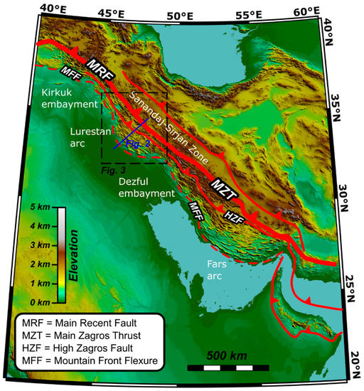
Figure 1.
Tectonic sketch map of the Zagros mountain belt.
The substantial strike-slip component associated with oblique plate convergence was accommodated by the composite lineament including the Main Recent Fault (MRF) and the Main Zagros Fault (MZT). This lineament separates the Arabian Plate to the SW from the Sanandaj-Sirjan Zone to the NE (Iran Block, Figure 2) [17,18,19,20,21]. The Sanandaj-Sirjan Zone was formed mainly by metamorphic rocks, by Jurassic to Early Eocene calc-alkaline magmatic rocks, and by the products of Middle Eocene gabbroic plutonism [1,22,23,24]. SW of the MRF-MZT composite lineament, the typical succession of the Arabian margin (Upper Triassic–Quaternary), largely folded and faulted due to the continental collision, sits on top of crystalline basement [25,26,27,28,29,30,31]. Here, the High Zagros Fault (HZF) separates the Simply Folded Belt to the SW from the Imbricate Zone to the NE (Figure 2). The latter zone includes the telescoped distal part of the original continental margin of the Arabian Plate (e.g., [31]). The mountain chain is bounded to the SW by the morphotectonic feature known as Mountain Front Flexure (MFF). This represents the topographic evidence of the crustal ramp of the major thrust fault of the study area, which we term here Main Frontal Thrust (MFT). The MFT is a blind crustal fault forming an upper flat at the basement-cover interface SW of the MFF (Figure 2) [7,13,17,26,32,33]. Recent geodetic measurements show that the northward relative motion of the Arabian Plate is still active today and occurs at ca. 20 mm yr−1 with respect to fixed Eurasia [8]. The MFT represents the main thrust in the outer part of the orogen and it is marked by intense seismic activity occurring at depths between 10 and 20 km [34], including the main seismic event (Mw = 7.3) of 12 November 2017 [13].
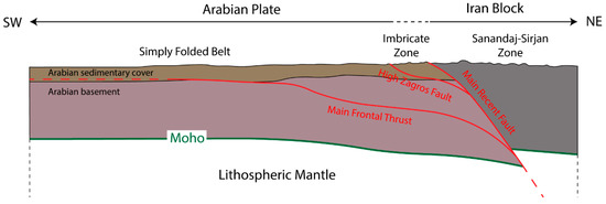
Figure 2.
Representative cross-section showing the main tectonic features of the Lurestan arc, which sketch map is shown in Figure 3. The thickness of the Arabian sedimentary cover and Arabian basement are defined in Section 3.2. The Moho discontinuity used for the analytical procedure is 3-D represented in Figure 4 and Figure 5.
3. Methods
In order to model the thermal structure of the Lurestan region of the Zagros thrust belt, a 3-D geological model was built for the area, shown in Figure 3. Using an analytical procedure, we calculated a geotherm for a series of vertical lines (pseudo-wells, shown in Figure 3). The resulting geotherms were then interpolated, producing a series of 3-D isotherms.
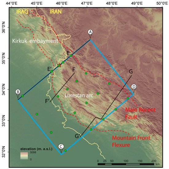
Figure 3.
Sketch map of the Lurestan arc. The yellow line represents the political boundary between Iraq and Iran. The blue rectangle is the area of the 3-D geological model shown in Figure 4, having vertexes A, B, C, and D. Black lines show the traces of published geological sections: (1) A - B by Basilici et al. [12], (2) E - E’ by Tavani et al. [13], (3) F-F’ by Tavani et al. [14], and (4) G-G’ by Vergés et al. [4]. Red, dashed lines are the traces of faults included in the geological 3-D model. Green points show location of the pseudo-wells used to implement the analytical procedure. Red star is the epicentral position of the main seismic event of 12 November 2017 (Mw = 7.3) [13].
3.1. The 3-D Geological Model
The 3-D geological model (Figure 4a) was implemented based on of the geological sections by Basilici et al. [12], Tavani et al. [13], Tavani et al. [14], and Vergès et al. [4], located in Figure 3. It results in a volume of 6,144,000 (320 × 240 × 80) km3 of rock. The topography was integrated in the model using a 30-m resolution ASTER GDEM. The resulting volume was divided into three different parts, assumed as homogeneous taking into account the resolution of thermal models at the crustal scale (e.g., [12]): (1) Arabian sedimentary cover, (2) Arabian basement, and (3) Iran block (or Sanandaj–Sirjan zone). The geological model (Figure 4b) took into account the MRF and the MFT, while minor faults were not included because of their negligible effect on temperature variations at the crustal scale. The Moho discontinuity was included in the model using the Moho depth calculated by Jiménez-Munt et al. [15] (Figure 4c).
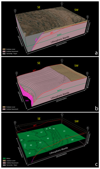
Figure 4.
The 3-D geological model. (a) Complete 3-D model of 6,144,000 (320 × 240 × 80) km3 of rock volume, based on geological sections by Basilici et al. [12], Tavani et al. [13], Tavani et al. [14], and Vergès et al. [4]. Topography is from a 30-m resolution ASTER GDEM. The model shows MRF (in purple), MFT (in red), and Moho (in green) in section. (b) MFT (red line) footwall topography, including deep sector beneath the branch line with the MRF (in purple). (c) Moho contours based on Jiménez-Munt et al. [15], with Moho depth in km (white numbers). In order to provide a better view of MRF and MFT geometry, the lithospheric mantle is not shown as a different block beneath the Moho discontinuity.
3.2. Constraints and Assumptions
The heat sources considered in the computation of the thermal structure were: (1) The heat rising from the mantle and (2) the radiogenic heat due to the presence of radioactive elements in the crust [35]. In thrust belts such as the Zagros, a further heat source is represented by frictional heating associated with thrust faulting. In the calculation of this latter heat source the shear stress was considered, which was obtained by Sibson’s [36] formulation for favorable oriented thrust faults at the chosen depths under hydrostatic pore-fluid conditions with a fixed friction coefficient.
To perform temperature calculations for the study area, we considered a series of pseudo-wells (located in Figure 3 and Figure 5).
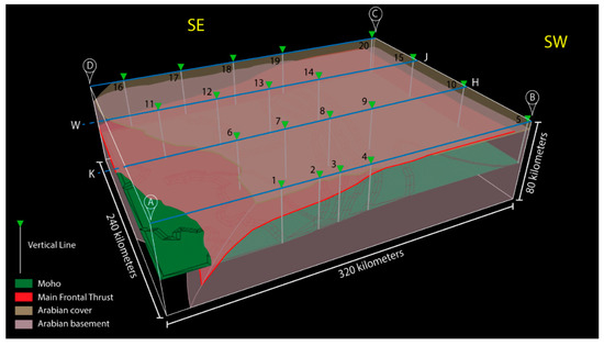
Figure 5.
The 3-D geological model with the location of pseudo-wells (grey vertical lines numbered 1 to 20) and section traces (blue lines, AB, KH, WJ, DC) used to perform the analytical procedure.
Input parameters included data on heat sources and geologically derived constraints (thrust depth, lithology) based on Tavani et al. [13]. A basal heat flow coming from the mantle was assumed, corresponding to a shield-type heat flow at the Moho [37]. For each pseudo-well (Figure 6) we considered the following parameters and assumptions:
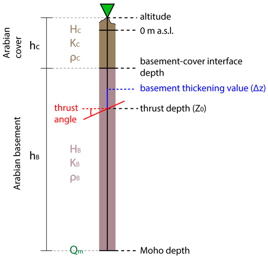
Figure 6.
Schematic representation of the different components included in the analytical geotherm calculation along one of the pseudo-wells of Figure 5. and are heat production rates for sedimentary cover and basement, respectively; is heat flux at Moho; and are thermal conductivity for the sedimentary cover and basement, respectively; ρc and ρb are density of the sedimentary cover and basement, respectively.
- (1)
- Altitude. We took into account the topography using the 30-m resolution ASTER GDEM.
- (2)
- Thickness of the Arabian cover (). We considered a variable thickness of the sedimentary cover based on the 3-D geological model (Figure 4), taking into account present-day topography (the model did not take into account erosion). The density of the Arabian cover was fixed to ρc = 2.55 × 10 3 [38].
- (3)
- Thickness of the Arabian basement (). We considered a variable thickness of the basement based on the depth of the Moho discontinuity calculated by Jiménez-Munt et al. [15]. The density of the basement was fixed to ρb = 2.80 × 10 3 [38].
- (4)
- Thrust depth and angle. The pseudo-wells crossed the MFT at different depths with a certain angle.
- (5)
- Amount of basement offset by the MFT (Δz). Taking into account the reconstructed geometry of the Arabian margin by Le Garzic et al. [39], we considered a total shortening of 20 km in the range of 20–10 Ma. The resulting slip rate () was in the range of 1–2 mm yr−1, and, therefore, we used an average value of 1.5 mm yr−1 [12]. The resulting basement thickening was in the range of 3.5–5.8 km. The friction coefficient (μ) was fixed to 0.6, according to Byerlee [40,41].
- (6)
- Constant heat production rate for the sedimentary cover () = 1.0 µW/m3 [11].
- (7)
- Constant heat production rate for the basement () = 0.4 µW/m3 [11].
- (8)
- Thermal conductivity for the sedimentary cover () = 2.0 Wm−1K−1 [11].
- (9)
- Thermal conductivity for the basement () = 2.2 Wm−1K−1 [11].
- (10)
- Heat flux at the Moho () = 20 mW/m2 [12,37].
3.3. Analytical Procedure
To obtain the geotherms we separated the calculation into two parts, one for the sedimentary cover () and the other for the basement (), with .
Basement thrusting, besides generating a new source of heat due to friction along the fault, produces a perturbation in the propagation of the mantle heat and an increase in radiogenic heat from the basement. Therefore, the basement temperature depends on the frictional heat (σv) and by the new equilibrium states reached both for the mantle heat () considered as constant and for crustal radiogenic heat ().
For the sedimentary cover, we considered the related radiogenic heat () and added the three perturbed conductive states due to: (1) The increase in radiogenic heat from the basement, (2) the perturbation of the mantle heat transfer, and (3) the frictional heat. Furthermore, we calculated the new perturbed states as a function of time based on the analytical equations by Molnar et al. [35], appropriately modified for overthrusting within a layered lithosphere [12,42].
Finally, the temperatures for the two, basement and sedimentary cover, layers can be obtained by the following equations:
where are not depth-dependent terms, with . Furthermore, each time-dependent term has the following generic expression:
with (Table 1)
where is the final temperature of the new state of equilibrium (, and and are the respective temperatures calculated at the top of the basement. In particular, , the only not-time-dependent term, is the temperature due to the radiogenic heat in the sedimentary cover, while is the temperature due to the propagation of the radiogenic heat in the lower (i.e., basement) layer considering the heat production due to overthrusting, is the temperature associated with the perturbed radiogenic heat in the basement, and and are the temperatures associated with the new perturbed state of the mantle and of the new heat source due to overthrusting.

Table 1.
Terms of the equations used for the analytical procedure.
To calculate the isotherms along the considered sections (AB, KH, WJ, and DC of Figure 5) we interpolated model data by a second-order power-law polynomial equation, obtaining the best-fit analytical curves approximating the geothermal values.
4. Results
Using the analytical procedure described in the previous paragraph, we calculated the geotherm for each pseudo-well shown in Figure 5. The result was a series of 20 geotherms, shown in Figure 6.
The geotherms relative to pseudo-wells 5, 10, 15, and 20 (yellow lines in Figure 7) showed a constant increment of temperature with depth due to the absence of basement offset by the MFT. On the other hand, all other pseudo-wells showed an increase of temperature variation with depth in correspondence to the MFT. In particular, the different trend of these geotherms depended on both the basement thickness modified by thrusting () and on the thrust depth. A weaker temperature increase occurred for the geotherms of pseudo-wells 4, 9, 14, and 19 (green lines in Figure 7), where the thrust was shallower and implied a smaller amount (3.5 km) of basement offset. All other geotherms showed higher temperature variations due to larger basement offsets ( in the range of 5.3–5.8 km) associated with thrusting occurring at progressively greater depths (from 18 to 36 km) moving towards the hinterland (i.e., from SW to NE).
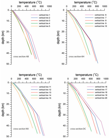
The sensitivity of this type of analytical procedure was checked by Megna et al. [43]. A variation of about 10% of thrust depth or slip rate produced a change of frictional heat that modified the final temperature by values never exceeding 2%.
In order to provide an effective overview of the temperature trend along each cross section (AB, KH, WJ, and DC of Figure 5), we interpolated the temperature data from 50 °C to 500 °C using a 50 °C step. The isotherms obtained by interpolating the data using a second-order power-law polynomial equation consisted of best-fit analytical curves with an rms (root mean square) error comprised between 0.6 and 3.75 (for the 100 °C and 500 °C isotherms, respectively).
The isotherms shown in Figure 8 (where a temperature step of 100 °C was used to allow a better visualization) define a general trend of increasing temperature moving from the foreland to the hinterland (i.e., from SW to NE) of the chain along each of the four cross-sections. Only the isotherm pattern along cross-section AB defined an upward curvature, thus confirming the previous 2-D study of Basilici et al. [12]. The isotherm pattern along cross-sections HK and JW show a gentle downward curvature, while more straight, SW-ward dipping isotherms characterize cross-section CD.
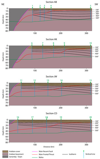
Figure 8.
Isotherms for the 100-500 °C temperature range (100 °C steps) calculated using a second-order power-law polynomial interpolation for cross-sections AB, KH, WJ, and DC (located in Figure 5).
5. Discussion
Based on the analytical results, isothermal surfaces were constructed using the minimum curvature spline interpolation technique. This allowed us to produce a series of maps for the 100 °C to 500 °C isotherms (Figure 9), as well as a 3-D model of the thermal structure of the Lurestan arc subsurface (Figure 10). A comparison of the latter with the thermal structure obtained by second-order power-law polynomial interpolation (Figure 11) shows a good fit between the two methods, thus confirming the consistency and robustness of the thermal structure depicted in Figure 10.
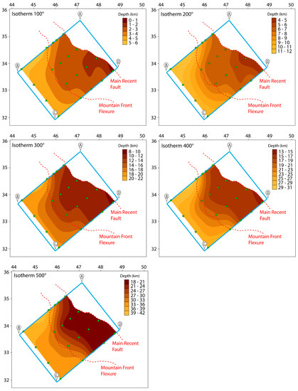
Figure 9.
Isotherm depth contour maps obtained by spline interpolation for the 100–500 °C temperature range (green dots are pseudo-wells used for geotherm calculation).
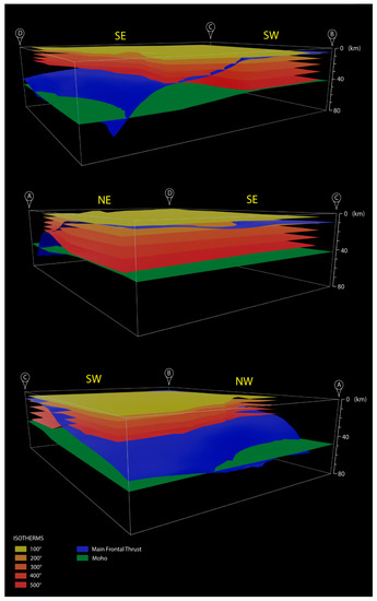
Figure 10.
Three different views of the 3-D thermal model obtained for the study crustal volume of the Lurestan arc. The model shows isotherms obtained with spline interpolation for the 100–500 °C temperature range (100 °C steps), together with the MFT and the Moho discontinuity, this latter obtained from Jiménez-Munt et al. [15].
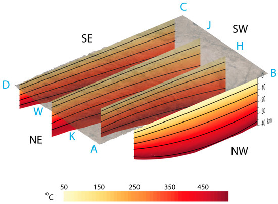
Figure 11.
Thermal structure of the Lurestan arc as defined by isotherms calculated using a second-order power-law polynomial interpolation along cross-sections AB, KH, WJ, and DC (located in Figure 5, black lines are 100, 200, 300, 400, and 500°C isotherms). Surface topography is from the 30-m resolution ASTER GDEM.
The isotherm depth contour maps of Figure 8 are characterized by a general SW-ward deepening of the isotherms, which clearly outline a higher temperature axial zone of the mountain belt and a “colder” outer zone including the foothills of the Simply Folded Belt and the adjacent foreland. The NE-ward temperature increment was mainly due to the crustal thickening associated with basement-involved faulting, as the NE dipping MFT produces a progressively increasing amount of basement offset by the fault (). The SW-ward deepening of the isotherms involved depth changes in the range of ca. 7 km to ca. 20 km for the 100 °C and 500 °C, respectively. The resulting thermal structure tended to mimic the general arc-shaped geometry of the mountain belt, as readily observable by comparing the isotherm depth contours with the trace of the MFF in the maps of Figure 9. As a matter of fact, the junction between the Lurestan arc (forming a salient of the Zagros fold and thrust belt) and the Kirkuk embayment (representing a recess) to the NW was clearly reflected by the crustal thermal structure observed in map view (Figure 9). The thermal structure shows a clear correlation with the geometry of the main thrust fault of the region, i.e., the MFT. According to Tavani et al. [14], the MFT developed in the necking domain of the Jurassic rift system ahead of an array of inverted Jurassic extensional faults, the related structural architecture resembling that of a crustal-scale footwall shortcut. As the main crustal ramp of the MFT underlies at depth the MFF, the sinusoidal shape of the latter in the Lurestan region would derive from the re-use of the originally segmented, inverted Jurassic rift system [14]. Despite this long-lived paleo-tectonic control and the fundamental role of structural inheritance, the development of the MFF, and thus the activity of the underlying thrust (MFT) controlling it, are recent processes. These are dated to ca. 3 Ma based on stratigraphic information [44], and to ca. 5 Ma based on low-temperature thermochronology data [7]. According to the latter studies, the major morphotectonic feature constituting the MFF developed during the Pliocene by basement-involved thrusting as deformation migrated downward at deeper crustal levels. Therefore, late-stage, crustal ramp-dominated thrusting [45] not only led to the development of a prominent geomorphological boundary between the high Zagros Mountains and the low foothills to the SW [17,32,33] but also appears to have exerted a major control on the thermal structure of the Lurestan salient.
The first-order, general pattern of foreland-ward deepening of the isotherms was rendered more articulated by along-strike variations, mainly consisting of a SE-ward climbing of the isotherms (Figure 9). Also, this along-strike, SE-ward temperature increase was essentially controlled by the 3-D geometry of the MFT, which is characterized by a low-angle crustal ramp in its SE portion, changing to a steep ramp rapidly reaching lower crustal depths to the NW (Figure 10). This is essentially because the gently dipping MFT segment produced a larger basement offset in the SE sector, where it joins the MRF along a branch line located within crustal depths (Figure 4 and Figure 10). This larger basement offset resulted in a more marked temperature increase and related shallower isotherms in the SE sector of the Lurestan arc (Figure 9). The along-strike variation in the thermal structure is readily observable in Figure 11. There, the widely spaced isotherm pattern of the NW “colder” edge of the model (i.e., at the junction with the Kirkuk embayment) gives way to a pattern characterized by progressively more densely spaced isotherms, which become closer to each other moving to the SE portion of the Lurestan arc. As a result, the easternmost sector of the study area represents a zone of relatively high geothermal gradient, particularly concerning temperatures <300 °C in the shallower part of the upper crust (Figure 9). This could have interesting implications in terms of geothermal energy potential in the region.
6. Conclusions
This study provides the first 3-D model of the thermal structure of the Lurestan arc of the Zagros thrust belt. Our results emphasize the major role played by a crustal thrust fault (i.e., the MFT) in controlling the thermal setting of the region. This is testified by a very good correlation between high temperature gradients in the crust and the amount of basement offset by the MFT. Besides a general temperature increase towards the hinterland, manifested by shallower and more densely spaced isotherms moving to the NE, there is also a marked along-strike variation associated with a lateral transition from a gently to a moderately dipping crustal ramp of the MFT. This results in a zone of relatively high geothermal gradient in the easternmost part of the study area. The marked effect of recent (i.e., Pliocene) thick-skinned inversion [14] and associated basement thrusting in perturbing the thermal structure, particularly at upper crustal levels, represents an interesting outcome to be taken into account in future geodynamic studies, as well as in geothermal/hydrocarbon exploration in the Lurestan region. It may also have important implications for active tectonic studies and seismotectonic modelling in an area recently affected by a Mw > 7 earthquake.
Author Contributions
Conceptualization, M.B., A.M., S.S., S.M. and S.T.; methodology, M.B., A.M., S.S., S.M. and S.T.; software, A.M. and M.B.; validation, M.B., A.M., S.S., S.M. and S.T.; formal analysis, M.B., A.M. and S.S.; investigation, S.T., S.M., M.B., A.M. and S.S.; resources, A.M. and S.S.; data curation, A.M., S.S., S.M. and S.T.; writing—Original draft preparation, M.B.; writing—Review and editing, S.M.; visualization, M.B.; supervision, S.S., S.M. and S.T.; project administration, S.S.; funding acquisition, S.S. All authors have read and agreed to the published version of the manuscript.
Funding
This research received no external funding.
Acknowledgments
The authors are grateful to the editor for his helpful support in organizing the manuscript. We thank two anonymous reviewers for their useful comments and suggestions.
Conflicts of Interest
The authors declare no conflict of interest.
References
- Alavi, M. Tectonics of the Zagros orogenic belt of Iran: New data and interpretations. Tectonophysics 1994, 229, 211–238. [Google Scholar] [CrossRef]
- Golonka, J. Plate tectonic evolution of the southern margin of Eurasia in the Mesozoic and Cenozoic. Tectonophysics 2004, 381, 235–273. [Google Scholar] [CrossRef]
- Agard, P.; Omrani, J.; Jolivet, L.; Whitechurch, H.; Vrielynck, B.; Spakman, W.; Monié, P.; Meyer, B.; Wortel, R. Zagros orogeny: A subduction-dominated process. Geol. Mag. 2011, 148, 692–725. [Google Scholar] [CrossRef]
- Vergés, J.; Saura, E.; Casciello, E.; Fernàndez, M.; Villaseñor, A.; Jiménez-Munt, I.; García-Castellanos, D. Crustal-scale cross-sections across the NW Zagros belt: Implications for the Arabian margin reconstruction. Geol. Mag. 2011, 148, 739–761. [Google Scholar] [CrossRef]
- Csontos, L.; Sasvári, Á.; Pocsai, T.; Kósa, L.; Salae, A.T.; Ali, A. Structural evolution of the northwestern Zagros, Kurdistan Region, Iraq: Implications on oil migration. GeoArabia 2012, 17, 81–116. [Google Scholar]
- Mouthereau, F.; Lacombe, O.; Vergés, J. Building the Zagros collisional orogen: Timing, strain distribution and the dynamics of Arabia/Eurasia plate convergence. Tectonophysics 2012, 532, 27–60. [Google Scholar] [CrossRef]
- Koshnaw, R.I.; Horton, B.K.; Stockli, D.F.; Barber, D.; Tamar-Agha, M.; Kendall, J.J. Neogene shortening and exhumation of the Zagros fold-thrust belt and foreland basin in the Kurdistan region of northern Iraq. Tectonophysics 2017, 694, 332–355. [Google Scholar] [CrossRef]
- Vernant, P.; Nilforoushan, F.; Hatzfeld, D.; Abassi, M.; Vigny, C.; Masson, F.; Nankali, H.; Martinod, J.; Ashtiani, A.; Bayer, R.; et al. Contemporary Crustal Deformation and Plate Kinematics in Middle East constrained by GPS Measurements in Iran and North Oman. Geophys. J. Int. 2004, 157, 381–398. [Google Scholar] [CrossRef]
- USGS.gov|Science for a Changing World. Available online: https://www.usgs.gov/ (accessed on 22 March 2020).
- Vernant, P.; Chéry, J. Mechanical modelling of oblique convergence in the Zagros, Iran. Geophys. J. Int. 2006, 165, 991–1002. [Google Scholar] [CrossRef]
- Tunini, L.; Jiménez-Munt, I.; Fernàndez, M.; Vergés, J.; Villaseñor, A. Lithospheric mantle heterogeneities beneath the Zagros Mountains and the Iranian Plateau: A petrological-geophysical study. Geophys. J. Int. 2015, 200, 596–614. [Google Scholar] [CrossRef]
- Basilici, M.; Mazzoli, S.; Megna, A.; Santini, S.; Tavani, S. Geothermal Model of the Shallow Crustal Structure across the “Mountain Front Fault” in Western Lurestan, Zagros Thrust Belt, Iran. Geosciences 2019, 9, 301. [Google Scholar] [CrossRef]
- Tavani, S.; Parente, M.; Puzone, F.; Corradetti, A.; Gharabeigli, G.; Valinejad, M.; Morsalnejad, D.; Mazzoli, S. The seismogenic fault system of the 2017 Mw 7.3 Iran-Iraq earthquake: Constraints from surface and subsurface data, cross-section balancing, and restoration. Solid Earth 2018, 9, 821–831. [Google Scholar] [CrossRef]
- Tavani, S.; Camanni, G.; Nappo, M.; Snidero, M.; Ascione, A.; Valente, E.; Gharabeigli, G.; Morsalnejad, D.; Mazzoli, S. The Mountain Front Flexure in the Lurestan region of the Zagros belt: Crustal architecture and role of structural inheritances. J. Struct. Geol. 2020, 135, 104022. [Google Scholar] [CrossRef]
- Jiménez-Munt, I.; Fernàndez, M.; Saura, E.; Vergés, J.; Garcia-Castellanos, D. 3-D lithospheric structure and regional/residual Bouguer anomalies in the Arabia–Eurasia collision (Iran). Geophys. J. Int. 2012, 190, 1311–1324. [Google Scholar] [CrossRef]
- Tavani, S.; Corradetti, A.; Sabbatino, M.; Morsalnejad, D.; Mazzoli, S. The Meso-Cenozoic fracture pattern of the Lurestan region, Iran: The role of rifting, convergence, and differential compaction in the development of pre-orogenic oblique fractures in the Zagros Belt. Tectonophysics 2018, 749, 104–119. [Google Scholar] [CrossRef]
- Berberian, M. Master “blind” thrust faults hidden under the Zagros folds: Active basement tectonics and surface morphotectonics. Tectonophysics 1995, 241, 193–224. [Google Scholar] [CrossRef]
- Talebian, M.; Jackson, J. Offset on the Main Recent Fault of NW Iran and implications for the late Cenozoic tectonics of the Arabia–Eurasia collision zone. Geophys. J. Int. 2002, 157, 381–398. [Google Scholar] [CrossRef]
- Blanc, E.J.-P.; Allen, M.B.; Inger, S.; Hassani, H. Structural styles in the Zagros Simple Folded Zone, Iran. J. Geol. Soc. 2003, 160, 401–412. [Google Scholar] [CrossRef]
- Allen, M.; Jackson, J.; Walker, R. Late Cenozoic reorganization of the Arabia-Eurasia collision and the comparison of short-term deformation rates. Tectonics 2004, 23, TC2008. [Google Scholar] [CrossRef]
- Authemayou, C.; Chardon, D.; Bellier, O.; Malekzadeh, Z.; Shabanian, E.; Abbassi, M.R. Late Cenozoic partitioning of oblique plate convergence in the Zagros fold-and-thrust belt (Iran). Tectonics 2006, 25, TC3002. [Google Scholar] [CrossRef]
- Berberian, F.; Berberian, M. Tectono-Plutonic Episodes in Iran. In Zagros-Hindu Kush-Himalaya Geodynamic Evolution, Geodynamics Series; Gupta, H.K., Delany, F.M., Eds.; American Geophysical Union: Washington, DC, USA, 1981; Volume 3, pp. 5–32. [Google Scholar]
- Leterrier, J. Mineralogical, Geochemical and isotopic evolution of two Miocene mafic intrusions from the Zagros (Iran). Lithos 1985, 18, 311–329. [Google Scholar] [CrossRef]
- Baharifar, A.; Moinevaziri, H.; Bellon, H.; Pique, A. The crystalline complexes of Hamadan (Sanandaj-Sirjan zone, western Iran): Metasedimentary Mesozoic sequences affected by Late Cretaceous tectono-metamorphic and plutonic events. C. R. Geosci. 2004, 336, 257–282. [Google Scholar] [CrossRef]
- Colman-Saad, S.P. Fold development in Zagros simply folded belt, southwest Iran. Am. Assoc. Pet. Geol. Bull. 1978, 62, 984–1003. [Google Scholar] [CrossRef]
- Sepeher, M.; Cosgrove, J.W. Structural framework of the Zagros Fold–Thrust Belt, Iran. Mar. Pet. Geol. 2004, 21, 829–843. [Google Scholar] [CrossRef]
- Jassim, S.Z.; Goff, J.G. Geology of Iraq, 1st ed.; Prague and Moravian Museum: Brno, Czech Republic, 2006. [Google Scholar]
- Rudkiewicz, J.L.; Sherkati, S.; Letouzey, J. Evolution of Maturity in Northern Fars and in the Izeh Zone (Iranian Zagros) and Link with Hydrocarbon Prospectivity. In Thrust Belts and Foreland Basins; Lacombe, O., Roure, F., Lavé, J., Vergés, J., Eds.; Frontiers in Earth Sciences; Springer: Berlin/Heidelberg, Germany, 2007. [Google Scholar]
- Casciello, E.; Vergés, J.; Saura, E.; Casini, G.; Fernàndez, N.; Blanc, E.J.P.; Homke, S.; Hunt, D. Fold patterns and multilayer rheology of the Lurestan Province, Zagros Simply Folded Belt (Iran). J. Geol. Soc. Lond. 2009, 166, 947–959. [Google Scholar] [CrossRef]
- Law, A.; Munn, D.; Symms, A.; Wilson, D.; Hattingh, S.; Boblecki, R.; Al Marei, K.; Chernik, P.; Parry, D.; Ho, J. Competent Person’s Report on Certain Petroleum Interests of Gulf Keystone Petroleum and Its Subsidiaries in Kurdistan, Iraq; ERC Equipoise Ltd: Croydon, UK, 2014. [Google Scholar]
- Tavani, S.; Parente, M.; Vitale, S.; Iannace, A.; Corradetti, A.; Bottini, C.; Morsalnejad, D.; Mazzoli, S. Early Jurassic Rifting of the Arabian Passive Continental Margin of the Neo-Tethys. Field Evidence from the Lurestan Region of the Zagros Fold-and-Thrust Belt, Iran. Tectonics 2018, 37, 2586–2607. [Google Scholar] [CrossRef]
- Falcon, N.L. Major earth-flexuring in the Zagros Mountains of south-west Iran. Q. J. Geol. Soc. Lond. 1961, 117, 367–376. [Google Scholar] [CrossRef]
- Emami, H.; Vergès, J.; Nalpas, T.; Gillespie, P.; Sharp, I.; Karpuz, R.; Blanc, E.J.P.; Goodarzi, M.G.H. Structure of the Mountain Front Flexure along the Anaran anticline in the Pusht-e Kuh Arc (NW Zagros, Iran): Insights from sand box models. Geol. Soc. Lond. Spec. Publ. 2010, 330, 155–178. [Google Scholar] [CrossRef]
- Engdahl, E.R.; Jackson, J.A.; Myers, S.C.; Bergman, E.A.; Priestley, K. Relocation and assessment of seismicity in the Iran region. Geophys. J. Int. 2006, 167, 761–778. [Google Scholar] [CrossRef]
- Molnar, P.; Chen, W.P.; Padovani, E. Calculated temperatures in overthrust terrains and possible combinations of heat sources responsible for the tertiary granites in the greater Himalaya. J. Geophys. Res. 1983, 88, 6415–6429. [Google Scholar] [CrossRef]
- Sibson, R.H. Frictional constraints on thrust, wrench and normal faults. Nature 1974, 249, 542–544. [Google Scholar] [CrossRef]
- Francois, T.; Burov, E.; Agard, P.; Meyer, B. Buildup of a dynamically supported orogenic plateau: Numerical modeling of the Zagros/Central Iran case study. Geochem. Geophys. Geosyst. 2014, 15, 2632–2654. [Google Scholar] [CrossRef]
- Teknik, V.; Ghods, A.; Thybo, H.; Artemieva, I.M. Crustal density structure of the northwestern Iranian Plateau. Can. J. Earth Sci. 2019, 56, 1347–1365. [Google Scholar] [CrossRef]
- Le Garzic, E.; Vergés, J.; Sapin, F.; Saura, E.; Meresse, F.; Ringenbach, J.C. Evolution of the NW Zagros Fold-and-Thrust Belt in Kurdistan Region of Iraq from balanced and restored crustal-scale sections and forward modeling. J. Struct. Geol. 2019, 124, 51–69. [Google Scholar] [CrossRef]
- Byerlee, J.D. Frictional characteristics of granite under high confining pressure. J. Geophys. Res. 1967, 72, 3639–3648. [Google Scholar] [CrossRef]
- Byerlee, J.D. Friction of rocks. J. PAGEOPH 1978, 116, 615. [Google Scholar] [CrossRef]
- Candela, S.; Mazzoli, S.; Megna, A.; Santini, S. Finite element modelling of stress field perturbations and interseismic crustal deformation in the Val d’Agri region, southern Apennines, Italy. Tectonophysics 2015, 657, 245–259. [Google Scholar] [CrossRef]
- Megna, A.; Candela, S.; Mazzoli, S.; Santini, S. An analytical model for the geotherm in the Basilicata oil fields area (southern Italy). Ital. J. Geosci. 2014, 133, 204–213. [Google Scholar] [CrossRef]
- Homke, S.; Verges, J.; Graces, M.; Emami, H.; Karpuz, R. Magnetostratigraphy of Miocene–Pliocene Zagros foreland deposits in the front of the Pushe Kush Arc, (Lurestan Province, Iran). Earth Planet. Sci. Lett. 2004, 225, 397–410. [Google Scholar] [CrossRef]
- Butler, R.W.H.; Mazzoli, S. Styles of continental contraction: A review and Introduction. In Styles of Continental Contraction; Mazzoli, S., Butler, R.W.H., Eds.; Geological Society of America: Boulder, CO, USA, 2006; Volume 414, pp. 1–10. [Google Scholar] [CrossRef]


© 2020 by the authors. Licensee MDPI, Basel, Switzerland. This article is an open access article distributed under the terms and conditions of the Creative Commons Attribution (CC BY) license (http://creativecommons.org/licenses/by/4.0/).