Abstract
Numerical models of geothermal doublet allows us to reduce the high risk associated with the selection of the most effective location of a production well. Furthermore, modeling is a suitable tool to verify possible changes in operational geothermal parameters, which guarantees liveliness of the system. An appropriate selection of software as well as the methodology used to generate numerical models significantly affects the quality of the obtained results. In this paper, the authors discuss the influence of such parameters as grid density and distance between wells on the efficiency of geothermal heating plant. The last stage of the analysis was connected with estimation of geothermal power potential for a hypothetical geothermal doublet. Numerical simulations were carried out using the TOUGH2 code, which applies the finite-difference method. The research was conducted in the Szczecin Trough area (NW Poland), based on archival data from Choszczno IG-1 well. The results demonstrated that in the studied case of the Choszczno region, the changes in the distance of boreholes can have a visible influence on obtained results; however the grid density of the numerical model did not achieve a significant impact on it. The results show the significant importance of numerical modeling aimed at increasing the efficiency of a potential geothermal heating plant.
1. Introduction
Geothermal waters and energy utilization have a beneficial impact that improves the living conditions in any region where existing geothermal resources enable its effective use [1,2]. It is the kind of renewable energy whose resources are available regardless of weather conditions throughout the year and around all day. However, the basic condition for successful investment is the existence of appropriate hydrogeothermal conditions at the place of its implementation [3,4,5]. In Poland, low-temperature geothermal resources occur in many parts of the country. Research carried out so far confirms that the main resources of geothermal waters in the Polish Lowlands are accumulated in the Mesozoic groundwater horizons, mostly in Lower Jurassic and Lower Cretaceous aquifers. This kind of resources should be, first of all, used for heating purposes [6,7,8].
High capital expenditures and very low running costs are a characteristic feature of geothermal investments. An important element is the fact that the majority of costs transferred during the construction of the installation are independent of the amount of heat extracted from the generated geothermal water. To ensure low unit costs of heat extraction, it is important to effectively design the geothermal installation [9,10,11,12,13]. The use of numerical modeling for this purpose brings many measurable benefits. Recently, modeling plays a crucial role even at the early stages of planning and designing geothermal investments [14,15,16]. The numerical models enable us to recognize both the geological structure of rock formations and the processes which operate within them [17,18,19,20,21]. Many interesting aspects of heat transfer and fluid flow in geothermal applications can be found in numerous publications [22,23,24,25,26,27]. There have been many attempts to analyze heterogeneous porous materials especially when it correlates with physical parameters [28,29]. Possibilities of modelling this kind systems using basic law for porous materials can be considered in few approaches: (1) extension of the Darcy equation to the Brinkmann–Darcy–Forchheimer equation [30]; (2) consideration of slip flow and thermal transpiration in media with high surface density [31,32,33]; (3) a model from which one can describe the Klinkenberg effect [34]. Numerical methods can also be applied to the prediction of possible unwanted processes accompanying the exploitation of groundwater, like the clogging of wells [35], corrosion of casings and surface installations [36], as well as mass exchange within the rock formations, which is crucial for prognosing the migration of contaminants [37].
In the case of mass and heat transfer, three methods are applied in numerical modeling: finite element method, finite volume method, and finite difference method [38,39,40]. These three methods are widely used by specialized simulators. Such tools facilitate the computations and enable us to determine the potential of the explored area and/or to select appropriate operational parameters of given geothermal installation in order to ensure its long life and failureless running [41,42,43]. Available numerical simulators for geothermal applications are mainly based on two computational methods: the finite element method (FEM) and the finite difference method (FDM). These methods differ from each other mainly by discretization methods. The FDM method seems to be more widely used in the simulation related to the flow of reservoir medium, probably due to the simplicity of the construction of the regular computational grid and the solution procedures used. However, for complex model geometry it is necessary to use FEM, for more complicated regions. In this work the Integrated Finite Difference Method (IFDM) was used. IFDM combines the advantages of both methods (FEM and FDM) by the possibility of compaction grid density in places where obtaining a precise result is the most important, using a computational method based on the change of differential operators to differential ones [38,41,42,43].
Taking into account the high costs of drillings, a reasonable idea is to run a series of simulations before any critical investment decision is made. This may eliminate many mistakes resulting from unwary solutions accepted at the initial stages of investments and may also facilitate the selection of the most effective parameters of future installations, as e.g., pattern of wells (location and number), their spacing, and wellbore diameters. Numerical computations always procure errors resulting, among others, from simplistic assumptions we apply in the modeling. However, the credible models must provide quantitative and qualitative results which are in agreement with the nature of processes they describe. The errors unrelated to modeling methodology originate from, e.g., the quality (correctness) of geological, geophysical, hydrogeological, and other data acquired in an exploration area [44,45,46,47,48]. The modeling errors depend on the selected numerical method, i.e., on applied software, on the size of selected area of modeling (which cannot be either too small or too large—the latter unnecessarily extends the computation time), as well as on the selection of boundary conditions and mode of their input. Important is also the experience of staff members who run the simulations; precisely, how much they are capable of interpreting the results and evaluating their credibility. The crucial aspect of modeling is the proper selection of a calculation grid, which enables higher performance of the computation process depending on the studied case. Generally, higher density of calculation grid increases the accuracy of modeling, but on the other hand, it extends the time of computations. As long as this time increases from several to some tens of minutes, the grid densification does not cause problems. If, however, such an extension prolongs to some tens of hours (or even more), the computation time turns into a serious obstacle, which is the common case of more complicated models. For simple models, in which the succeeding rock layers are almost parallel, we can select quite a sparse calculation grid without declining the quality of modeling. The factor usually analyzed with the numerical modeling is the mutual influence of geothermal wells. Such modeling enables us to assess the distance between production and injection boreholes to extend the lifetime of the system but also to decrease the energy transfer loss and to reduce the costs of connection pipelines. Considering the above, TOUGH2 code was chosen for numerical analysis, which is described in numerous scientific publications [49,50,51,52,53].
The main aim of the study is to evaluate two parameters, namely, calculation grid density and distance between wells on the results of simulation carried out by using TOUGH2 code. Another objective is to determine the geothermal potential in the Szczecin Trough, based on the archival Choszczno IG-1 well. Numerical simulations are a common tool for geothermal investments especially in the initial stage of the design process, but also by improving the operating ones. The article proposes a methodology for the effective improvement of the simulation by selecting a computational grid density that will guarantee precise results while reducing simulation time. Attention was also paid to simulations related to the distance between production and injection wells that has an impact on the system’s work but also on investment costs. In addition, based on the derived real hydrogeological model of the Szczecin Trough area, a numerical analysis of geothermal utilization was carried out in order to assess the thermal power of the source and the amount of energy obtained during operation. The temperature and pressure of extracted and injected fluids into the reservoir was estimated for 50 years of system activity. The obtained results are essential for the development of a sustainable geothermal heating plant and constitute a unique case study for exploitation of similar geothermal resources.
The paper is organized as follows. Summaries of a geological background that focuses on Szczecin Trough (NW part of Poland) are presented in Section 2. The numerical model is given in Section 3. The exposition of the results of numerical simulation is shown in Section 4. A brief estimation of the thermal power is presented in Section 5. Discussion considering three important issues, namely: (1) the changes of grid density; (2) the impact of distance between the geothermal wells; (3) estimation of geothermal power potential for a hypothetical geothermal doublet, is demonstrated in Section 6. Concluding remarks are formulated in Section 7.
2. Geological Background
Numerical modeling was performed for the Choszczno Anticline located within the geological structure named the Szczecin Trough (NW part of Poland) (Figure 1). For modeling purposes, the Choszczno IG-1 well had been selected as a geothermal production well. The Choszczno IG-1 well is located in the vicinity of Szczecin town.
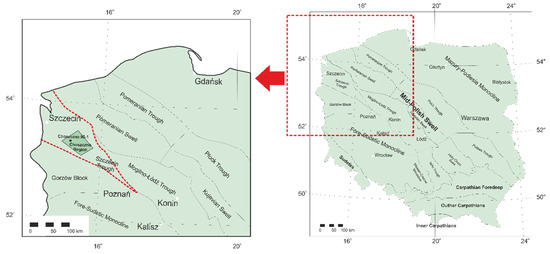
Figure 1.
Location of the study area on the background map of the main tectonic units of Poland on the sub-Cenozoic surface [54].
The lithostratigraphic profile of the Szczecin Through is built of partially eroded and folded Carboniferous-Devonian deposits covered with Rotliegend, Zechstein, and Mesozoic deposits. The most promising groundwater horizons occurs in the Lower Jurassic sandstones, mostly Hettangian and Sinemurian. Pliensbachian and Upper Toarcian deposits have less favorable reservoir parameters [20,21].
In the Choszczno area, the Lower Jurassic succession occurs at a depth interval from 1164.5 to 1468.0 m below sea level (bsl) and reaches a thickness of 303.5 m (Figure 2). Beneath the Lower Jurassic reservoir, the Upper Triassic clayey-sandy sediments occur. These are underlain by Middle Triassic (Muschelkalk) carbonates. Total thickness of Upper-Middle Triassic strata reaches 444.5 m (as revealed by data from the Pławno-1 well, see [55]). The Lower Jurassic succession is covered by Middle Jurassic sediments, 114.0 m thick, followed by Upper Jurassic, alternating sandstones and mudstones of thickness 53 m. The Jurassic formation is overlain by Cretaceous sediments, 842.8 m thick, followed by Tertiary (6 m thick) and Quaternary (148.7 m thick) stratum [56,57].
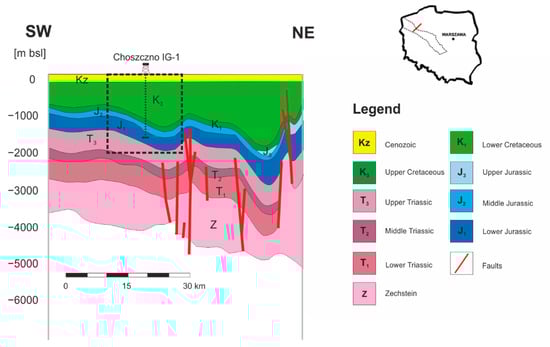
Figure 2.
Geological cross-section through Szczecin Trough according to [36], modified. The black rectangle shows the range of the numerical model for which simulations of the geothermal doublet were carried out.
In the Szczecin Trough, the density of heat flux to the Earth’s surface is the highest in Poland and varies from almost 70 to over 100 mW/m2. The minimal values (about 70–75 mW/m2) are recorded along the eastern margin of the trough, whereas the highest ones (over 90 mW/m2) occur in its southern part. In the Choszczno area, heat flux density is about 80–85 mW/m2 [58]. Such high flux corresponds to the pattern of subsurface temperatures, which vary from 50 °C in the top part to about 60 °C in the bottom part of the Lower Jurassic geothermal reservoir [20,21,59]. Such values correlate well with the temperature log recorded in the Choszczno IG-1 well from which both the geothermal step and geothermal gradient were calculated [60]. The geothermal step is 52.4 m/°C, hence, temperatures of the groundwaters at about 1390 m bsl reach 45.5 °C. Water mineralization is around 100–125 g/dm3, while the potential discharge of wells is about 200 m3/h [20,21].
The results of laboratory studies carried out at the Polish Geological Institute for samples from the Choszczno IG-1 well provided the mean values of effective porosity and density for particular stratigraphic units. The best reservoir properties were found in both the Upper and Lower Sinemurian sediments, for which the effective porosity exceeds 20% [61].
3. Numerical Methodology and Mathematical Model
The numerical model covered the area of 11.5 × 10.0 × 2.3 km (Figure 3). The geothermal doublet was based upon the archival information from the Choszczno IG-1 well, which was defined in the model as the production well. In this section a mathematical model of the whole system is presented also. Governing equations for fluids are strictly connected with the elementary balance of mass, momentum, and energy. However, the governing equation in solids is focused on the balance of energy. For porous rocks in the governing equations, porosity should be considered. In addition, the porosity of rocks, as follows: , is considered in governing equations. Typically, for each geological formation the values of rock porosity are the factors that take into account the amounts of fluid volume in respect to the whole volume of rocks formation . This paper uses the traditional system of equations for numerical modelling, namely [62,63]:
in which: is local derivative, means divergence, ; ; represents the relevant conserved variable vector. These variables (; ; ) are generated from the well-known equations: balance of mass (), the balance of momentum (—three equations), the balance of energy (). However, represents the density that can change in time and space . Indices and
refer to fluid and solid, respectively.
is velocity vector including
(versor in one direction defines by subscript ) and
(scalars magnitude of vector ); is the momentum density vector, represents pressure; is unit tensor,
means Kronecker’s delta. Additionally, diffusive momentum flux
takes into account laminar viscous stress flux.
is momentum sources which includes Darcy’s force acting as an extra source in the momentum balance equation. The total specific energy
consists specific kinetic energy and specific internal energy , where is specific heat capacity and is temperature. is the diffusive heat flux. Last but not the least, represent the energy sources in fluid and solid body, respectively. Measuring fluid mass flow rates in porous materials may help to predict the sum of effects of both the thermal transpiration and surface velocity slip. An additional bulk influence of viscous flow (Poiseuille’s type) is visible for the pores greater than 2–5 times the free length of molecules. In this specific case, the mass flow rate is the common effect of one bulk and two surface phenomena. Therefore, the resultant flow velocity of filtration is governed by the Poiseuille-Knudsen-Reynolds equation [64].
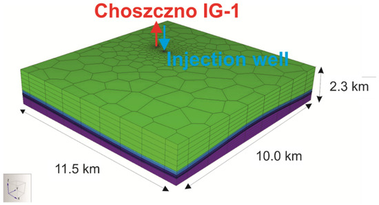
Figure 3.
Numerical model of Choszczno region.
Based on the integrated finite difference method (IFDM), the simulator discretizes both space and time. In the case of space, it is discretized to form basic differential equations. The TOUGH code has been continuously developed and successively validated for more than 35 years, as evidenced by the work initiated by Pruess [65,66,67,68] and subsequent numerous tests confirming its reliability based on benchmark experiments and multi-variant validation [69,70,71,72,73,74,75,76,77,78]. Therefore, the authors of this paper have based their work on previously conducted validations and focused only on model calibration based on available geological parameters.
Also, the issues concerning the generation of the discretization grid and its usefulness for modelling various physical phenomena have been developed in recent years, which is evidenced by a number of works [79,80,81,82]. Therefore, it was based on previous works on mesh for TOUGH2 code and prepared the grid as follows. The number of elements with defined volume is determined, as well as the method of connection between elements, enabling the creation of regular or irregular one-, two-, or three-dimensional interpolation meshes. Time discretization occurs by determining the number of simulation steps and can also apply to its total duration. Intervals for individual simulation steps were automatically selected by the simulator. Numerical simulations were conducted in PetraSim, which uses TOUGH code for the calculating process. Density of computational grid was changed by the maximum area near the wells located in the Choszczno Region, but without any changes in number of grid elements that equals 1616 elements.
At the first stage of the simulation, the hypothetical injection well was located about 1000 m from the production borehole. After implementation of both wells into the model, the polygonal calculation grid was superimposed, and calibration process was carried out again. The production well was designed at a depth of 1360 m. The injection borehole reached the depth of 1420 m. Both wells were designed at the level of Upper Synemurian Beds groundwater horizons, which guaranteed a closed groundwater circulation system within the Lower Jurassic geothermal reservoir. The yield of the geothermal doublet was planned as 120 m3/h and the lifetime of the installation was assumed as 50 years, at the temperature of injected water at the level of 25 °C.
The numerical model of the Choszczno region included 8 stratigraphic formations. For each geological formation the values of rock density, porosity, permeability, thermal conductivity, and specific heat value were defined individually as shown in Table 1. The values were introduced from well data [55], most of them were average values for subsequent stratigraphic formations. Values of thermal conductivity coefficient and specific heat were introduced with reference to lithological data [55].

Table 1.
Parameters defined for the model of Choszczno region [55].
The simulations were started from a conceptual model for which a regular calculation grid was implemented. Constant values of pressure and temperature were attributed to the top surface (in contact with the atmosphere) and the bottom surface, using the first type (Dirichlet) boundary condition. Then, the model was calibrated with the measured values. The results of calibration are shown in Figure 4. Due to the availability of the temperature curve from the Choszczno IG-1 well, the curve was used for the calibration process. During calibration, the permeability and thermal conductivity values were mainly changed. The results obtained during the calibration process were compared with the temperature curve from the Choszczno IG-1 well. Figure 4 shows the final calibration result which was considered sufficient for further analysis.
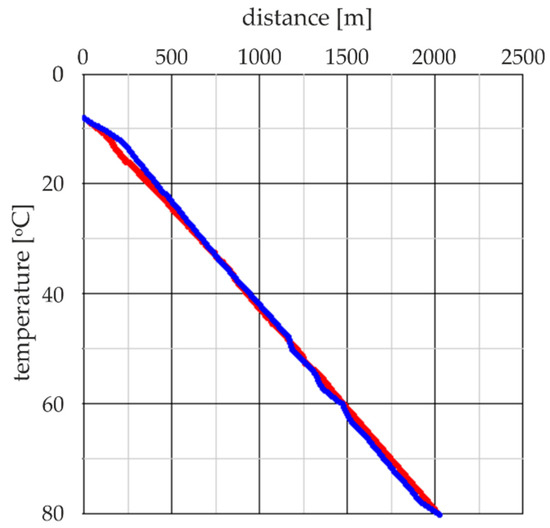
Figure 4.
Results of calibration of numerical model. Red line—the measured value for the Choszczno IG-1 well, blue line—the estimated value.
The obtained model was evaluated as a good representation of reality. Then, the regular grid was changed to a polygonal type, which allowed increasing density of the mesh near the boreholes. The calibration process was refined. Before starting numerical simulations, the model was re-calibrated to eliminate any errors related to the distribution of initial conditions in the newly defined model grid. The estimated results were compared once again with temperature from the Choszczno IG-1 well. The process was completed after receiving the best match. It should be mentioned that in the study [78], similar accuracies were obtained in the compatibility between the temperature distribution obtained experimentally and numerically. Additionally, the study [78] shows that the model is calibrated and achieves convergence between the measured and calculated pressure distribution. Therefore, it was assumed that a similar convergence would be obtained for pressure if only a pressure distribution for the Choszczno IG-1 borehole would be available.
In this article, the direct “optimization” method, consisting in the cyclical change of the input calculation parameters (according to the established scenario) in order to approximate more refined and higher resolution of the proposed cases, is presented. The evaluation process includes two goal functions. The first concerned issues related to the numerical modelling and included the choice of resolution—computational grid density. Dense grids improve the accuracy of the solution, but unfortunately their use extends the calculation time, which significantly affects the selection process. This is particularly important for direct “optimization” methods, which were used in the article to look for the extreme of the second objective function. The second objective function was to determine the smallest safe distance between the wells of the geothermal doublet. The measure of safety was analyzed by the time when breakthrough of the cold front between the injection and production well, was observed. The smallest distance for which no significant decrease in the temperature of the geothermal fluid was estimated, was considered as the most appropriate but addressable only for analyzed cases. Therefore, mathematically speaking, what has been proposed here is not a “global” optimization scheme, but it is an assessment of the effective variants leading to higher performance for the studied cases, using numerical analyses.
However, limitation of the distance between production and injection wells affects the costs of geothermal doublet by reducing the length of pipeline between wells [83] and therefore various types of optimization have been developed. Apart from the proposed direct "optimization" method, we also distinguish other techniques of searching for an optimal solution, among them: surrogate models [84], Bayesian functions examining the probability of occurrence of various conditions [85], optimizations taking into account the process economy [86], or discrete network modeling [87]. However, it is still important to take proper account of the quantity and quality of the energy produced, which has been described, among others, in the works: [88,89,90] in which the quality of the energy produced has been optimized. Another aspect is the optimization of the location of boreholes [91,92] and the deposit’s lifetime [93,94]. Recently, articles have been published which consider many different criteria of optimization and put different weightings on every standard due to different types of conditions [95,96,97].
4. Results of Numerical Simulation
At the first stage of the simulations, the results obtained for various polygonal grids were compared. The polygonal grid comprises a set of polygons (grid blocks) of various dimensions (Figure 5).
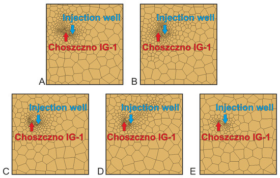
Figure 5.
Variants of calculation grid density calculation. Areas of grid blocks: A—1 m2, B—10 m2, C—100 m2, D—1000 m2, E—10,000 m2.
These blocks were densified around the wells, which provided more accurate results of modeling in the rock volume influenced by production-injection cycles. The impact of changes in the density of grid nodes clustered around the wells for values (Figure 5): 1 m2, 10 m2, 100 m2, 1000 m2, 10,000 m2, was analyzed.
Simulations were carried out for each grid density variant taking into account the following parameters: designed discharge of production well 120 m3/h, temperature of injected water 25 °C, 1000 m distance between wells and 50-year-long lifetime of the heating plant. As a result, changes in time of pressure and temperatures values in production and injection wells (Figure 6) were observed.
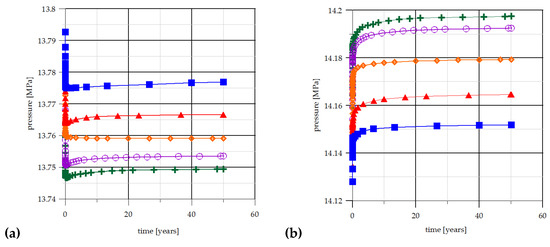
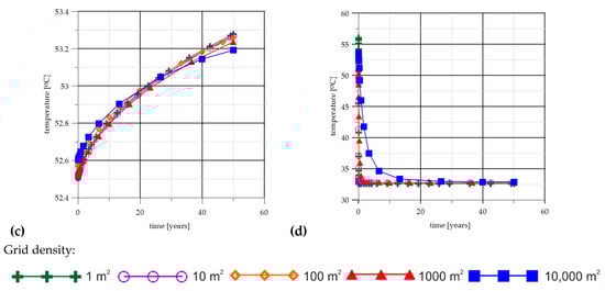
Figure 6.
Changes of the pressure (a) in production and (b) in injection well zones, and temperature (c) in production and (d) in injection well zones for various densities of grid calculation.
Based on results in Figure 6, it can be observed that for density from 1 to 100 m2 estimated values are similar. The most visible differences are visible for the density between 1000–10,000 m2. Furthermore, taking into consideration the simulation time, which increases with increasing density, for 1 m2 time is approximately 4 times longer than for 100 m2 density. For further calculations, the 100 m2 density was assumed as the most effective for the Choszczno region. Presented and preceding published [98] tests allowed to choose the numerical grid to ensure that further refinement insignificantly influence the temperatures and pressures variation in time. Since then, several simulations have been carried out, which affected the final density of the grid. Therefore, computational results for 100 m2 density can be treated as mesh independent.
At the second stage of the simulation, the distance between production and injection wells in ranges of: 3000, 2500, 2000, 1500, 1000, 500 m (Figure 7), was analyzed. Pressure in the production borehole zone changes from 13.749 MPa (for 3 000 m) to 13.762 MPa (for 500 m), while in the injection well pressure increased from 14.001 MPa (for 500 m) to 15.018 MPa (for 3000 m). The temperature of the injected water for a period of 50 years in the distance range of 1000 to 3000 m between wells is stable, only for the distance range of 500 m the temperature in production well zone drops up to 1.6 °C (Figure 7). The obtained results were compared with the results of other analyses carried out for the research area in recent years [20,21,36]. The results were also referred to the parameters of geothermal heating plants located in Stargard and Pyrzyce, in a short distance from the research area. In both cases it was confirmed that they are correct.
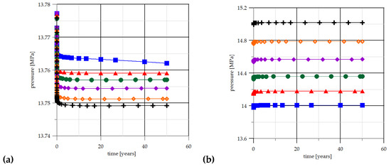
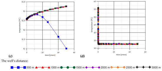
Figure 7.
Variants of spacing between wells (a) in production and (b) in injection well zones, and temperature in (c) production and (d) injection well zones for various well distance.
5. Thermal Power Estimations
Based on the results of numerical simulations, the thermal power for the geothermal doublet versus grid density (Figure 8) and versus distance between production and injection wells (Figure 9), were estimated. However, the wellhead temperature doesn’t differ very much from the influence on thermal power as to be noticeable. The thermal power of the geothermal doublet was calculated according to the formula:
where:
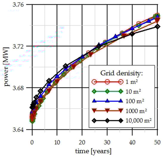
Figure 8.
Variation of thermal power vs. time as function of grid density.
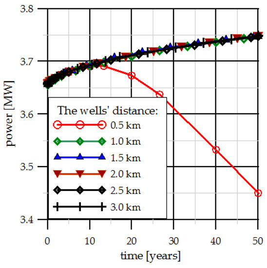
Figure 9.
Variation of average annual thermal power vs. time as function of distance between wells (grid density 100 m2).
- —thermal power of geothermal doublet (W),
- —brine outflow (m3/s),
- —brine specific heat (J/(kg K),
- —brine density (kg/m3),
- —brine temperature (°C),
- —assumed reference temperature (°C).
The brine outflow and reference temperature were assumed at 120 m3/h and 25 °C. Brine temperature was estimated by numerical modeling. Thermal properties of the brine and were estimated based on the [99] assumed salinity as 120 g/L and mean temperature between and at the level of approximal 40 °C. The rest of the data was determined on the basis of a commonly accepted methodology [13,100,101,102]. The brine density was estimated at 1090 kg/m3 and specific heat at 3.65 (kJ/(kg K)). For specific variability of thermal power, it was possible to determine the amount of energy produced in the analyzed time period (i.e., 50 years). The amount of thermal energy generated by the installation and coming from geothermal energy was determined by the relationship:
where:
- —thermal energy (J),
- —thermal power of geothermal doublet (W),
- —time (s).
Based on energy, it is possible to determine the average annual heat output of the installation over a 50-year period:
where:
- —annual average thermal power of geothermal doublet (W),
- —energy received during time period (J),
- —analysed time period (s).
In addition, based on energy received for 50 years (), it can be estimated the average amount of energy produced annually, as follows:
where:
- —average amount of energy produced annually (J),
- —energy received during time period (50 years) (J),
- —number of years.
The amount of average energy produced annually and average annual thermal power for the analyzed variants are listed in the Table 2. Figure 8 shows the results of numerical simulations of the thermal power for the geothermal doublet versus grid density in order to check mesh independence of resolution. However, the wellhead temperature does not differ very much in Figure 6., in which the influence on thermal power has been considered. In addition, Table 2 presents the average amount of energy produced annually (TJ/yr) and averaged power of the geothermal doublet to highlight that slight fluctuation of those parameters is observed.
Table 2.
Average amount of energy produced annually (TJ/yr) and averaged thermal power of the geothermal doublet—results in analyzed variants.
6. Discussion
Conducted simulations confirmed the possibilities of geothermal energy utilization in the Choszczno Region, which was indicated as a prospective area in terms of geothermal energy utilization [20,21,36]. Taking into account the results of grid density simulations (Figure 6), it is visible that 100 m2 density ensures sufficient precision. The differences of values for estimated parameters between 1 and 100 m2 density were not significant. The estimated pressure values for the production well zone vary in the range of 13.75–13.78 MPa, which gives changes up to 0.22%. In the case of the injection well, the observed changes are higher, in the range of 14.15–14.20 MPa, which gives a difference up to 0.35%. Pressure values in both cases stabilize between first and second year of exploitation. The values of the estimated temperatures for the production well zone ranged between 52.55–53.20 °C (change at the level of 1.2%). Larger differences in the estimated values of temperature were observed for the injection borehole during the first year of doublet operation. After approximately 2 years of system operation, the estimated temperature in extreme cases ranged between 32–45 °C, which generates a large calculation error (approximately 30%). However, this error relates to the largest of the computational grid cells, which were considered in the well zones (1000 m2 and 10,000 m2).
For changes in the distance between the boreholes (Figure 7), in the case of pressure changes in the production borehole zone, the increase from 13.749 MPa (for 3000 m) to 13.762 MPa (for 500 m), was observed (change at the level of 0.1%). The opposite situation was observed in the injection borehole, where the pressure increased from 14.001 MPa (for 500 m) to 15.018 MPa (for 3000 m) (change at the level of 7%). It should be emphasized that the depth of the injection borehole also changes with the distance. Pressure stabilization is visible between first and second years of system operation. Taking into account the obtained results for the assumed yield (120 m3/h) and temperature of the injected waters (25 °C) for a period of 50 years in the distance range of 1000 to 3000 m between borehole, it is possible to exploit geothermal waters without the risk of cooling groundwater horizon. In the case of 500 m distance the temperature in production well zone drop up to 1.6 °C; however, it is still not large enough to cause significant cooling of the water horizons in the assumed time of exploitation.
It should be mentioned that similar studies were carried out in the Netherlands with a brine outflow 200 m3/h and 400 m3/h and with a distance between the boreholes of 800 m and 1600 m. However, there, due to better geological conditions, the temperature (for 200 m3/h) was kept at 60 °C for a longer time. In addition, the period of numerical simulation corresponded to 200 years and included from one double well to several working in the system [79]. A similar scope of the double well study was also conducted in Italy [103], but for use in heat pumps. In the article [103] the authors focused on a smaller brine outflow (about 85 m3/h) and a shallower double well, namely 125 m. The boreholes were also close to each other, only 25 m. In the work [103], the author referred to his own experiment, from which similar data as in this work were obtained, i.e., soil parameters, brine outflow and temperature at the inlet and outlet of the boreholes. The numerical simulations covered 60 years and only during the first 10 years slight temperature fluctuations were observed, which is consistent with other work [104] on low-temperature geothermal energy sources.
In the case of power generation based on the obtained results only for the distance of 500 m, thermal power is reduced after the 10th year of exploitation (Figure 9). For other variants (when the distance equals at least 1 km), it might be noticed that the distance between wells does not influence the thermal power of the doublet and the received amount of energy (Figure 9 and Table 2).
The averaged power of the geothermal doublet is estimated at 3.7 MW. This is the typical heat capacity of installations that are built in Germany, for example. The thermal energy also corresponds to the capacity of existing units of installations that are built in Germany, for example. The calculated thermal energy produced annually also corresponds to the energy amount received from existing units [105]. Also, the expected service life of the installation and the pressure drops resulting from its operation are at a comparable level [106,107].
7. Conclusions
The results of the research work proves that modeling of the geothermal doublet can be effectively improved by selecting the maximum cell surface of the grid density, which can give precise results (errors at the level of several percent without significant impact on the final results) and will evaluate the computational time necessary to perform the simulation. Also, the influence on the distance between production and injection well was described. Both results were referred to the potential amount of geothermal energy of the analyzed geothermal doublet, which is crucial for a potential investor.
The changes of grid density calculation affected mostly the estimated value of pressure in both production and injection well zones. The estimated values of pressure and temperature obtained for the lowest grid density (between 1–100 m2) were rather low, which enabled us to conclude that 100 m2 grid density calculation is the most effective for credible results of modeling for the studied case. On the contrary, differences in pressure and temperature values calculated for two high-density grids (1000 and 10,000 m2), were higher and can generate a significant measurement error. In any analyzed variant of spacing between the wells in range 1000–3000 m, the temperature drop in production well below the initial value was not observed. Hence, the effect named ”the breakthrough of the cold water front” did not occur, which enabled us to conclude that in the analyzed range of spacing between the boreholes, the required level of safety is maintained from the point of view of energy transfer—in the analyzed time for a particular model. The only drop of temperature after 50 years of exploitation was observed for the distance of 500 m, but reached only 1.6 °C, which does not yet indicate that the aquifer is cooling down. However, a visible decrease indicates that further shortening of the distance may lead to a situation in which the decrease in temperature in the production well zone will be observed. For power generation, the changes in the distance between production and injection wells showed effect only for the shortest of the analyzed distances (500 m). For the rest of the distances between boreholes (equal at least to one kilometer), the results obtained during the simulation do not influence thermal power. In the case of density changes, there was no visible effect (difference at the level of one percent) on thermal power and energy production.
The presented procedure involving a multi-variant simulation of the model’s grid density can contribute to shrinking the simulation time. In the case of simulations of different distances between wells, it is possible to reduce investment costs associated with the construction of surface infrastructure, which can influence on reducing the cost of the entire investment.
It should be emphasized that all carried out analyzes refer to a research area. Due to the high variability of geological conditions, it is difficult to determine whether in other areas the analysis would give similar results. It is likely that the results for the computational grid density may be refined in other cases. However, in the case of distances between wells, they always should be analyzed individually for each considered region due to the high costs associated with the increase in distance between wells. The obtained results show the significant importance of numerical modeling aimed at increasing the efficiency of a potential geothermal heating plant. The possibility of choosing the best location of boreholes is important both before and during the exploration and can significantly increase the efficiency of the entire system.
Author Contributions
Conceptualization, A.W.-P. and A.S.; data curation, A.W.-P., J.B., and P.Z.; formal analysis, A.S.; funding acquisition, J.B. and P.Z.; investigation, L.P., P.Z., and J.B.; methodology, A.W.-P. and L.P.; project administration, A.S.; resources, A.W.-P., A.S., and L.P.; software, A.W.-P. and L.P.; supervision, A.S., L.P., and J.B.; validation, A.W.-P., A.S., and L.P.; visualization, A.W.-P., A.S., and L.P.; writing—original draft preparation, A.W.-P. and A.S.; writing—review and editing, L.P., J.B., and P.Z. All authors have read and agreed to the published version of the manuscript.
Funding
The paper has been prepared under the AGH-UST statutory research Grants No. 16.16.140.315/05. Part of the work has been accomplished within the frame of statutory research of Energy Conversion Department of the Institute of Fluid Flow Machinery Polish Academy of Sciences. However, another part of this paper has been analyzed within the frame of research subvention from Faculty of Mechanical Engineering (No. 033740/DS), Gdańsk University of Technology.
Conflicts of Interest
The authors declare no conflict of interest. The funders had no role in the design of the study; in the collection, analyses, or interpretation of data; in the writing of the manuscript, or in the decision to publish the results.
References
- Kaczmarczyk, M.; Sowiżdżał, A.; Tomaszewska, B. Energetic and environmental aspects of individual heat generation for sustainable development at a local scale—A case study from Poland. Energies 2020, 13, 454. [Google Scholar] [CrossRef]
- Sowiżdżał, A.; Chmielowska, A.; Tomaszewska, B.; Operacz, A.; Chowaniec, J. Could geothermal water and Energy use improve living conditions? Environmental effects from Poland. Arch. Environ. Prot. 2019, 45, 109–118. [Google Scholar]
- Fridleifsson, I.B. Geothermal energy for the benefit of the people. Renew. Sustain. Energy Rev. 2001, 5, 299–312. [Google Scholar] [CrossRef]
- Badur, J.; Hyrzyński, R.; Lemański, M.; Ziółkowski, P.; Bykuć, S. On the production of electricity in Poland using a geothermal binary power plant—A thermodynamic overview—Part I. In ECOS 2019, Proceedings of the 32nd International Conference on Efficiency, Cost, Optimization, Simulation and Environmental Impact of Energy Systems, Wroclaw, Poland, 23–28 June 2019; Code, 157382; Stanek, W., Gładysz, P., Werle, S., Adamczyk, W., Eds.; Silesian University of Technology: Wroclaw, Poland, 2019; pp. 1621–1632. [Google Scholar]
- Lund, J.W. Direct utilization of geothermal energy. Energies 2010, 3, 1443–1471. [Google Scholar] [CrossRef]
- Górecki, W.; Sowiżdżał, A.; Hajto, M.; Wachowicz-Pyzik, A. Atlases of geothermal waters and energy resources in Poland. Environ. Earth Sci. 2015, 74, 7487–7495. [Google Scholar] [CrossRef]
- Pająk, L.; Tomaszewska, B.; Bujakowski, W.; Bielec, B.; Dendys, M. Review of the low-enthalpy lower cretaceous geothermal energy resources in Poland as an environmentally friendly source of heat for urban district heating systems. Energies 2020, 13, 1302. [Google Scholar] [CrossRef]
- Sowiżdżał, A. Geothermal energy resources in Poland—Overview of the current state of knowledge. Renew. Sustain. Energy Rev. 2018, 82, 4020–4027. [Google Scholar] [CrossRef]
- Barbier, E. Geothermal energy technology and current status. Renew. Sustain. Energy Rev. 2002, 6, 3–65. [Google Scholar] [CrossRef]
- Walraven, D.; Laenen, B.; D’haeseleer, W. Comparison of thermodynamic cycles for power production from low-temperature geothermal heat source. Energy Convers. Manag. 2013, 66, 220–233. [Google Scholar] [CrossRef]
- Desideri, U.; Bidini, G. Study of possible optimization criteria for geothermal power plants. Energy Convers. Manag. 1997, 38, 168–191. [Google Scholar] [CrossRef]
- Tomasini-Montenegro, C.; Santoyo-Castelazo, E.; Gujba, H.; Romero, R.J.; Santoyo, E. Life cycle assessment of geothermal power generation technologies: An updated review. Appl. Therm. Eng. 2017, 114, 1119–1136. [Google Scholar] [CrossRef]
- DiPippo, R. Geothermal power plants: Evolution and performance assessments. Geothermics 2015, 53, 291–307. [Google Scholar] [CrossRef]
- Miecznik, M.; Sowiżdżał, A.; Tomaszewska, B.; Pająk, L. Modelling geothermal conditions in part of the Szczecin Trough—The Chociwel area. Geologos 2015, 21, 187–196. [Google Scholar] [CrossRef]
- Lous, M.; Larroque, F.; Dupuy, A.; Moignard, A. Thermal performance of a deep borehole heat exchanger: Insights from a synthetic coupled heat and flow model. Geothermics 2015, 57, 157–172. [Google Scholar] [CrossRef]
- Naldi, C.; Zanchini, E. Full-time-scale fluid-to-ground thermal response of a borefield with uniform fluid temperature. Energies 2019, 12, 3750. [Google Scholar] [CrossRef]
- Bujakowski, W.; Barbacki, A.; Miecznik, M.; Pajak, L.; Skrzypczak, R.; Sowizdzał, A. Modelling geothermal and operating parameters of EGS installations in the lower triassic sedimentary formations of the central Poland area. Renew. Energy 2015, 80, 441–453. [Google Scholar] [CrossRef]
- Miecznik, M. Problematyka modelowania numerycznego 3D złóż geotermalnych. Technika Poszukiwań Geologicznych Geotermia Zrównoważony Rozwój 2010, 1–2, 61–73. [Google Scholar]
- Chowaniec, J. Studium hydrogeologii zachodniej części Karpat polskich. Biuletyn Państwowego Instytutu Geologicznego 2009, 58, 762–773. [Google Scholar]
- Sowiżdżał, A. Perspektywy wykorzystania zasobów wód termalnych jury dolnej z regionu niecki szczecińskiej (północno-zachodnia Polska) w ciepłownictwie, balneologii i rekreacji. Przegląd Geologiczny 2010, 58, 613–621. [Google Scholar]
- Sowiżdżał, A. Potencjał Geotermalny Niecki Szczecińskiej; GEOS: Krakow, Poland, 2012; p. 119. [Google Scholar]
- Liao, K.; Zhang, S.; Ma, X.; Zou, Y. Numerical investigation of fracture compressibility and uncertainty on water-loss and production performance in tight oil reservoirs. Energies 2019, 12, 1189. [Google Scholar] [CrossRef]
- Liu, D.; Xiang, Y. A Semi-analytical method for three-dimensional heat transfer in multi-fracture enhanced geothermal systems. Energies 2019, 12, 1211. [Google Scholar] [CrossRef]
- Hyrzyński, R.; Ziółkowski, P.; Gotzman, S.; Kraszewski, B.; Badur, J. Thermodynamic analysis of the compressed air energy storage system coupled with the underground thermal energy storage. Res. Dev. Power Eng. Web Conf. E3s Web Conf. 2019, 137, 01023. [Google Scholar] [CrossRef]
- Sławiński, D. Un-stationary thermal analysis of the vertical ground heat exchanger within unsaturated soils. Renew. Energy 2020, 151, 805–815. [Google Scholar]
- Zhang, R.; Li, J.; Liu, G.; Yang, H.; Jiang, H. Analysis of coupled wellbore temperature and pressure calculation model and influence factors under multi-pressure system in deep-water drilling. Energies 2019, 12, 3533. [Google Scholar] [CrossRef]
- Lei, X.; Zheng, X.; Duan, C.; Ye, J.; Liu, K. Three-dimensional numerical simulation of geothermal field of buried pipe group coupled with heat and permeable groundwater. Energies 2019, 12, 3698. [Google Scholar] [CrossRef]
- Madejski, P.; Krakowska, P.; Habrat, M.; Puskarczyk, E.; Jędrychowski, M. Comprehensive approach for porous materials analysis using a dedicated preprocessing tool for mass and heat transfer modeling. J. Therm. Sci. 2018, 27, 479–486. [Google Scholar] [CrossRef]
- Vafai, K.; Tien, C.L. Boundary and inertial effects on flow and heat transfer in porous media. Int. J. Heat Mass. Transf. 1981, 24, 195–203. [Google Scholar] [CrossRef]
- Hooman, K. Heat and fluid flow in a rectangular microchannel filled with a porous medium. Int. J. Heat Mass Transf. 2008, 51, 5804–5810. [Google Scholar] [CrossRef]
- Ziółkowski, P. Porous structures in aspects of transpirating cooling of oxycombustion chamber walls. AIP Conf. Proc. 2019, 2077, 020065. [Google Scholar] [CrossRef]
- Moghaddam, R.N.; Jamiolahmady, M. Slip flow in porous media. Fuel 2016, 173, 298–310. [Google Scholar] [CrossRef]
- Ziółkowski, P.; Badur, J. On Navier slip and Reynolds transpiration numbers. Arch. Mech. 2018, 70, 269–300. [Google Scholar]
- Vignoles, G.L.; Charrier, P.; Preux, C.; Dubroca, B. Rarefied pure gas transport in non-isothermal porous media: Effective transport properties from homogenization of the kinetic equation. Transp. Porous Media 2008, 73, 211–232. [Google Scholar] [CrossRef]
- Tomaszewska, B.; Pająk, L. Dynamics of clogging processes in injection wells used to pump highly mineralized thermal waters into the sandstone structures lying under the Polish Lowlands. Arch. Environ. 2012, 38, 105–117. [Google Scholar] [CrossRef]
- Górecki, W.; Szczepański, A.; Hajto, M.; Papiernik, B.; Kuźniak, T.; Haładus, A.; Kania, J.; Kępińska, B.; Sowiżdżał, A.; Kotyza, J. (Eds.) Atlas Zasobów Geotermalnych Formacji Mezozoicznej na Niżu Polskim; Publisher Department of Fossil Fuels, AGH University of Science and Technology: Krakow, Poland, 2006. [Google Scholar]
- Olszewska, A.; Miśkiewicz, A.; Zakrzeska-Kołtuniewicz, G.; Lankof, L.; Pająk, L. Multi-barrier system against migration of radionuclides from radioactive waste repository. Nukleonika 2015, 60, 557–563. [Google Scholar] [CrossRef]
- Dąbrowski, S.; Kapuściński, J.; Nowicki, K.; Przybyłek, J.; Szczepański, A. Metodyka Modelowania Matematycznego w Badaniach i Obliczeniach Hydrogeologicznych—Poradnik Metodyczny; Bogucki Wyd. Naukowe, Poznań: Krakow, Poland, 2011; p. 362. [Google Scholar]
- Ziółkowski, P.; Badur, J. A theoretical, numerical and experimental verification of the Reynolds thermal transpiration law. Int. J. Numer. Methods Heat Fluid Flow 2018, 28, 64–80. [Google Scholar] [CrossRef]
- Madejski, P.; Krakowska, P. Research on fluid flow and permeability in low porous rock sample using laboratory and computational techniques. Energies 2019, 12, 4684. [Google Scholar]
- Dendys, M.; Tomaszewska, B.; Pająk, L. Modelowanie numeryczne jako narzędzie wspomagające badania systemow geotermalnych. In Modelowanie Matematyczne w Hydrogeologii; Krawiec, A., Jamorowska, I., Eds.; Wyd. Naukowe Uniwersytetu Mikołaja Kopernika: Krakow, Poland, 2014; pp. 199–206. [Google Scholar]
- Dendys, M.; Tomaszewska, B.; Pająk, L. Numerical modelling in research on geothermal systems. Bull. Geogr. Phisical Geogr. Ser. 2015, 9, 39–44. [Google Scholar] [CrossRef]
- Zdechlik, R.; Tomaszewska, B.; Dendys, M.; Pająk, L. Przegląd oprogramowania do numerycznego modelowania procesów środowiskowych w systemach geotermalnych. Przegląd Geologiczny 2015, 63, 1150–1154. [Google Scholar]
- Han, G.; Chen, Y.; Liu, X. Investigation of analysis methods for pulse decay tests considering gas adsorption. Energies 2019, 12, 2562. [Google Scholar] [CrossRef]
- Krakowska, P.; Puskarczyk, E.; Jędrychowski, M.; Habrat, M.; Madejski, P.; Dohnalik, M. Innovative characterization of tight sandstones from Paleozoic basins in Poland using X-ray computed tomography supported by nuclear magnetic resonance and mercury porosimetry. J. Pet. Sci. Eng. 2018, 166, 389–405. [Google Scholar] [CrossRef]
- Cao, N.; Lei, G.; Dong, P.; Li, H.; Wu, Z.; Li, Y. Stress-dependent permeability of fractures in tight reservoirs. Energies 2019, 12, 117. [Google Scholar] [CrossRef]
- Puskarczyk, E.; Krakowska, P.; Jędrychowski, M.; Habrat, M.; Madejski, P. A novel approach to the quantitative interpretation of petrophysical parameters using nano-CT: Example of Paleozoic carbonates. Acta Geophys. 2018, 66, 1453–1461. [Google Scholar] [CrossRef]
- Ma, X.; Li, X.; Zhang, S.; Zhang, Y.; Hao, X.; Liu, J. Impact of local efects on the evolution of unconventional rock permeability. Energies 2019, 12, 478. [Google Scholar] [CrossRef]
- Pruess, K. The TOUGH codes—A family of simulation tools for multiphase flow and transport processes in permeable media. Vadose Zone J. 2004, 3, 738–746. [Google Scholar]
- Pruess, K.; Finsterle, S.; Moridis, G.; Oldenburg, C.; Wu, Y.-S. General-purpose reservoir simulators: The TOUGH2 family. GRC Bull. 1997, 26, 53–57. [Google Scholar]
- Wachowicz-Pyzik, A.; Sowiżdżał, A.; Pająk, L. Prediction of capacity of geothermal doublet located in the vicinity of Kalisz using the numerical modelling. E3s Web Conf. 2018, 49. [Google Scholar] [CrossRef]
- Pruess, K.; García, J.; Kovscek, T.; Oldenburg, C.; Rutqvist, J.; Steefel, C.; Xu, T. Code Intercomparison builds confidence in numerical simulation models for geologic disposal of CO2. Energy 2004, 29, 14311–14444. [Google Scholar] [CrossRef]
- Finsterle, S.; Commer, M.; Edmiston, J.; Jung, Y.; Kowalsky, M.B.; Pau, G.S.H.; Wainwright, H.; Zhang, Y. iTOUGH2: A simulation-optimization framework for analyzing multiphysics subsurface systems. Comput. Geosci. 2017, 108, 8–20. [Google Scholar] [CrossRef]
- Narkiewicz, M.; Dadlez, R. Geological regional subdivision of Poland: General guidelines and proposed schemes ofsub-Cenozoic and sub-Permian units. Przegląd Geologiczny 2008, 56, 391–397. [Google Scholar]
- Central Geological Database. Available online: http://baza.pgi.gov.pl/ (accessed on 5 June 2019).
- Jaskowiak-Schoeneichowa, M. Profile Głębokich Otworów Wiertniczych Instytutu Geologicznego Choszczno IG-1; Wydawnictwa geologiczne: Warsaw, Poland, 1978; p. 130. [Google Scholar]
- Żelaźniewicz, A.; Aleksandrowski, P.; Buła, Z.; Karnkowski, P.H.; Konon, A.; Oszczypko, N.; Ślączka, A.; Żaba, J.; Żytko, K. Regionalizacja Tektoniczna Polski; Komitet Nauk Geologicznych PAN: Warsaw, Poland, 2011. [Google Scholar]
- Szewczyk, J.; Hajto, M. Strumień cieplny a temperatury wgłębne na obszarze Niżu Polskiego. In Atlas Zasobów Geotermalnych Formacji Mezozoicznej na Niżu Polskim; Górecki, W., Ed.; Wydawnictwo Ministerstwa Środowiska, NFOŚiGW, AGH, PIG: Krakow, Poland, 2006; p. 143146. [Google Scholar]
- Sowiżdżał, A. Analiza Geologiczna i Ocena Zasobów Wód i Energii Geotermalnej Formacji Mezozoicznej Niecki Szczecińskiej; AGH University of Science and Technology Publishers: Krakow, Poland, 2009; p. 146. [Google Scholar]
- Wojtowicz, J. Wyniki badań geofizyki wiertniczej. In Profile Głębokich Otworów Wiertniczych Instytutu Geologicznego Choszczno IG-1; Jaskowiak-Schoeneichowa, M., Ed.; Wydawnictwa geologiczne: Warsaw, Poland, 1978; pp. 110–113. [Google Scholar]
- Dąbrowski, A. Wyniki badań własności skał. In Profile Głębokich Otworów Wiertniczych Instytutu Geologicznego Choszczno IG-1; Jaskowiak-Schoeneichowa, M., Ed.; Wydawnictwa geologiczne: Warsaw, Poland, 1978; pp. 106–109. [Google Scholar]
- Badur, J. Rozwój Pojęcia Energii, Development of Energy Concept; IMP PAN Publishers: Gdansk, Poland, 2009; pp. 11–167. (In Polish) [Google Scholar]
- Kowalczyk, S.; Karcz, M.; Badur, J. Analysis of thermodynamic and material properties assumptions for three-dimensional SOFC modelling. Arch. Thermodyn. 2006, 27, 21–38. [Google Scholar]
- Badur, J.; Ziółkowski, P.; Kornet, S.; Kowalczyk, T.; Banaś, K.; Bryk, M.; Ziółkowski, P.J.; Stajnke, M. Enhanced energy conversion as a result of fluid-solid interaction in micro- and nanoscale. J. Theor. Appl. Mech. 2018, 56, 329–332. [Google Scholar] [CrossRef]
- Pruess, K.; Narasimhan, T.N. A Practical method for modeling fluid and heat flow in fractured porous media. Soc. Pet. Eng. J. 1985, 25, 14–26. [Google Scholar] [CrossRef]
- Pruess, K. TOUGH User’s Guide; Report LBL-20700; Lawrence Berkeley Laboratory: Berkeley, CA, USA, 1987.
- Pruess, K. TOUGH2—A General-Purpose Numerical Simulator for Multiphase Fluid and Heart Flow; Report LBNL-29400; Lawrence Berkeley Laboratory: Berkeley, CA, USA, 1991.
- Pruess, K.; Simmons, A.; Wu, Y.S.; Moridis, G. TOUGH2 Software Qualification; Report LBL-38383; Lawrence Berkeley National Laboratory: Berkeley, CA, USA, 1996.
- Wu, Y.S.; Ahlers, C.F.; Fraser, P.; Simmons, A.; Pruess, K. Software Qualification of Selected TOUGH2 Modules; Research Report, Earth Sciences Division, LBL-39490, UC-800; Lawrence Berkeley National Laboratory: Berkeley, CA, USA, 1996.
- Baca, R.G.; Seth, M.S. Benchmark Testing of Thermohydrologic Computer Codes; Report CNWRA 960–03; Center for Nuclear Waste Regulatory Analyses: San Antonia, TX, USA, 1996.
- Wu, Y.S.; Haukwa, C.; Mukhopadyay, S. TOUGH2 V1.4 and T2R3D V1.4: Verification and Validation; Report and User’s Manual, Rev 00; Lawrence Berkeley National Laboratory: Berkeley, CA, USA, 1999.
- O’Sullivan, M.J.; Pruess, K.; Lippmann, M.J. State of the art of geothermal reservoir simulation. Geothermics 2001, 30, 395–429. [Google Scholar] [CrossRef]
- Pruess, K.; Oldenburg, C.; Moridis, G. TOUGH2 User’s Guide, V2.0; Report LBNL-43134; Lawrence Berkeley National Laboratory: Berkeley, CA, USA, 1999.
- Finsterle, S.; Kowalsky, M.B.; Pruess, K. TOUGH: Model use, calibration and validation. Trans. ASABE 2012, 55, 1275–1290. [Google Scholar] [CrossRef]
- Plasencia, M.; Pedersen, A.; Arnaldsson, A.; Berthet, J.C.; Jónsson, H. Geothermal model calibration using a global minimization algorithm based on finding saddle points and minima of the objective function. Comput. Geosci. 2014, 65, 110–117. [Google Scholar] [CrossRef]
- White, M.D.; Podgorney, R.; Kelkar, S.M.; McClure, M.W.; Danko, G.; Ghassemi, A.; Fu, P.; Bahrami, D.; Barbier, C.; Cheng, Q.; et al. Benchmark Problems of the Geothermal Technologies Office Code Comparison Study; PNNL-26016; Pacific Northwest National Laboratory: Richland, WA, USA, 2016.
- Rutqvist, J. An overview of TOUGH-based geomechanics models. Comput. Geosci. 2017, 108, 56–63. [Google Scholar] [CrossRef]
- Vasini, E.M.; Battistelli, A.; Berry, P.; Bonduá, S.; Bortolotti, V.; Cormio, C.; Geloni, C.; Pan, L. Interpretation of production tests in geothermal wells with T2Well-EWASG. Geothermics 2018, 73, 158–167. [Google Scholar] [CrossRef]
- Moridis, G.J.; Freeman, C.M. The RealGas and RealGasH2O options of the TOUGH+ code for the simulation of coupled fluid and heat flow in tight/shale gas systems. Comput. Geosci. 2014, 65, 56–71. [Google Scholar] [CrossRef]
- Doughty, C. Generating one-column grids with fractal flow dimension. Comput. Geosci. 2017, 108, 33–41. [Google Scholar] [CrossRef]
- Bonduá, S.; Battistelli, A.; Berry, P.; Bortolotti, V.; Consonni, A.; Cormio, C.; Geloni, C.; Vasini, E.M. 3D Voronoi grid dedicated software for modeling gas migration in deep layered sedimentary formations with TOUGH2-TMGAS. Comput. Geosci. 2017, 108, 50–55. [Google Scholar] [CrossRef]
- Sentis, M.L.; Gable, C.W. Coupling LaGrit unstructured mesh generation and model setup with TOUGH2 flow and transport: A case study. Comput. Geosci. 2017, 108, 42–49. [Google Scholar] [CrossRef]
- Lukawski, M.Z.; Silverman, R.L.; Tester, J.W. Uncertainty analysis of geothermal well drilling and completion costs. Geothermics 2016, 64, 382–391. [Google Scholar] [CrossRef]
- Asai, P.; Panja, P.; McLennan, J.; Moore, J. Performance evaluation of enhanced geothermal system (EGS): Surrogate models, sensitivity study and ranking key parameters. Renew. Energy 2018, 122, 184–195. [Google Scholar] [CrossRef]
- Chen, M.; Tompson, A.F.B.; Mellors, R.J.; Ramirez, A.L.; Dyer, K.M.; Yang, X.; Wagoner, J.L. An efficient Bayesian inversion of a geothermal prospect using a multivariate adaptive regression spline method. Appl. Energy 2014, 136, 619–627. [Google Scholar] [CrossRef]
- Olasolo, P.; Juárez, M.C.; Olasolo, J.; Morales, M.P.; Valdani, D. Economic analysis of enhanced geothermal systems (EGS). A review of software packages for estimating and simulating costs. Appl. Eng. 2016, 104, 647–658. [Google Scholar] [CrossRef]
- Gan, Q.; Elsworth, D. Production optimization in fractured geothermal reservoirs by coupled discrete fracture network modelling. Geothermics 2016, 62, 131–142. [Google Scholar] [CrossRef]
- Ekneligoda, T.C.; Min, K.B. Determination of optimum parameters of doublet system in a horizontally fractured geothermal reservoir. Renew. Energy 2014, 65, 152–160. [Google Scholar] [CrossRef]
- Mengying, L.; Noam, L. Comparative analysis of power plant options for enhanced geothermal systems (EGS). Energies 2014, 7, 8427–8445. [Google Scholar]
- Golub, M.; Kurevija, T.; Koščak-Kolin, S. Thermodynamic cycle optimization in the geothermal energy production. Rudarsko Geolosko Naftni Zbornik 2004, 16, 81–84. [Google Scholar]
- Chen, M.; Tompson, A.F.B.; Mellors, R.J.; Abdalla, O. An efficient optimization of well placement and control for a geothermal prospect under geological uncertainty. Appl. Energy 2015, 137, 352–363. [Google Scholar] [CrossRef]
- Zeng, Y.; Tang, L.; Wu, N.; Cao, Y. Analysis of influencing factors of production performance of enhanced geothermal system: A case study at Yangbajing geothermal field. Energy 2017, 127, 218–235. [Google Scholar] [CrossRef]
- Aliyu, M.D.; Chen, H.P. Optimum control parameters and long-term productivity of geothermal reservoirs using coupled thermo-hydraulic process modelling. Renew. Energy 2017, 112, 151–165. [Google Scholar] [CrossRef]
- Bayer, P.; Rybach, L.; Blum, P.; Brauchler, R. Review of life cycle environmental effects of geothermal power generation. Renew. Sustain. Energy Rev. 2013, 26, 446–463. [Google Scholar] [CrossRef]
- Willems, C.J.L.; Nick, H.M. Towards optimisation of geothermal heat recovery: An example from the West Netherlands Basin. Appl. Energy 2019, 247, 582–593. [Google Scholar] [CrossRef]
- Raos, S.; Ilak, P.; Rajšl, I.; Bilić, T.; Trullenque, G. Multiple-criteria decision-making for assessing the enhanced geothermal systems. Energies 2019, 12, 1597. [Google Scholar] [CrossRef]
- Luiso, P.; Paoletti, V.; Nappi, R.; La Manna, M.; Cella, F.; Gaudiosi, G.; Fedi, M.; Iorio, M. A multidisciplinary approach to characterize the geometry of active faults: The example of Mt. Massico, Southern Italy. Geophys. J. Int. 2018, 213, 1673–1681. [Google Scholar] [CrossRef]
- Wachowicz-Pyzik, A.; Sowiżdżał, A.; Pająk, L. The influence of variability of calculation grids on the results of numerical modeling of geothermal doublets—An example from the Choszczno area, north-western Poland. J. Phys. Conf. Ser. 2016, 745. [Google Scholar] [CrossRef]
- Sharqawy, M.H.; Lienhard, V.J.H.; Zubari, S.M. Thermophisical properties of seawater: A review of exisiting correlations and data. Desalin. Water Treat. 2010, 16, 354–380. [Google Scholar] [CrossRef]
- Feidt, M. Thermodynamique et Optimization Énergétique das Systems et Procédés; Technique et Documentation: Paris, France, 1987. (In French) [Google Scholar]
- Hatsopoulos, G.N.; Keenan, J.H. Principles of General Thermodynamics; Wiley: New York, NY, USA, 1965. [Google Scholar]
- Bejan, A. Entropy Generation Through Heat and Fluid Flow; Wiley: New York, NY, USA, 1982. [Google Scholar]
- Iorio, M.; Carotenuto, A.; Corniello, A.; Di Fraia, S.; Massarotti, N.; Mauro, A.; Somma, R.; Vanoli, L. Low enthalpy geothermal systems in structural controlled areas: A sustainability analysis of geothermal resource for heating plant (the Mondragone case in Southern Appennines, Italy). Energies 2020, 13, 1237. [Google Scholar] [CrossRef]
- Kiryukhin, A.V.; Vorozheikina, L.A.; Voronin, P.O.; Kiryukhin, P.A. Thermal and permeability structure and recharge conditions of the low temperature Paratunsky geothermal reservoirs in Kamchatka, Russia. Geothermics 2017, 70, 47–61. [Google Scholar] [CrossRef]
- Agemar, T.; Weber, J.; Schulz, R. Deep geothermal energy production in Germany. Energies 2014, 7, 4397–4416. [Google Scholar] [CrossRef]
- Dussel, M.; Lüschen, E.; Thomas, R.; Agemar, T.; Fritzer, T.; Sieblitz, S.; Huber, B.; Birner, J.; Schulz, R. Forecast for thermal water use from upper Jurassic carbonates in the Munich region (south German Molasse Basin). Geothermics 2016, 60, 13–30. [Google Scholar] [CrossRef]
- Agemar, T.; Weber, J.; Moeck, I. Assessment and public reporting of geothermal resources in Germany: Review and outlook. Energies 2018, 11, 332. [Google Scholar] [CrossRef]


© 2020 by the authors. Licensee MDPI, Basel, Switzerland. This article is an open access article distributed under the terms and conditions of the Creative Commons Attribution (CC BY) license (http://creativecommons.org/licenses/by/4.0/).