Do Machine Learning Techniques and Dynamic Methods Help Forecast US Natural Gas Crises?

Abstract

Our study combines machine learning techniques and dynamic moving window and expanding window methods to predict crises in the US natural gas market. Specifically, as machine learning models, we employ extreme gradient boosting (XGboost), support vector machines (SVMs), a logistic regression (LogR), random forests (RFs), and neural networks (NNs). The data set used to develop the model covers the period 1994 to 2019 and contains 121 explanatory variables, including those related to crude oil, stock markets, US bond and gold futures, the CBOE Volatility Index (VIX) index, and agriculture futures. To the best of our knowledge, this study is the first to combine machine learning techniques with dynamic approaches to predict US natural gas crises. To improve the model’s prediction accuracy, we applied a suite of parameter-tuning methods (e.g., grid-search) to select the best-performing hyperparameters for each model. Our empirical results demonstrated very good prediction accuracy for US natural gas crises when combining the XGboost model with the dynamic moving window method. We believe our findings will be useful to investors wanting to diversify their portfolios, as well as to policymakers wanting to take preemptive action to reduce losses.

1. Introduction

To date, four international energy crises have occurred: The oil crisis of 1973, caused by the Middle East War; the Iranian oil crisis of 1979, caused by the Islamic Revolution; the 1990 oil crisis, caused by the Gulf War; and the energy crisis in 2008 caused by the financial crisis. In addition to being a subsystem of the national economy, the energy system incorporates the petroleum, coal, natural gas, and power economy. Birol [1] showed that the 2008 global financial crisis caused the energy demand in most countries to decrease, ultimately leading to the energy crisis. On the other hand, imbalances between energy supply and demand are still the root cause of rising energy prices, and high energy prices were an underlying cause of the financial crisis.

Compared with fossil fuel oil and coal, natural gas is a more environment friendly and green clean energy. As a result, natural gas has gained an increasingly prominent role in the global energy market. As we know, people always use the settlement prices at the Henry Hub as benchmarks for the entire North American natural gas market and parts of the global liquid natural gas (LNG) market. According to the International Energy Agency (IEA), natural gas had a remarkable year in 2018, with a 4.6% increase in consumption, accounting for nearly half of the increase in global energy demand (https://www.iea.org/fuels-and-technologies/gas). Accurate predictions of crises in the natural gas market make it possible for investors and policymakers to minimize losses. Figure 1 shows some of the major events that affected US natural gas prices between 1994 and 2019.

An early warning system (EWS) is a chain of information communication systems comprising sensors, event detection, and decision subsystems. By employing such systems to detect crises before they occur, we can reduce false alarms [2]. An EWS must be able to send a clear signal about whether an economic crisis is impending to complement the expert judgment of decision-makers. Edison [3] developed an operational EWS that successfully detects financial crises based on a signal approach [4,5]. Ideally, an EWS should not ignore any crisis events but should minimize false alarms. However, the cost of not sending a global crisis signal is much higher than the cost of an incorrect alert.

Machine learning refers to a scientific model in which computer systems rely on patterns and inference to perform specific tasks without applying explicit instructions. Machine learning is becoming increasingly useful in finance. As banks and other financial institutions work to strengthen security, streamline processes, and forecast crises, machine learning is becoming their technology of choice. Lin et al. [6] conducted a survey on machine learning in financial crisis prediction, using a machine learning algorithm to investigate the achievements and limitations of cy-prediction and credit-scoring models.

In this study, we propose a dynamic moving window and expanding window methodology that incorporates extreme gradient boosting (XGboost), a support vector machine (SVM), a logistic regression (LogR), a random forest (RF), and a neural networks (NNs) as machine learning methods to predict US natural gas crises. To the best of our knowledge, this study is the first to combine dynamic methodologies with machine learning to predict such crises. The main contributions of this study are as follows:

• We employ dynamic methodologies to define a crisis, thus preventing extreme crisis events.
• We use advanced machine learning techniques, including XGboost, neural networks, and other traditional machine learning methods.
• We combine dynamic methods with machine learning techniques to increase the prediction accuracy of the model.
• We employ novel model evaluation methodologies, and use daily data for the period 1994 to 2019. The long period ensures enough data for the machine learning model, and allows us to check whether US natural gas crises are persistent and clustered.

Our main conclusion is that the combination of XGboost and the dynamic moving window approach performs well in predicting US natural gas crises, particularly in the partial variable case with a moving window. In addition, LogR in the moving window method and NN in the expanding window method do not perform badly in a partial variables situation whereas SVM in the moving window and LogR in the expanding window performance do not perform badly in the all variables situation.

The remainder of the paper proceeds as follows. Section 2 reviews relevant empirical works. In Section 3, we present the data and develop the model. In Section 4, we provide a brief description and technical analysis of the machine learning models employed in this study. In Section 5, we introduce novel model evaluation approaches. Here, we also present the empirical results for each machine learning model. Section 6 concludes the paper. The Appendix A provides the XGboost variable importance plots, the parameter tuning for the postulated SVM plots, the estimated LogR model results, and the RF variable importance plots.

2. Literature Review

Recent financial crises have highlighted their devastating effects on the economy, society, and politics. Therefore, being able to predict crises and disasters, particularly in areas, such as banking, finance, business, medical, and others, means we can implement appropriate measures in advance, and thus minimize losses. Chen et al. [7] considered value-at-risk (VaR) forecasting using a computational Bayesian framework for a portfolio of four Asia-Pacific stock markets, showing that the Autoregressive Conditional Heteroscedasticity (GARCH) model outperforms stochastic volatility models before and after the crises. Bagheri et al. [8] proposed a new hybrid intelligence approach to predict financial periods for the foreign exchange market, finding that it performs well for price forecasting. Niemira and Saaty [9] developed an imbalanced crisis turning point model based on the analytical network process framework to forecast the probability of crises, finding this method to be more flexible and comprehensive than traditional methods. Chiang et al. [10] showed that traders could generate higher returns by employing their proposed adaptive decision support system model.

An energy crisis refers to an energy shortage caused by rising energy prices, and energy and financial crises have mutual effects. Gorucu [11] employed an artificial neural network (ANN) to evaluate and predict natural gas consumption in Ankara, Turkey, examining the factors affecting the output, and then training the ANN to determine the optimal parameters to predict gas consumption, achieving a good performance. Xie et al. [12] used an SVM to forecast crude oil prices, finding that it outperforms both auto regressive integrated moving average and back-propagation neural network models.

Regarding crisis prediction, there are currently three international financial crisis early warning models. First, the discrete choice (probit or logit) model, developed by Frankel and Rose [13], has been used to model financial contagion by Bae et al. [14]. Second, Sachs et al. [15] developed an STV cross-section regression model, finding that the depreciation of the real exchange rate, growth of domestic private loans, and international reserves/M2 (a calculation of the money supply that includes cash and checking deposits as well as near money) are important indicators of whether a country will experience a financial crisis. Third, Kaminsky and Reinhart [5] developed a signaling approach-KLR model that monitors the evolution of several indicators that approach to show unusual behavior in periods preceding a crisis. Furthermore, Knedlik and Schweinitz [16] investigated debt crises in Europe by applying a signal approach, finding that a broad composite indicator has the highest predictive power. Numerous works have since extended these three models, thus improving the early warning system. Based on the multinomial logit model, Bussiere and Fratzscher [17] developed a new early warning system (EWS) model for financial crises. Their results show that employing the proposed EWS substantially improves the ability to forecast financial crises, and that their model would have predicted crises correctly in emerging markets between 1993 and 2001. Xu et al. [18] combined an RF and a wavelet transform in a new EWS to forecast currency crises, finding that real exchange rate appreciation and overvaluation can be measured over a period of 16 to 32 months. Saleh et al. [19] applied a new EWS model for systemic financial fragility and near crises in The Organisation for Economic Co-operation and Development (OECD) countries over a 27-year period, finding that the model has significant implications for financial stability and regulation.

Researchers are increasingly combining EWSs with machine learning techniques to predict financial crises. Ahn et al. [20] extended the EWS classification method to a traditional-type crisis, using an SVM to forecast financial crises. As such, they proved that an SVM is an efficient classifier. Sevim et al. [21] developed three EWSs, based on an ANN, a decision tree, and a LogR model, respectively, to predict currency crises, finding that the decision tree model can predict crises up to a year ahead with approximately 95% accuracy. In order to predict currency crises, Lin et al. [22] developed a hybrid causal model, which is integrated by the learning ability of a neural network with the inference mechanism of a fuzzy logit model, showing that this approach is promising in terms of preventing currency crises. Finally, Chatzis et al. [23] employed a classification tree, SVM, RF, neural network, XGboost, and deep neural network to forecast stock market crises. They show that deep neural networks increase the classification accuracy significantly, and propose an efficient global systemic early warning tool.

Few studies have used machine learning methods with moving windows to predict financial crises. However, studies have focused on other classification methods. Bolbol et al. [24] combined a moving window method with an SVM to classify Global Positioning System (GPS) data into different transportation modes. Chou and Ngo [25] combined the time-series sliding window with the machine learning system to predict real-time building energy-consumption data, showing that the model can potentially predict building energy consumption using big data.

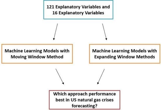
From the aforementioned literature, we can see that the methodologies proposed here offer clear innovations and advantages. Thus, we compared the predictive ability of the following models: XGboost, a SVM, a LogR, a RF, and a NN. In addition, we used a moving window and an expanding window approach. Furthermore, we investigated the effects of explanatory variables on the models’ predictive ability by splitting the variables into two categories—natural gas-related predictors (16 predictors), and all predictors (121 predictors)—to compare their prediction accuracy separately. To the best of our knowledge, our study is the first to analyze US natural gas market crises by combining machine learning techniques with dynamic forecasting methods (the moving window and expanding window method).

3. Data

3.1. Data Collection

We employed daily data to model US natural gas market crises, focusing on the US crude oil, stock, commodity, and agriculture markets, where the transmission of extreme events is stronger. In order to obtain an adequate daily data sample for machine learning, we collected data from many different sources and databases (see

Table 1. Variables in the model.

Variables	Raw Data	Data Source
Natural Gas	Henry Hub Natural Gas Futures (USD/Million Btu)	Bloomberg
Crude oil	Crude Oil WTI Futures (USD/Barrel)	Bloomberg
Stock	S&P 500 Index	Bloomberg
Bond	United States 10-Year Bond Yield	Bloomberg
Gold	Gold Futures Price	Bloomberg
Vix	CBOE Volatility Index	Bloomberg
Canola	Canola Futures Price	Bloomberg
Cocoa	US Cocoa Futures Price	Bloomberg
Sugar	No.11 Sugar Futures Price	Bloomberg
Rice	Rough Rice Futures Price	Bloomberg
Corn	Corn Futures Price	DataStream
Wheat	US Wheat Futures Price	DataStream

).

The raw data included the most sensitive market variables from the energy, stock, commodity, and agriculture markets. To remove the effect of the exchange rate on our results, we consolidated the currency units of the variables into a dollar currency unit. Then, because natural gas has the shortest period of daily data (8 June 1990–18 December 2019), we focused on this period for all variables. Finally, we obtained a raw daily price data set with 7152 records. This data set enabled us to model contagion dynamics and financial market interdependence across natural gas-related variables and over time. In order to facilitate the reading of this paper, we named the professional items as exhibited in

Table 2. Nomenclature for professional items.

Nomenclature
$p_t$	Natural Gas Daily Price
$r_t$	Natural Gas Daily Return
${\mu }_t$	1000-Day Moving and Expanding Window Average return at time $t$
${\sigma }_t$	1000-Day Moving and Expanding Window Standard deviation at time $t$
$N{C}_t$	US Natural gas crises at time $t$
XGboost	Extreme Gradient Boosting
SVM	Support Vector Machines
LogR	Logistic Regression
RF	Random Forests
NN	Neural Networks
G-mean	The geometric mean
LP	The positive likelihood ratio
LN	The negative likelihood ratio
DP	The discriminant power
BA	Balanced accuracy
WBA	The weighted balance accuracy
DM-test	Diebold-Mariano Test

.

3.2. Data Processing

In Section 3.1, we described the raw data and the prices of the variables. Our goal was to predict next-day crisis events in the US natural gas market using machine learning. Therefore, we needed to define a “crisis event” for natural gas. We also wanted to apply the moving window and expanding window methods in our model. We illustrate these two methods below (see

Table 3. Daily data set for the moving window and expanding window.

Variable Names	Numerical Formula
Natural Gas Daily Price	$p_t$
Natural Gas Daily Return	$r_t=\ln \left(p_t\right)-\ln \left(p_{t-1}\right)$
1000-Day Moving Window Average	${\mu }_{t+1000}=\frac{{\sum }_t^{t+999}{r}_t}{1000}$(t = 1, 2, …, 6151)
1000-Day Expanding Window Average	${\mu }_{i+1001}=\frac{{\sum }_1^{i+1000}{r}_t}{i+1000} (i=0,1,\dots 6150,t=1,2....6151$)
1000-Day Moving Window Standard Deviation	${\sigma }_{t+1000}=\sqrt{var(\sum _t^{t+999}{r}_t})$ (t = 1, 2, …, 6151)
1000-Day Expanding Window Standard Deviation	${\sigma }_{i+1001}=\sqrt{var(\sum _1^{i+1000}{r}_t}) \left(i=0,1,\dots 6150, t=1,2....6151\right)$

) [26].

We set a 1000-day window, covering five years of daily data. First, we employed the logarithmic difference method to compute the daily return of natural gas. Then, in the daily data set, we calculated the initial empirical distribution of the return on 22 September 1994, based on the daily returns of the first 1000 observations (covering the period 11 June 1990–21 September 1994, which is a 1000-day window). Next, for the moving window method, for each subsequent record, we fixed the number of days (1000 days in the daily data set), and moved the window forward by one day. Then, we recalculated the empirical distribution of the returns based on the new period. Thus, for the last observation in the daily data (18 December 2019), the empirical distribution of the returns was based on the period 23 November 2015 to 17 December 2019 (i.e., 1000 days). In contrast, for the expanding window method, for each subsequent record, we increased the size of the window by one day. Then, we again recalculated the empirical distribution of the returns, including the new observation. Hence, for the last observation in the daily data (18 December 2019), the empirical distribution of the returns was based on the period 11 June 1990, to 17 December 2019 (i.e., 7150 days).

Thus, we obtained the preliminary processed data from which to calculate the “crisis events.” Bussiere and Fratzscher [17] developed an EWS model based on a multinomial logit model to forecast financial crises, using $EM{P}_{i,t}$ to define a currency crisis for each country i and period t. Patel and Sarkar [27], Coudert and Gex [28], and Li et al. [29] used $CMA{X}_t$, defined as the ratio of an index level at month t to the maximum index level for the period up to month t. Here, we employed the return of natural gas, defined as follows:

$$r_t=ln\left(p_t\right)-ln\left(p_{t-1}\right),$$

(1)

where $p_t$ is the price of natural gas on day t. Next, as in Bussiere and Fratzscher [17], we defined $N{C}_t$ as a crisis event when the natural gas return $r_t$ is less than two standard deviations below its mean value:

$$N{C}_t=\{\begin{array}{c}1, if N{C}_t\le {\mu }_t-2{\sigma }_t\\ 0, otherwise\end{array},$$

(2)

where ${\mu }_t$ and ${\sigma }_t$ were calculated based on Table 3. The former is the mean value calculated by the moving window or expanding window on day t. Similarly, the latter denotes the standard deviation calculated by the corresponding methods. We plotted the crises processing procedure, as shown in Figure 2. After processing these data, we obtained two predicted/dependent variables in the daily data set. These constitute binary indicators that take the value of 1 when a crisis occurs in the US natural gas market on the following day, and 0 otherwise. Based on these formulae,

Table 4. Crisis events in the US natural gas market.

Year	Number of Crises
	Moving Window	Expanding Window
1994	2	2
1995	6	6
1996	16	18
1997	6	8
1998	3	4
1999	2	3
2000	6	7
2001	13	14
2002	3	3
2003	8	8
2004	3	5
2005	1	1
2006	7	8
2007	2	2
2008	7	5
2009	9	9
2010	0	0
2011	1	0
2012	3	2
2013	1	0
2014	10	4
2015	6	2
2016	7	0
2017	4	2
2018	10	7
2019	4	3
Total	140	123

and Figure 3 summarize the crisis events between 22 September 1994 and 18 December 2019.

We have outlined the exploratory binary variables in the daily data set using the moving window and expanding window methods. Next, we constructed the independent variables for our machine learning model. In particular, to capture the subtle dynamics and correlations, we performed the following transformation:

• We calculated the average number of crises during the previous five working days, based on the total number of crisis events.
• We used the logarithmic difference method to derive the continuously compounded daily return for the prices of natural gas, crude oil, bond yield, gold, canola, cocoa, sugar, rice, corn, and wheat.
• We calculated the lagged variables for each crisis indicator, for one to five days. Specifically, we considered these lags (lag1 to lag5) for the crisis itself, the returns on all variables except the VIX index, and the returns on all variables including the VIX index.

After the above processing, we obtained two summary tables of daily data for the period 28 February 1994 to 18 December 2019, yielding 6146 records and 121 predictors. The first table determines crises using the moving window method, and the second uses the expanding window method.

4. Model Development

As already discussed, we combined the moving window method, expanding window method, and machine learning to predict crisis events. In addition, we used a moving window and expanding window in the data processing step. Therefore, we employed corresponding methods to develop our model using machine learning. By doing so, we derived dynamic results and improved the accuracy of the model prediction [25]. To maintain the initial number of windows, we employed 1000 days as the initial number of days for the moving window (fixed) and the expanding window (increasing by one day). In order to combine machine learning with the two window methods, we inserted loop statements into the machine learning model to perform 5146 iterations. For both methods, we set all data in the window as the training data set, and set the day following the final day in the training data set as the test data set. For example, in the final loop calculation, the training data set for the moving window method covers the period 19 November 2015 to 17 December 2019 (1000 days), and the test data is that of 18 December 2019; for the expanding window method, the training data set covers the period 29 September 1994 to 17 December 2019 (6145 days), and the test data is that of 18 December 2019. Therefore, we derived a confusion matrix for crisis prediction once the loops were complete.

Next, we chose our methods following Chatzis et al. [23], deciding on the following: XGboost [30], SVM [31], LogR [32], RF [33,34,35], and NN [36]. We split the explanatory variables into two types to compare the predictions: A natural gas-related variable (the average number of crises during the previous five working days, lags 1 to 5 of crises, and lags 1 to 5 of the prices and returns of natural gas, yielding 16 predictors), and all variables (121 predictors, including natural gas-related variables). In the following section, we describe the development process and the parameter tuning for each model.

4.1. Extreme Gradient Boosting

XGboost is not only an improvement algorithm on the boosting algorithm based on gradient-boosted decision trees, and the internal decision tree uses a regression tree, but also an efficient and prolongable development of the gradient boosting framework [37]. It supports multiple kinds of objective functions, like regression, classification, ranking, and so on. Furthermore, in terms of model accuracy, efficiency, and scalability, XGboost outperforms RFs and NNs [23]. In our study, we employed the XGboost R package developed by Chen and He [30].

In order to increase the accuracy of the model prediction, we employed a (five-fold) cross-validation method to debug a series of vital hyperparameters. In order to build the classification tree, we determined the maximum depth of the tree, minimum number of observations in a terminal node, and size of the subsampling for both window methods. We also tuned the hyperparameter $\gamma$, which controls the minimum reduction in the loss function required to grow a new node in a tree, and reduces overfitting the model. In addition, we tuned $\alpha$ (the L1 regulation term on the weights) and $\lambda$ (the L2 regulation term on weights). Because of the binary nature of our dependent variable, we applied the LogR objective function for the binary classification to train the model. We also calculated the area under the curve (AUC) of our model, which is equal to the probability that the classifier ranks randomly selected positive instances higher than randomly selected negative instances. In our model training, when we employed the moving window method, the AUC values were above 0.8, regardless of whether we used 16 natural gas-related explanatory variables or 121 explanatory variables, indicating a very good performance. However, we derived an AUC of only 0.67 when applying the expanding window method, indicating a poor performance for the combination of this and the XGboost method.

Because we used the moving window and expanding window methods in our study, we cannot show every XGboost variable importance plot, because there were more than 5000 plots after the loop calculation. Therefore, we present the plots for the last step of the loop in the Appendix A. Here, Figure A1 and Figure A2 show that lag5 of the natural gas price is the most important variable in the moving window method. However, lag2 of the natural gas return is the most important in the expanding window method.

4.2. Support Vector Machines

Erdogan [38] applied an SVM [31] to analyze the financial ratio in bankruptcy, finding that the SVM with a Gaussian kernel is capable of predicting bankruptcy crises. This is because the SVM has a regularization parameter, which controls overfitting. Furthermore, using an appropriate kernel function, we can solve many complex problems. An SVM scales relatively well to high-dimensional data. Therefore, it is widely used in financial crisis prediction, handwriting recognition, and so on.

In our study, we used sigmoid, polynomial, radial basis function, and linear kernels to evaluate a soft-margin SVM, finding that the sigmoid function performs optimally. In order to select the optimal hyperparameter (e.g., $\gamma$, the free parameter of the Gaussian radial basis function, and c, the cost hyperparameter of the SVM, which involves a trading error penalty for stability), we applied cross-validation. We selected the optimal values of these hyperparameters using the grid-search methodology. We implemented the SVM model using the e1071 package in R, employing the tuning function in the e1071 package to tune the grid-search hyperparameter.

Unlike the XGboost methodology, we could tune the parameters $\gamma$ and c of the daily data set before executing the loop calculation. The plots of the parameter tuning for the SVM model are provided in the Appendix A. Figure A3 and Figure A4 show the hyperparameters $\gamma$ (x-axis) and c (y-axis) using the grid-search method in the SVM model. The parameter c is the cost of a misclassification. As shown, a large c yields a low bias and a high variance, because it penalizes the cost of a misclassification. In contrast, a small c yields a high bias and a low variance. The goal is to find a balance between “not too strict” and “not too loose”. For $\gamma$, the parameter of the Gaussian kernel, low values mean “far” and high values mean “close”. When $\gamma$ is too small, the model will be constrained and will not be able to determine the “shape” of the data. In contrast, an excessively large $\gamma$ will lead to the radius of the area of influence of the support vectors only including the support vector itself. In general, for an SVM, a high value of gamma leads to greater accuracy but biased results, and vice versa. Similarly, a large value of the cost parameter (c) indicates poor accuracy but low bias, and vice versa.

4.3. Logistic Regression

In statistics, the LogR algorithm is widely applied for modeling the probability of a certain class or event existing, such as crisis/no crisis, healthy/sick or win/lose, and so on. The LogR is a statistical model, which applies a logistic function to model a binary dependent variable in its basic form. Ohlson [32] employed a LogR to predict corporate bankruptcy using publicly available financial data. Yap et al. [39] employed a LogR to predict corporate failures in Malaysia over a 10-year period, finding the method to be very effective and reliable. In our study, we employed the glm function in R, following Hothorn and Everitt [40]. In addition, because the output of a LogR is a probability, we selected optimistic thresholds for the two window methods separately when predicting crises. We also employed a stepwise selection method to identify the statistically significant variables. However, this did not result in a good performance. Therefore, we did not consider the stepwise method further.

As before, we summarize some of the outcomes of our analysis in the Appendix A. Here,

Table A1. Estimated LogR model result: Partial variables.

Partial Variables
Moving Window Method					Expanding Window Method
	Estimate	Std. Error	z-Value	Pr(>|z|)		Estimate	Std. Error	z-Value	Pr(>|z|)
(Intercept)	−7.91	1.19	−6.65	2.91 × 10−11 ***	(Intercept)	−1.88 × 103	1.12 × 106	−0.002	0.999
crisis_ave5days	2.77	6.50	0.43	0.6698	crisis_ave5days	−8.71 × 102	7.42 × 105	−0.001	0.999
crisis_lag1	2.61	1.56	1.67	0.0942	crisis_lag1	2.19 × 102	1.23 × 105	0.002	0.999
hen_return_lag1	39.25	18.85	2.08	0.0373 *	hen_return_lag1	2.90 × 103	1.31 × 106	0.002	0.998

Notes: *** < 0.001 p-value; * < 0.05 p-value.

and

Table A2. Estimated LogR model result: All variables.

All Variables
Moving Window Method					Expanding Window Method
	Estimate	Std. Error	z-Value	Pr(>|z|)		Estimate	Std. Error	z-Value	Pr(>|z|)
(Intercept)	−4.56	0.21	−21.87	2 × 10−16 ***	(Intercept)	−5.48	1.73	−3.17	0.00153 **
crisis_ave5days	8.75	2.34	3.73	0.000190 ***	crisis_ave5days	7.30	2.58	2.83	0.00465 **
hen_return_lag5	7.31	2.21	3.31	0.000944 ***	hen_return_lag5	6.60	2.39	2.76	0.00582 **
hen_return_lag2	9.19	4.07	2.26	0.023885 *	gold_return_lag5	2.61	9.88	2.64	0.00835 **

Notes: *** < 0.001 p-value; ** < 0.01 p-value; * < 0.05 p-value.

exhibit some of the outcomes of our analysis and we also present the plot of the final step of the loop calculation, showing only the intentionality of some of the variables. As shown, whether in the partial variables case or the all variables case, the lagged value and the average of five days of crisis are the most intentional.

4.4. Random Forests

An RF [33,34,35] is an advanced learning algorithm employed for both classification and regression created by Ho [41]. A forest in the RF model is made up of trees, where a greater number of trees denotes a more robust forest. The RF algorithm creates decision trees from data samples, obtains a prediction from each, and selects the best solution by means of voting. Compared with a single decision tree, this is an ensemble method. Because it can reduce overfitting by averaging the results. RFs are known as bagging or bootstrap aggregation methods. By identifying the best segmentation feature from the random subset of available features, further randomness can be introduced.

In RF, a large number of predictors can provide strong generalization; our model contains 121 predictors. In order to improve the accuracy of model prediction, we must obtain an optimal value of m, the number of variables available for splitting at each tree node. If m is relatively low, then both the inter-tree correlation and the strength of each tree will decrease. To find the optimal value, we employed the grid-search method. In addition to m, we tuned the number of trees using the grid-search method. To reduce the computing time, we applied the ranger package in R to construct the prediction model, employing the tuneRF function in the randomForest package.

We provide the RF variable importance plots in the last loop calculation in Appendix A. In Figure A5 and Figure A6, we present the importance of each indicator for the classification outcome. The obtained ranking is based on the mean decrease in the Gini. This is the average value of the total reduction of variables in node impurities, weighted by the proportion of samples that reach the node in each decision tree in RF. Here, a higher mean decrease in the Gini indicates higher variable importance. We found that in the partial variables case, the lags of the natural gas price and the natural gas return are relatively important; however, in the case of all variables, this was not the case.

4.5. Neural Networks

In the field of machine learning and cognitive science, an NN [34] is a mathematical or computational model, which imitates the structure and function of a biological neural network (animal central nervous system, especially the brain), employed to estimate or approximate functions. Like other machine learning methods, NN have been used to solve a variety of problems, such as credit rating classification problems, speech recognition, and so on. The most usually considered multilayer feedforward network is composed of three types of layers. First, in the input layer, many neurons accept a large number of nonlinear input messages. The input message is called the input vector. Second, the hidden layer, which is the various layers composed of many neurons and links between the input layer and output layer. The hidden layer can have one or more layers. The number of neurons in the hidden layer is indefinite, but the greater the number, the more nonlinear the NN becomes, so that the robustness of the neural network is more significant. Third, in the output layer, messages are transmitted, analyzed, and weighed in the neuron link to form the output. The output message is called the output vector.

In order to increase the accuracy of the model prediction, we employed the grid-search method to find the best parameter size and decay. The parameter size is the number of units in the hidden layer and parameter decay is the regularization parameter to avoid over-fitting. We used nnet package in R to develop the model prediction.

5. Model Evaluation

In this section, we evaluate the robustness of our methods by performing a comprehensive experimental evaluation procedure. Specifically, we use several criteria to evaluate the aforementioned models in terms of crisis event prediction.

5.1. Verification Methods

Accuracy is measured by the discriminating power of the rating power of the rating system. It is the most commonly used indicator for classification, and it estimates the overall effectiveness of an approach by estimating the probability of the true value of the class label. In the following section, we introduce a series of indicators that are widely employed to quantitatively estimate the discriminatory power of each model.

In machine learning, we can derive a square 2 × 2 matrix, as shown in

Table 5. Confusion matrix for two classes classification.

	Predicted 0	Predicted 1
Actual 0	TN (number of True Negatives)	FP (number of False Positives)
Actual 1	FN (number of False Negatives)	TP (number of True Positives)

Notes: 0 refers to “No crisis”; 1 refers to “Crisis”; Predicted 0 refers to a predicted value of 0, Predicted 1 refers to a predicted value of 1; Actual 0 refers to a true value of 0; Actual 1 refers to a true value of 1; TN = True Negative: the number of negative cases (i.e., no crisis) correctly identified as negative cases; FP = False Positive: the number of negative cases (i.e., no crisis) incorrectly identified as positive cases; FN = False Negative: the number of positive cases (i.e., crisis) misclassified as negative cases; TP = True Positive: the number of positive cases (i.e., crisis) correctly identified as positive.

, which we used as the basis of our research.

Bekkar et al. [42] state that imbalanced data learning is one of the challenging problems in data mining, and consider that skewed classes in the level distribution can lead to misleading assessment methods and, thus, bias in the classification. To resolve this problem, they present a series of alternatives for imbalanced data learning assessment, which we introduce below.

Bekkar et al. [42] defined sensitivity and specificity as follows:

$$Sensitivity\left(orRecall\right)=\frac{TP}{TP+FN};Specificity=\frac{TN}{TN+FP}.$$

(3)

Sensitivity and specificity assess the effectiveness of an algorithm on a single class for positive and negative outcomes, respectively. The evaluation measures are as follows:

• G-mean: The geometric mean is the product of the sensitivity and specificity. This metric can indicate the valance between the classification performance of the majority and minority classes. In addition, the G-mean measures the degree to which we avoid overfitting on the negative class, and the degree to which the positive class is marginalized. The formula is as follows:

  $$G-\mathit{mean}=\sqrt{Sensitivity\times Specificity}.$$

  (4)

Here, a low G-mean value means the prediction performance of the positive cases is poor, even if the negative cases are correctly classified by the algorithm.

• LP: The positive likelihood ratio is that between the probability of predicting an example as positive when it is really positive, and the probability of a positive prediction when it is not positive. The formula is as follows:

  $$LP=\frac{TP/\left(TP+FN\right)}{FP/\left(FP+TN\right)}=\frac{Sensitivity}{1-Specificity}.$$

  (5)
• LN: The negative likelihood ratio is that between the probability of predicting an example as negative when it is really positive, and the probability of predicting a case as negative when it is actually negative. The formula is as follows:

  $$LN=\frac{FN/\left(TP+FN\right)}{TN/\left(FP+TN\right)}=\frac{1-Sensitivity}{Specificity}.$$

  (6)
• DP: The discriminant power, a measure that summarizes sensitivity and specificity. The formula is as follows:

  $$DP=\frac{\sqrt{3}}{\pi }\left(log\frac{Sensitivity}{1-Sensitivity}-log\frac{Specificity}{1-Specificity}\right).$$

  (7)

DP values can evaluate the degree to which the algorithm differentiates between positive and negative cases. DP values lower than one indicate that the algorithm differentiates poorly between the two, and values higher than three indicate that it performs well.

• BA: Balanced accuracy, calculated as the average of the sensitivity and specificity. The algorithm is as follows:

  $$BA=\frac{1}{2}\left(Sensitivity+Specificity\right).$$

  (8)

If the classifier performs equally well in both classes, this term reduces to the conventional accuracy measure. However, if the classification performs well in the majority class (in our study, “no crisis”), the balance accuracy will drop sharply. Therefore, the BA considers the majority class and minority class (in our study, “crisis”) equally.

• WBA: The weighted balance accuracy. Under the weighting scheme 75%: 25%, the WBA emphasizes sensitivity over specificity, and is defined by Chatzis et al. [23] as follows:

  $$WBA=0.75\ast Sensitivity+0.25\ast Specificity.$$

  (9)
• Youden’ s $\gamma$: An index that evaluates the ability of an algorithm to avoid failure. This index incorporates the connection between sensitivity and specificity, as well as a linear correspondence with balanced accuracy:

  $$\gamma =Sensitivity-\left(1-Specificity\right)=2\ast BA-1.$$

  (10)
• F-measure: The F-measure employs the same contingency matrix as that of relative usefulness. Powers [43] shows that an optimal prediction implies an F-measure of one. The formula is as follows:

  $$F-\mathit{measure}=\frac{TP}{TP+\frac{\left(FP+FN\right)}{2}}.$$

  (11)
• DM-test: The Diebold–Mariano test is a quantitative approach to evaluate the forecast accuracy of US natural gas crises predicting models in our paper [44]. In our paper, the DM-test can help us to discriminate the significant differences of the predicting accuracy between the XGboost, SVM, LogR, RF, and NN models based on the scheme of quantitative analysis and about the loss function. We employed the squared-error loss function to do the DM-test.

To simplify the explanation of its values, the F-measure was defined such that a higher value of $\mathsf{\gamma }$ indicates a better ability to avoid classifying incorrectly.

After a series of illustrations of the algorithm above, we derived a variety of methods to evaluate the model prediction ability. Here, we used all of the methods to derive a comprehensive and accurate view of the models’ performance. Lastly, we calculated an optimal US natural gas market collapse probability critical point for each fitted model, thus obtaining the optimal sensitivity and specificity measures. We focused on false negatives rather than false positives, because the goal of our work was to construct a supervised warning mechanism, which can predict as many correct signals as possible while reducing the incidence of false negatives.

5.2. Models Prediction Results

We identified 121 predictors and 6146 records for the period 29 September 1994 to 18 December 2019. In addition to using the two window methods, we determined the performance of the models when predicting US natural gas crises using natural gas-related predictors only (16 predictors) and all predictors (121 predictors) separately. In the following, we refer to the combination of the moving window method and the natural gas-related predictors as the “partial variables with the moving window” method. Similarly, we have the “partial variables with expanding window” method. When we combined the moving window method with all variables, we have the “all variables with a moving window” method and, similarly, we have the “all variables with an expanding window” method.

As shown in

Table 6. Verification methods: Dependent variable concerns a US natural gas crisis (partial variables).

Partial Variables
Moving Window Method						Expanding Window Method
	XGboost	SVM	LogR	RF	NN		XGboost	SVM	LogR	RF	NN
G-mean	0.617	0.353	0.460	0.328	0.377	G-mean	0.589	0.419	0.493	0.300	0.489
LP	2.523	4.556	3.032	5.384	4.427	LP	2.912	4.135	3.215	3.877	4.618
LN	0.653	0.897	0.834	0.908	0.882	LN	0.694	0.854	0.802	0.930	0.790
DP	0.745	0.896	0.712	0.981	0.889	DP	0.791	0.870	0.766	0.787	0.973
BA	0.641	0.550	0.577	0.545	0.557	BA	0.632	0.570	0.591	0.534	0.599
WBA	0.555	0.339	0.403	0.327	0.352	WBA	0.517	0.377	0.428	0.313	0.426
Youden	0.282	0.100	0.154	0.090	0.114	Youden	0.264	0.139	0.182	0.068	0.198
F-measure	0.093	0.106	0.097	0.107	0.110	F-measure	0.085	0.098	0.087	0.074	0.114

Notes: “Partial variables” refers to 16 natural gas-related explanatory variables. G-mean (geometric mean), LP (positive likelihood ratio), LN (negative likelihood ratio), DP (discriminant power), BA (balanced accuracy), weighted balanced accuracy (WBA), Youden (Youden’s $\gamma$), F-measure.

and

Table 7. Verification methods: Dependent variable concerns a US natural gas crisis (all variables).

All Variables
Moving Window Method						Expanding Window Method
	XGboost	SVM	LogR	RF	NN		XGboost	SVM	LogR	RF	NN
G-mean	0.605	0.374	0.387	0.325	0.357	G-mean	0.541	0.460	0.448	0.278	0.330
LP	1.958	2.993	1.797	2.705	1.858	LP	2.742	1.948	2.682	2.035	2.092
LN	0.684	0.897	0.919	0.928	0.931	LN	0.759	0.866	0.851	0.957	0.937
DP	0.580	0.664	0.369	0.590	0.381	DP	0.708	0.447	0.633	0.416	0.443
BA	0.619	0.549	0.537	0.535	0.532	BA	0.606	0.559	0.568	0.520	0.530
WBA	0.553	0.348	0.351	0.322	0.335	WBA	0.470	0.400	0.393	0.300	0.322
Youden	0.238	0.098	0.073	0.069	0.064	Youden	0.212	0.117	0.137	0.041	0.060
F-measure	0.075	0.086	0.061	0.074	0.060	F-measure	0.079	0.057	0.073	0.048	0.053

Notes: “All variables” refers to all 121 explanatory variables. G-mean (geometric mean), LP (positive likelihood ratio), LN (negative likelihood ratio), DP (discriminant power), BA (balanced accuracy), weighted balanced accuracy (WBA), Youden (Youden’s $\gamma$), F-measure.

, when we applied the partial explanatory variables (16 variables) to develop the machine learning models, XGboost provided the best empirical performance for both window methods, followed by the LogR in the moving window method and NN in the expanding window method since the Youden’s $\mathsf{\gamma }$ of XGboost was the highest in both two window methods, which means that XGboost has a better ability to avoid misclassification. Furthermore, the BA and WBA of XGboost was also the highest, which means that XGboost performs well in both crises’ prediction and no-crisis forecasting. When we employed all explanatory variables (121 variables), XGboost clearly still performed best in both dynamic methods, followed by the SVM in the moving window and LogR in the expanding window from Youden’s $\mathsf{\gamma }$ values. Similarly, the BA and WBA of XGboost was also the highest in the all variables situation.

In addition, because Table 6 and Table 7 show that the forecasting performances of XGboost are great and far exceed the other four models, when implementing the DM-test, we only evaluated the forecast accuracy between XGboost and the other four models. From

Table 8. The results of the Diebold–Mariano test (partial variables).

Partial Variables
Moving Window Method
	XGboost&SVM	XGboost&LogR	XGboost&RF	XGboost&NN
DM-test	30.138	22.655	24.383	25.848
p-value	p < 2.2 × 10−16	p < 2.2 × 10−16	p <2.2 × 10−16	p < 2.2 × 10−16
Expanding Window Method
	XGboost&SVM	XGboost&LogR	XGboost&RF	XGboost&NN
DM-test	20.483	13.871	23.793	21.684
p-value	p < 2.2 × 10−16	p < 2.2 × 10−16	p <2.2 × 10−16	p < 2.2 × 10−16

Notes: DM-test means Diebold–Mariano test. We employ the squared-error loss function to do the DM-test.

and

Table 9. The results of the Diebold–Mariano test (all variables).

All Variables
Moving Window Method
	XGboost&SVM	XGboost&LogR	XGboost&RF	XGboost&NN
DM-test	31.334	20.68	29.858	23.673
p-value	p < 2.2 × 10−16	p < 2.2 × 10−16	p < 2.2 × 10−16	p < 2.2 × 10−16
Expanding Window Method
	XGboost&SVM	XGboost&LogR	XGboost&RF	XGboost&NN
DM-test	8.4212	15.986	23.138	20.041
p-value	p < 2.2 × 10−16	p < 2.2 × 10−16	p < 2.2 × 10−16	p < 2.2 × 10−16

Notes: DM-test means Diebold–Mariano test. We employ the squared-error loss function to do the DM-test.

, we can see from the results of DM-test that in both the partial variables and all variables situations and whether by the moving window method or expanding window method, according to the DM-test based on the squared-error loss, all the DM-test values >1.96, the zero hypothesis is rejected at the 5% level of significance; that is to say, the observed differences between XGboost and other four models are significant and XGboost in US natural gas crises prediction accuracy is best between the five models used in our paper.

Summarizing the results across the five model evaluations in the test sample, it is evident that XGboost outperforms the other machine learning models. So far, there are very few papers related to forecasting US natural gas crises through machine learning. Thus, our research has made a certain contribution to the prediction of US natural gas crises.

5.3. Confusion Matrix Results

Referring to Chatzis et al. [23], we computed the final classification performance confusion matrices for the evaluated machine learning models (see

Table 10. Confusion matrix results: Partial variables.

Partial Variables
Moving Window Method					Expanding Window Method
XGboost	Predict					Predict
TRUE	0	1	Signal		TRUE	0	1	Signal
0	4103	934	False alarm	19%	0	4360	699	False alarm	15%
1	58	51	Hit rate	47%	1	52	35	Hit rate	40%
SVM	Predict					Predict
TRUE	0	1	Signal		TRUE	0	1	Signal
0	4895	142	False alarm	5%	0	4834	225	False alarm	6%
1	95	14	Hit rate	13%	1	71	16	Hit rate	18%
LogR	Predict					Predict
TRUE	0	1	Signal		TRUE	0	1	Signal
0	4656	381	False alarm	9%	0	4643	416	False alarm	9%
1	84	25	Hit rate	23%	1	64	23	Hit rate	26%
RF	Predict					Predict
TRUE	0	1	Signal		TRUE	0	1	Signal
0	4934	103	False alarm	4%	0	4939	120	False alarm	4%
1	97	12	Hit rate	11%	1	79	8	Hit rate	9%
NN	Predict					Predict
TRUE	0	1	Signal		TRUE	0	1	Signal
0	4870	167	False alarm	5%	0	4782	277	False alarm	7%
1	93	16	Hit rate	15%	1	65	22	Hit rate	25%

and

Table 11. Confusion matrix results: All variables.

All Variables
Moving Window Method					Expanding Window Method
XGboost	Predict					Predict
TRUE	0	1	Signal		TRUE	0	1	Signal
0	3786	1251	False alarm	25%	0	4444	615	False alarm	13%
1	56	53	Hit rate	49%	1	58	29	Hit rate	33%
SVM	Predict					Predict
TRUE	0	1	Signal		TRUE	0	1	Signal
0	4790	247	False alarm	7%	0	4432	627	False alarm	13%
1	93	16	Hit rate	15%	1	66	21	Hit rate	24%
LogR	Predict					Predict
TRUE	0	1	Signal		TRUE	0	1	Signal
0	4574	463	False alarm	11%	0	4647	412	False alarm	9%
1	91	18	Hit rate	17%	1	68	19	Hit rate	22%
RF	Predict					Predict
TRUE	0	1	Signal		TRUE	0	1	Signal
0	4832	205	False alarm	6%	0	4859	200	False alarm	5%
1	97	12	Hit rate	11%	1	80	7	Hit rate	8%
NN	Predict					Predict
TRUE	0	1	Signal		TRUE	0	1	Signal
0	4664	373	False alarm	9%	0	4781	278	False alarm	7%
1	94	15	Hit rate	14%	1	77	10	Hit rate	11%

). Here, a false alarm means a false positive rate, and the hit rate denotes the proportion of correct crisis predictions in the total number of crises. For the best performing model, XGboost, we found that the false alarms do not exceed 25%, and the highest hit rate is 49%. Thus, our US natural gas crisis prediction accuracy can reach 49% using all variables with the moving window method.

6. Conclusions

We proposed a dynamic moving window and expanding window method that combines XGboost, an SVM, a LogR, an RF, and an NN as machine learning techniques to predict US natural gas crises. We proposed the following full procedure. First, we selected the most significant US natural gas financial market indicators, which we believe can be employed to predict US natural gas crises. Second, we combined the aforementioned dynamic methods with other methods (e.g., the returns and lags of the raw prices) to process the daily data set, and defined a crisis for the machine learning model. Third, we used the five machine learning models (XGboost, SVM, LogR, RF, and NN) with dynamic methods to forecast the crisis events. Finally, we evaluated the performance of each model using various validation measures. We demonstrated that combining dynamic methods with machine learning models can achieve a better performance in terms of predicting US natural gas crises. In addition, our empirical results indicated that XGboost with the moving window method achieves a good performance in predicting such crises.

Our main conclusions can be summarized as follows. From the various verification methods, DM-test results, and confusion matrix results, XGboost with a moving window approach achieved a good performance in predicting US natural gas crises, particularly in the partial variables case. In addition, LogR in the moving window method and NN in the expanding window method did not perform badly in the partial variables situation whereas SVM in the moving window and LogR in the expanding window did not perform badly in the all variables situation. Our conclusions can help us to forecast the crises of the US natural gas market more accurately. Because financial markets are contagious, policymakers must consider the potential effect of a third market. This is equally important for asset management investors, because diversified benefits may no longer exist during volatile times. Therefore, these findings can help investors and policymakers detect crises, and thus take preemptive actions to minimize potential losses.

The novel contributions of our study can be summarized as follows. First, to the best of our knowledge, this study is the first to combine dynamic methodologies with machine learning to predict US natural gas crises. A lot of the previous studies are about the currency exchange crises, bank credit crises, and so on. So far, there are very few papers related to forecasting US natural gas crises through machine learning. Second, we implemented XGboost, a popular and advanced machine learning model in the financial crisis prediction field. Additionally, we found that XGboost outperforms in forecasting US natural gas crises. Third, we employed various parameter tuning methods (e.g., the grid-search) to improve the prediction accuracy. Fourth, we used novel evaluation methods appropriate for imbalanced data sets to measure the model performance and we also employed the DM-test method and found that the forecasting performance of XGboost is significant. Finally, we employed in-depth explanatory variables that cover the spectrum of major financial markets.

Before combining the dynamic methodologies with machine learning techniques, we performed ordinary machine learning, in that 70% of the data was used as training data and 30% was used as test data. However, the prediction performance of this method was not so satisfactory. Although our research is the first to combine machine learning techniques with dynamic methodologies for US natural gas crisis prediction, the prediction accuracy of our model can be improved. This is left to future research. Lastly, because economic conditions change continuously and crises continue to occur, predicting crisis events will remain an open research issue.