6.1. Model of the Building
This subsection describes the proposed model to estimate the
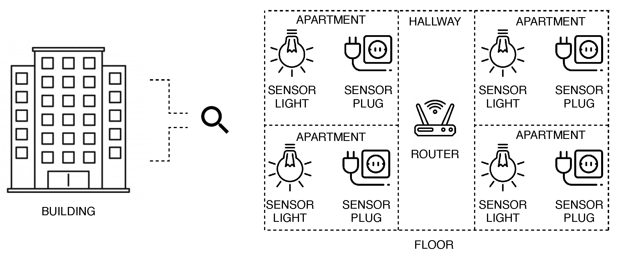
to a single floor. The components that composed a single floor were described in
Figure 5. Therefore, we have smart plug, smart light, and router. We recognize that the
and
(
and
of the floor subsystem) are exponentially distributed. Therefore, the
can be estimated by integrating reliability as a time function described in Equation (
15), while the system’s
can be obtained from the repair team’s reported data.
Reliability can be obtained by Equation (
16), where
is the immediate failure rate of the subsystem, considering that a single failure in any component brings the whole subsystem down. The
can be obtained by summing all immediate failure rates of all components, as shown by Equation (
17), where
,
, and
are the failure rate of the smart plugs, light meter sensors and router respectively.
where
X represents the number of smart plugs,
Y the number of light meter sensors, and
Z the number of routers.
It is deserving declaring that the mathematical representations presented in this subsection are generic. Therefore, it allows each designer to represent the appropriate environment for each situation.
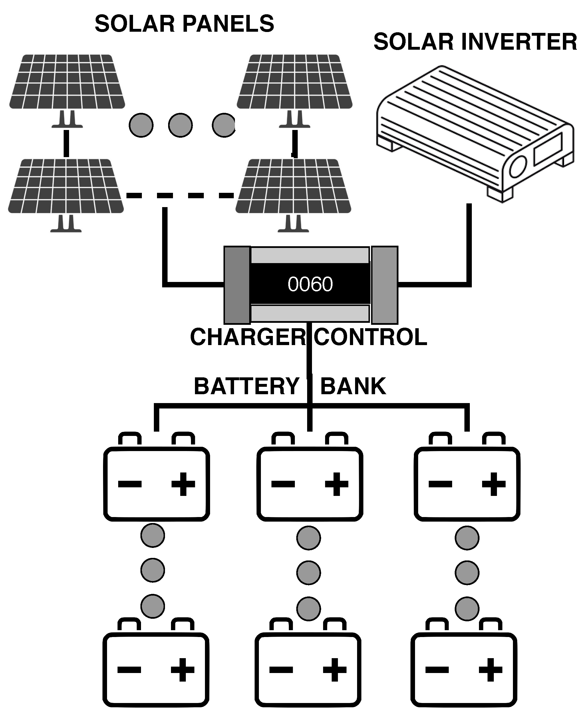
6.2. Model of the Hybrid Solar System
This subsection describes the proposed model to calculate the
to a hybrid solar power system.
Figure 3 describe the environment proposed, with the exception of the sensors present on the battery bank, on photovoltaic panels, and on the utility grid, as shown in
Figure 4. Therefore, we have photovoltaic panels, batteries, inverter, charge control, sensors on panels, battery bank, and utility grid. We consider that the
and
(
and
of the solar subsystem) are exponentially distributed. Therefore, the
can be estimated by the reliability integration as a time function, as expressed in Equation (
18), while the system’s
can be obtained from the repair team’s reported data.
Reliability can be obtained by Equation (
19), where
is the immediate failure rate of the subsystem, considering that a single failure in any component brings the whole subsystem down. The
can be obtained by summing all immediate failure rates of all components, as shown by Equation (
20), where
,
,
,
,
,
, and
are the failure rate of the solar panel, charge controller, battery, inverter, panel sensor, battery sensor, and utility grid sensor, respectively.
where
X represents the number of panels,
Y the number of batteries,
Z the number of inverters, and
W number of charger controls.
As in the previous subsection, the mathematical model presented here is generic. Therefore, the designer can manipulate the equations to represent a hybrid photovoltaic park as needed.
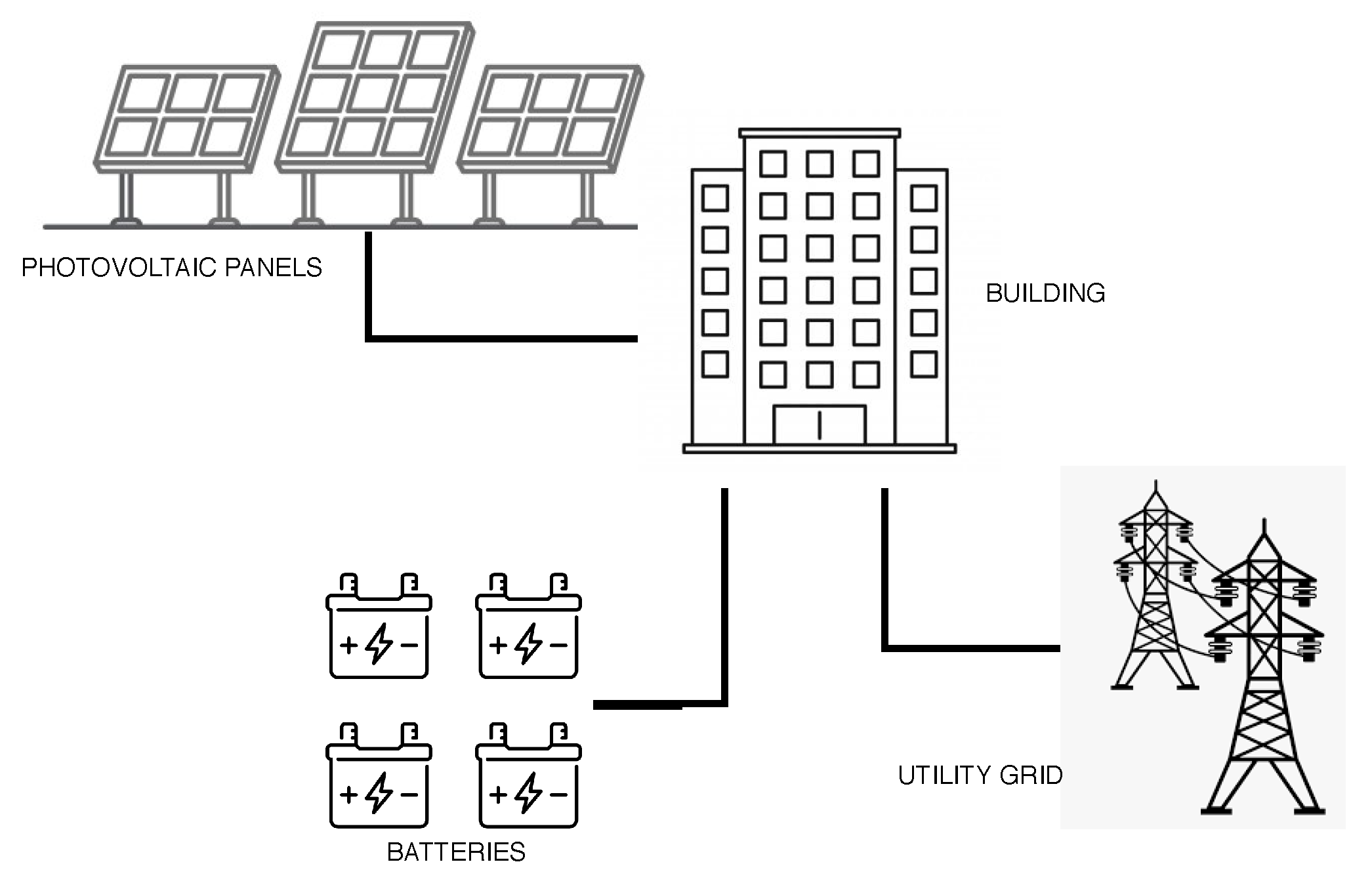
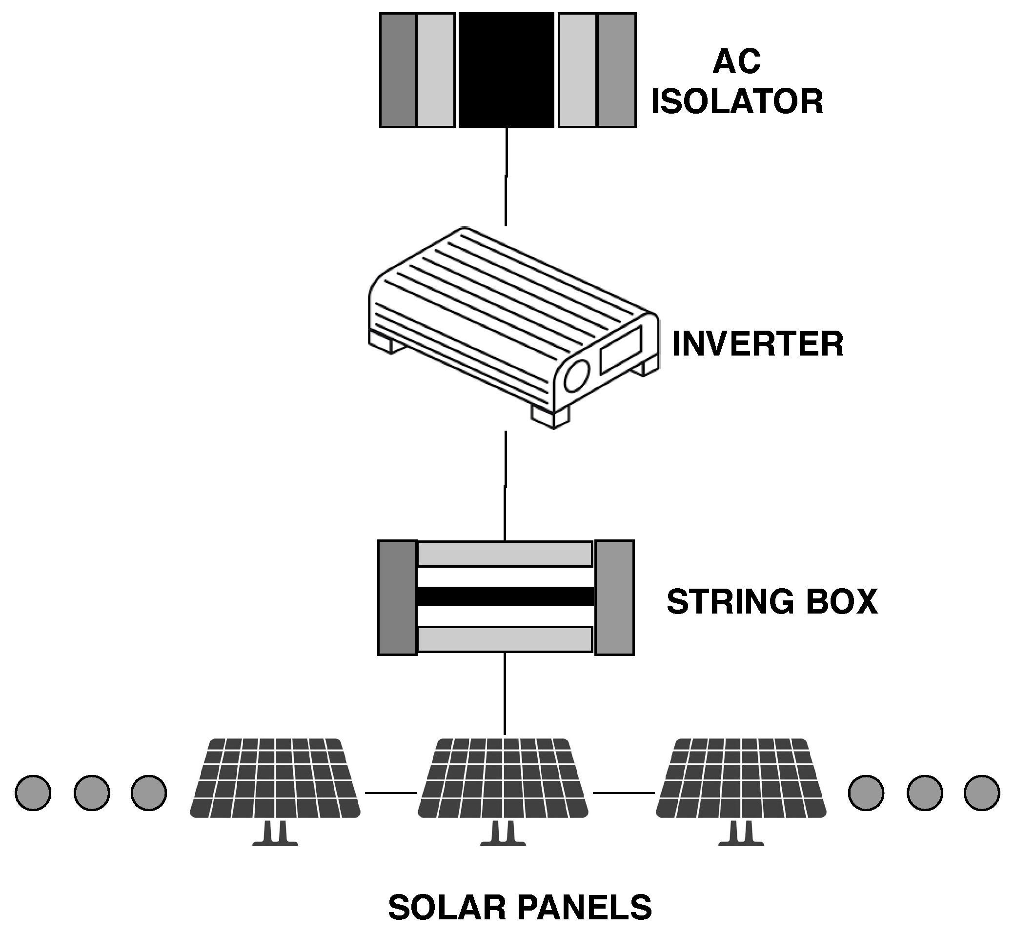
6.3. Model of Grid-Tie Solar System
This subsection describes the proposed model to calculate the
to a grid-tie solar power system. It is deserving of declaration that the generic models presented in this subsection can be adapted to any grid-tie photovoltaic system.
Figure 2 describe the environment proposed, with the exception of the sensors present on the on photovoltaic panels and on the utility grid, as shown in
Figure 4. Therefore, we have photovoltaic panels, AC isolator, inverter, string box, sensors on panels, and sensor on the utility grid. We recognize that the
and
(
and
of the solar subsystem) are exponentially distributed. Therefore, the
can be estimated by the reliability integration as a time function, as expressed in Equation (
21), while the system’s
can be obtained from the repair team’s reported data.
Reliability can be obtained by Equation (
22), where
is the immediate failure rate of the subsystem, considering that a single failure in any component brings the whole subsystem down. The
can be obtained by summing all immediate failure rates of all components, as shown by Equation (
23), where
,
,
,
,
, and
are the failure rate of the solar panel, AC isolator, string box, solar inverter, panel sensor, and utility grid sensor respectively.
where
X represents the number of panels,
Y number of AC isolators,
Z number of string box, and
W number of inverters.
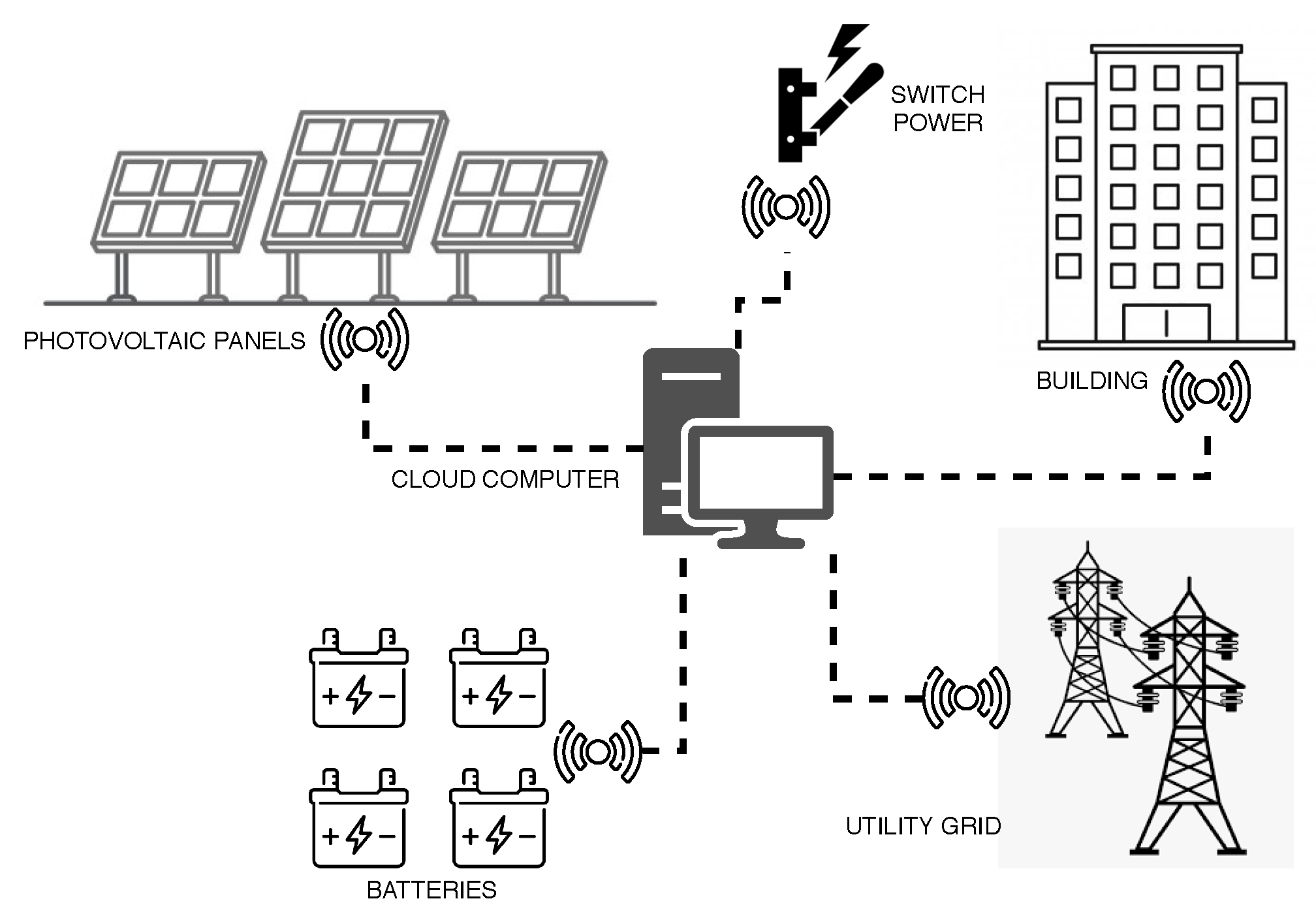
6.4. SPN Availability Model of the Entire System
This section details the planned availability model for the whole system regarding a redundant local management infrastructure.
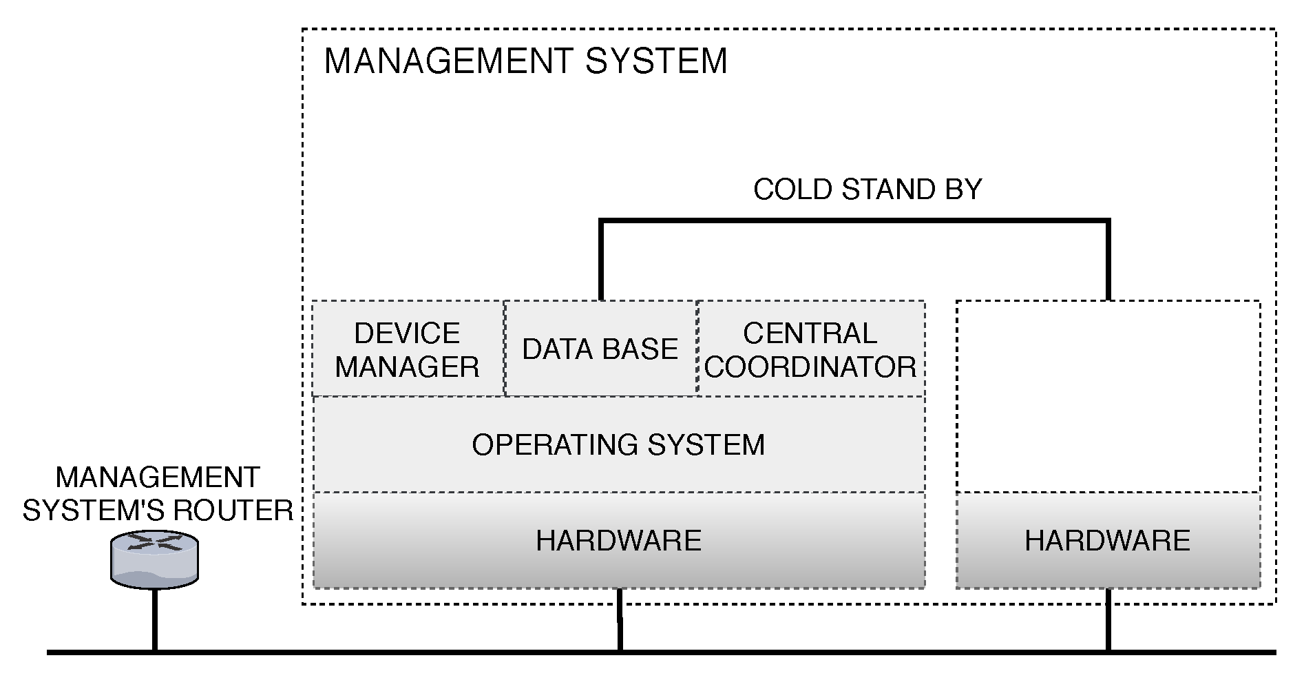
Figure 7 shows the management system infrastructure.
This local infrastructure contains the minimum requirements with redundancy for the operation of the proposed system. However, to ensure greater availability, we adopt a cold standby redundancy system, so the secondary machine acts as a backup of the main machine. Therefore, the necessary O.S. and software environment setup will only be made after the primary break down of the first machine. Accordingly, to achieve availability metrics, we recognize six elements, router, hardware, operating system, device manager, database, and central coordinator. The device manager is an application capable of controlling every component besides conceiving the information analytically. A central coordinator is a software that analyzes the energy consumption and the energy generated by the solar energy system in order to activate or deactivate the solar energy system.
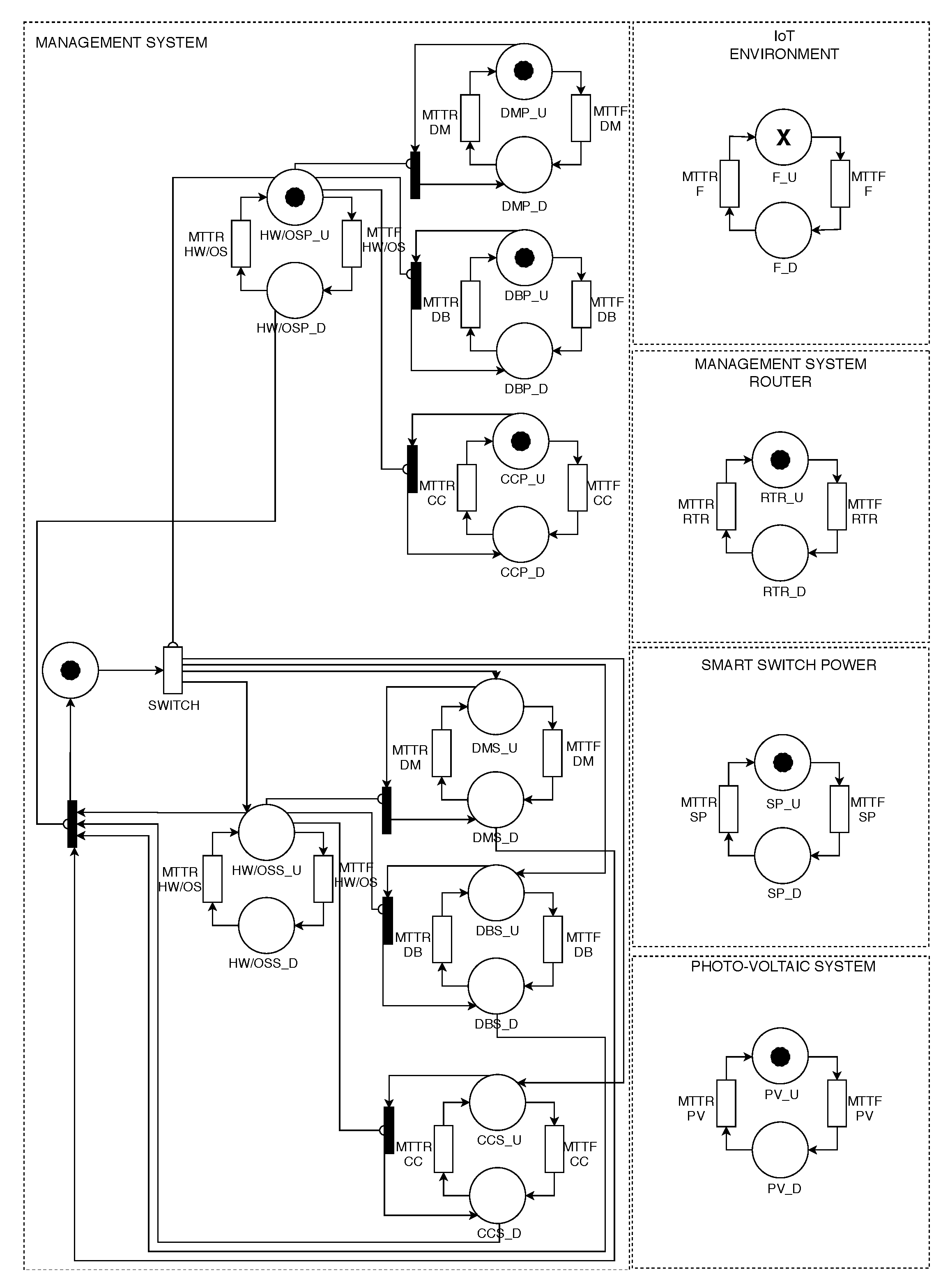
A Stochastic Petri Net (SPN), depicted in
Figure 8, was developed to describe the cold-standby redundancy system, discriminated through regarding a non-negligible interval during switching among the computers in the appearance of a crash in one of them. The principal machine will ever become preference over another machine. The model also describes the solar power system and the internet of things environment. Therefore, it is possible to use the “same” model to evaluate both. However, it is necessary to use the corresponding
and
values for each model of the solar power system. The smart switch power and the router responsible for sending the environment data to the management system also presented in the model. The SPN model was used because it allows transitions with delay values exponentially distributed, which is necessary to represent the proposed system accurately. Besides, it enables the representation of system behavior and evaluation of required metrics simply and concisely.
The redundancy system comprises Hardware and Operating System (HW/OS), Device Manager (DM), Central controller (CC) and Database (DB). We assume, for the initial system state, that the primary server is operating, which is described through a token in the place: HW/OSP_U (hardware and operating system are up), DMP_U (device manager is up), CCP_U (central controller is up), and DBP_U (database is up). Every element has an MTTF, whose value is assigned to delay of its respective transition: MTTF_HW/OS (MTTF hardware and operating system), MTTF_DM (device manage’s MTTF), MTTF_CC (central controller’s MTTF), and MTTF_DB (database’s MTTF). These transitions follow a single-server semantic and their firing delays are exponentially distributed. The single-server semantic does not allow multiple firing events when the degree of activation is greater than one, i.e., the transition fires only once at a time. Therefore, when a component fails, the corresponding transition consumes a token from its “up” place to its “down” place. The failure of those components is denoted by the following places: DMP_D (DM is down), CCP_D (CC is down), DBP_D (DB is down), and HW/OSP_D (hardware and operating are down). When a component is down, it might be repaired by the maintenance team. Every element has an MTTR in some transitions in the model: HW/OS_MTTR (MTTR hardware and operating system), DM_MTTR (device manage’s MTTR), CC_MTTR (central controller’s MTTR), and DB_MTTR (database’s MTTR). These transitions also follow a single-server semantic and their firing delays are exponentially distributed. Therefore, when the component is down the transition may fire according to its MTTR, pulling out a token from the “down” place to the “up” place. However, when the primary server (hardware and operating system) fails, the SWITCH transition fires, making the auxiliary server move from the inactive state to enter the active state. This transition describes the moment to turn on the auxiliary server and transfer the workload to it, which takes less time than the time to repair the primary server. The second server is represented by the places: HW/OSS_U (hardware and operating system are up), DMS_U (device manager is up), CCS_U (central controller is up), and DBS_U (database is up). The failure of those components is denoted by the following places: DMS_D (DM is down), CCS_D (CC is down), DBS_D (DB is down), and HW/OSS_D (hardware and operating are down). The
can be estimated by integrating reliability as a time function, as expressed in Equation (
24), whereas the system’s MTTRs can be obtained from the data reported from the repair team.
Reliability can be obtained by Equation (
25), where
is the immediate failure rate of all subsystem components. The
can be obtained by summing all immediate failure rates of all components, as shown by Equation (
26), where
and
are the failure rate of the hardware, and operating system, respectively.
The
and
places described the building environment. The
place represents that every element is active. Whereas, the
Figure 5 describe only one floor of the building, this SPN model represents all floors we want, by the quantity of token in the
place represent by X. The MTTF and MTTR of the building environment on a floor are represented in transitions F_MTTF and F_MTTR, respectively. The firing delay of F_MTTF transition corresponds to an exponential distribution, and the transition follows an infinite-server semantic, which enables the transition to fire multiple times simultaneously if there are enough tokens and the timing of events allows that. Therefore, it represents properly the fact that the failures of each floor subsystem are independent of each other. The F_MTTR transition corresponds to an exponential distribution and follows a single-server semantic.
The solar power system is described by
and
places. The
place symbolizes that every element of the solar power system is active. The MTTF and MTTR of the solar power system are represented in transitions PV_MTTF and PV_MTTR, respectively. These transitions also follow a single-server semantic, and their firing delays are exponentially distributed. Whereas, the
Section 7.1.1 and
Section 7.1.2 presented how the values of the transitions were obtained. The smart switch power sensor, which exchanges the electrical energy to solar energy and vice and versa, is represented by
and
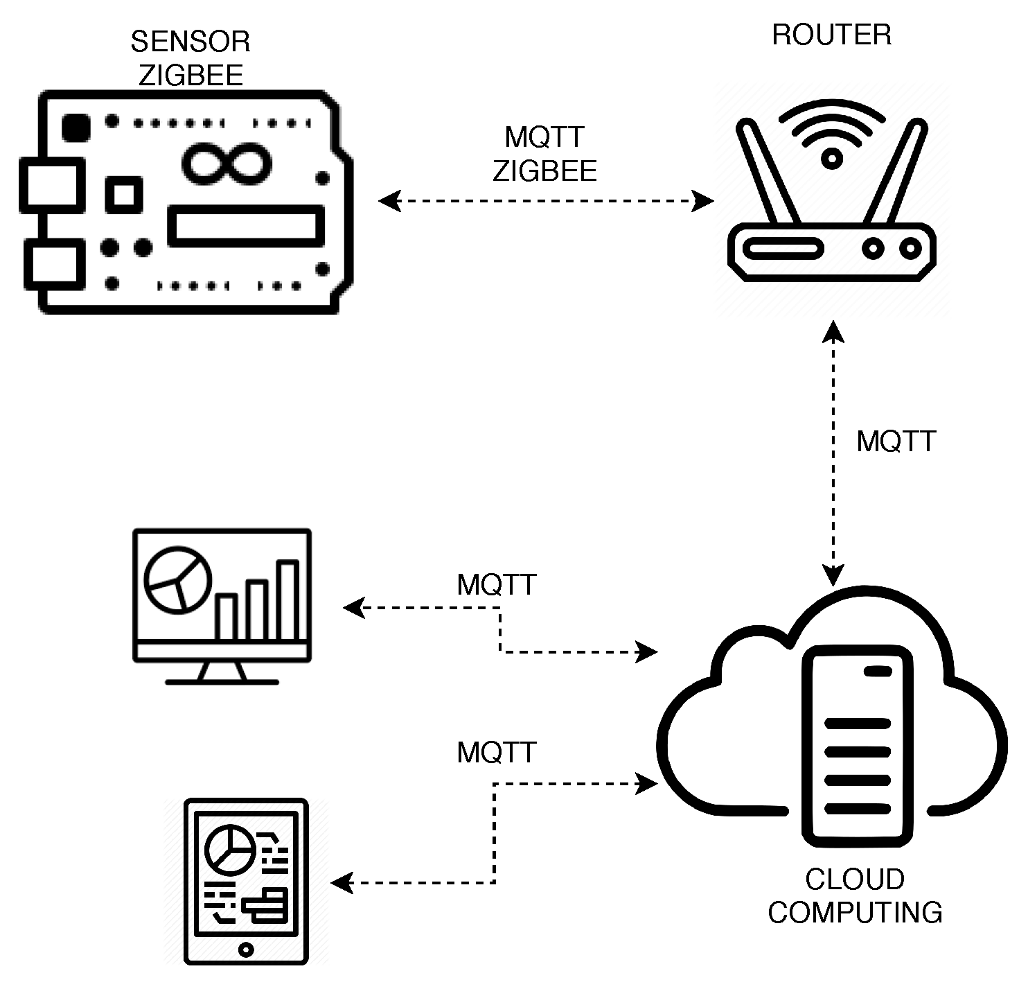
places, it means active and inactive respectively. The failure and repair events for this component are represented by RTR_MTTF and RTR_MTTR transitions, respectively. These transitions also follow a single-server semantic and their firing delays are exponentially distributed. The router on the cloud computing system, which transmits data to the management system, is described by
and
places, indicating active and inactive, respectively. The failure and repair events for this component are represented by RTR_MTTF and RTR_MTTR transitions, respectively. These transitions also follow a single-server semantic and their firing delays are exponentially distributed. The black transitions are immediate, therefore these transitions fire as soon as they are enabled. Equation (
27) expresses the availability of the whole system.
where,
P denotes probability, and # indicates the fraction of tokens in a defined place. Accordingly, the system is available when the central controller (CC), device manager (DM), database (DB), router (RTR), solar power system (PV), smart switch power (SP), and all floors (F) are up. The annual uptime and downtime can be computed using Equations (
28) and (
29), respectively, considering that 8760 corresponds to the number of hours in a year.


