Very Low Sampling Frequency Model Predictive Control for Power Converters in the Medium and High-Power Range Applications

Abstract

Several control strategies have been proposed with the aim to get a desired behavior in the power converter variables. The most employed control techniques are linear control, nonlinear control based on linear and nonlinear feedback, and predictive control. The controllers associated with linear and nonlinear algorithms usually have a fixed switching frequency, featuring a defined spectrum given by the pulse width modulation (PWM) or space vector modulation (SVM) time period. On the other hand, finite set model predictive control (FS-MPC) is known to present a variable switching frequency that results too high for high power applications, increasing losses, reducing the switches lifetime and, therefore, limiting its application. This paper proposes a predictive control approach using a very low sampling frequency, allowing the use of predictive control in high power applications. The proposed method is straightforward to understand, is simple to implement, and can be computed with off-the-shelf digital systems. The main advantage of the proposed control algorithm comes from the combination of the model predictive control and the SVM technique, drawing the principal benefits of both methods. The provided experimental results are satisfactory, displaying the nature of space vector-based schemes but at the same time the fast response as expected in predictive control.

1. Introduction

Controlled power converters have achieved important acceptance to manage voltages and currents. To name a few of the most used topologies out there: (i) back-to-back power converters, which may have different voltage and frequency in their terminals [1,2,3,4]; (ii) unified power quality conditioners (UPQCs), used to minimize the voltage variation at the load, and at the same time, injecting the desired reactive power into the grid supply [5,6]; (iii) STATCOMs to reduce the harmonic distortion and increase the power; (iv) inverters in general as active front end rectifier (AFE), neutral point clamped (NPC), etc., to transform dc to ac energy, used in photovoltaic farms, and motor drives applications [7,8,9]. These topologies have become popular, particularly with the increment of renewable energy penetration into the power grid, which requires more reliable and robust system control in order to maintain the power injection to the distribution grid.

These applications need to be managed by a specific digital controller, which is implemented in discrete time. Among commonly employed controllers are linear [10], nonlinear [11], and predictive [12,13]. Linear and nonlinear control techniques use pulse width modulation (PWM) or space vector modulation (SVM) to switch the power semiconductors, leading to a well-defined switching frequency, which facilitates the passive filter design [14]. On the other hand, conventional model predictive control (MPC), such as Finite-Set MPC (FS-MPC), does not require a PWM or SVM modulator. Indeed, the pulses are selected to reach a given reference through the minimization of a cost function, obtaining a fast dynamic response [3], but with a variable switching frequency.

The main drawback of FS-MPC is the need for a high sampling frequency. In fact, sampling frequencies over 10 kHz are normally reported [15,16,17]. On the other hand, its computational effort increases exponentially as the number of valid power converter states increases, especially in high-power converter topologies. This imposes high requirements over the digital signal processors to implement the algorithm in real-time [18], and specific digital boards are required to compute the entire algorithm in real-time. Furthermore, the fast dynamic imposed by FS-MPC means high switching frequency, and thus precludes its use in high power applications where the losses will be incremented and the efficiency reduced [19,20]. Moreover, the resulting spread spectrum of the electrical variables complicates the passive filtering components design and may generate undesirable resonance problems [21]. Another drawback of FS-MPC is the requirement of appropriate weighting factors when multiple control objectives are desired. In this case, appropriate weighting factors are essential for good performance as they impose the weight of every action or variable. However, their design does not follow a straightforward procedure and usually is a hard task, as it depends upon the cost functions, dynamics, parameters, the weight of every variable in the specific application, and the desired operating point [22].

One of the first approaches to fixed switching frequency in FS-MPC was using virtual state vectors [23]. As the number of converter states is limited, this approach extends this set, generating additional state vectors as linear combinations of them. The problem is that these vectors must be considered in the optimization of the cost function, increasing the computational burden. Instead, Reference [24] proposes to integrate a modulation scheme inside the predictive controller. It does so by predicting the current values for all the available states and calculating equivalent duty cycles for all the corresponding states. The selection is then performed by the minimization of a cost function which depends on their value. However, the method seems cumbersome and not easily extensible for other power converter topologies. An arguably simpler method is proposed in Reference [25], which presents a period control approach to switching frequency regulation in FS-MPC. A new cost function that represents the up and down commutations is added to the total cost function. However, the tuning of the weighting factors is not straightforward. On the other hand, Reference [26] studies the unification of the cost function-based FS-MPC and the deadbeat control-SVM approaches, illustrating the conditions where they are equivalent, based on the tracking of complex power and voltage errors. A unified method is proposed for the PWM rectifier that integrates the previous approaches. However, the results provided show that the spectrum is not totally concentrated as in conventional modulated schemes. Based on this revision, and to the knowledge of the authors, the use of FS-MPC for very low sampling frequency in medium and high-power range applications requires further study.

To address the aforementioned problem, and based on the principle of deadbeat control [26], this paper proposes a model predictive controller in combination with an SVM technique applied to an active front-end rectifier (AFE) achieving reduced switching and sampling frequencies (Figure 1). Moreover, the control technique has the advantages and simplicity of model predictive control, as well as the space vector fixed switching frequency and a well-defined harmonic spectrum. The proposed approach uses the model predictive algorithm to obtain the voltage v_go to be injected by the power converter in order to get a desired current i_g (as in conventional FS-MPC) while the space vector modulator approach synthetizes the voltage v_go by using the closest states. As the required voltage is synthesized by the SVM, the switching frequency is fixed and set by the sampling time of the proposed controller. The proposed controller is simpler than previous approaches, as it does not require performing the optimization process, neither the weighting factors and the hassle of parameters tuning, and has lower computational requirements.

A further advantage of the proposed approach is the low sampling frequency that can be used to control the desired variables. The experimental tests show proper behavior even with only 24 samples per cycle at 50 Hz, i.e., with a 1.2 kHz sampling and switching frequencies, which is a very low sampling frequency when compared with other model predictive control algorithms [2,7,12,13,14,15,16,17,19,27,28]. The ability to sample at very low frequencies makes this strategy an attractive option for multi-cell power converters in high-power range applications, as losses and computational effort are reduced. In fact, just one digital signal processor board with medium to low computational capacity can be used, thus reducing the controller’s complexity, price, and specifications. Although the algorithm is presented in a controlled rectifier application, it is not limited to this configuration. It can be easily extended to other power converters, particularly the ones where the dc link is considered as a constant source, and the currents are imposed by the load needs, as in medium voltage drives.

Experimental results are provided to show the feasibility of the proposed algorithm, to validate the mathematical analysis, and to evaluate the control response. Some of the results include: Fourier spectrum, current control response, dc link voltage reference step changes, and sag/swell responses. All of them show good performance when compared to the conventional approach, despite the use of a very low sampling frequency with respect to the typical values, which range between 20 µs and 100 µs [29,30].

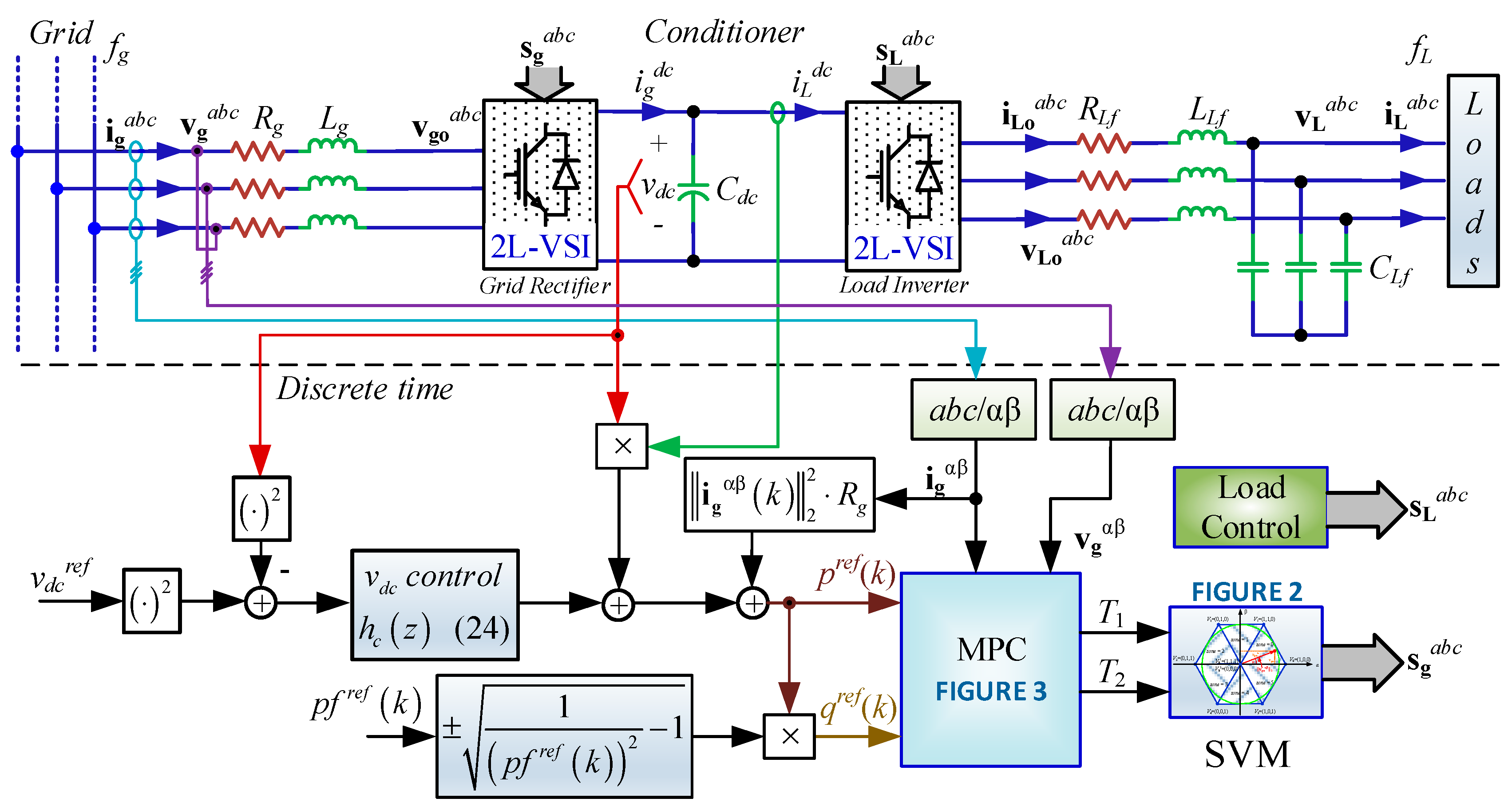
2. Power Converter Model

2.1. Stationary abc Reference Frame Model

The MPC approach needs the mathematical representation of the system. The structure shown in Figure 1 will be considered to illustrate the technique. The grid voltage source v_g is connected throughout a passive RL filter (R_g, L_g) to feed a continuous dc link voltage v_dc. The dc link, constituted by a C_dc capacitor filter, feeds a voltage source inverter (VSI) to supply the load side with a given voltage v_L^abc and frequency f_L. The load neutral point is isolated and a second-order RLC filter is used (R_Lf, L_Lf, C_Lf). The model is found from the Kirchhoff current and voltage laws in a static abc reference frame.

The mathematical representation of the rectifier in Figure 1 using the voltage Kirchhoff’s law is:

$$v_g{}^{abc}=L_g\frac{d{i}_g{}^{abc}}{dt}+R_g{i}_g{}^{abc}+v_{dc}{s}_g{}^{abc}$$

(1)

and the current Kirchhoff’s law to model the dc link capacitor behavior gives:

$$C_{dc}\frac{d{v}_{dc}}{dt}=\langle i_g{}^{abc},s_g{}^{abc}\rangle -i_L{}^{dc}$$

(2)

where $\langle x,y\rangle$ represents the Hadamard product of vectors x and y; s_g^abc and s_L^abc represent the switching state vector of the grid side rectifier and the load side inverter, respectively.

The load side converter can also be modeled through Kirchhoff’s laws, and because of the RLC passive filter, two new equations are included. This work considers the three-phase load current i_L^abc as a disturbance, which depends upon the connected load components, in order to generalize the analysis to any load. Then, the mathematical representation can be written as follows:

$$v_{Lo}{}^{abc}=R_{Lf}{i}_{Lo}{}^{abc}+L_{Lf}\frac{d{i}_{Lo}{}^{abc}}{dt}+v_L{}^{abc}$$

(3)

$$i_{Lo}{}^{abc}=C_{Lf}\frac{d{v}_L{}^{abc}}{dt}+i_L{}^{abc}$$

(4)

where the RLC filter is designed to filter out the commutation harmonics. It is important to highlight that the grid and the load side voltages may have different amplitude, phase, and frequency, and may be controlled independently by decoupled controllers.

2.2. Stationary αβ Reference Frame Model

A stationary αβ reference frame can be employed to reduce the order of the system considering balanced three-phase supply voltages and loads. Furthermore, using only the αβ reference frame allows to implement the control system without a synchronism method, which would be needed by the rotating dq reference frame, improving the dynamic response by avoiding synchronization delays. In fact, the transformation for a particular vector x^abc = [x^a x^b x^c]^T, which can be voltage or current, is applied as:

$${\overrightarrow{x}}^{\mathsf{\alpha }\mathsf{\beta }}=\sqrt{2/3}\left(x^a+\overrightarrow{w}{x}^b+{\overrightarrow{w}}^2{x}^c\right)$$

(5)

where $\overrightarrow{w}=e^{j2\pi /3}$, and the real and imaginary parts of ${\overrightarrow{x}}^{\mathsf{\alpha }\mathsf{\beta }}$ are x^α and x^β, respectively. Then, x^αβ can be rewritten as:

$$x^{\mathsf{\alpha }\mathsf{\beta }}={\left[\begin{array}{cc}\mathrm{Re}\left\{{\stackrel{\rightharpoonup }{x}}^{\mathsf{\alpha }\mathsf{\beta }}\right\}& \mathrm{Im}\left\{{\stackrel{\rightharpoonup }{x}}^{\mathsf{\alpha }\mathsf{\beta }}\right\}\end{array}\right]}^T$$

(6)

Thus, every ac variable of the topology in Figure 1 can be transformed to the αβ reference frame with minor computational effort, and without requiring a synchronization algorithm.

The rectifier model given in Equations (1) and (2) can be transformed to the αβ reference frame leading to:

$$v_g{}^{\mathsf{\alpha }\mathsf{\beta }}=L_g\frac{d{i}_g{}^{\mathsf{\alpha }\mathsf{\beta }}}{dt}+R_g{i}_g{}^{\mathsf{\alpha }\mathsf{\beta }}+v_{go}{}^{\mathsf{\alpha }\mathsf{\beta }}$$

(7)

and for the dc link,

$$C_{dc}\frac{d{v}_{dc}}{dt}=i_g{}^{dc}-i_L{}^{dc}$$

(8)

where:

$$i_g{}^{dc}={\left(s_g{}^{\mathsf{\alpha }\mathsf{\beta }}\right)}^T{i}_g{}^{\mathsf{\alpha }\mathsf{\beta }},i_L{}^{dc}={\left(s_L{}^{\mathsf{\alpha }\mathsf{\beta }}\right)}^T{i}_{Lo}{}^{\mathsf{\alpha }\mathsf{\beta }}$$

(9)

On the other hand, the inverter model given in Equations (3) and (4) of the load side in the αβ reference frame is given by

$$v_{Lo}{}^{\mathsf{\alpha }\mathsf{\beta }}=R_{Lf}{i}_{Lo}{}^{\mathsf{\alpha }\mathsf{\beta }}+L_{Lf}\frac{d{i}_{Lo}{}^{\mathsf{\alpha }\mathsf{\beta }}}{dt}+v_L{}^{\mathsf{\alpha }\mathsf{\beta }}$$

(10)

$$i_{Lo}{}^{\mathsf{\alpha }\mathsf{\beta }}=C_{Lf}\frac{d{v}_L{}^{\mathsf{\alpha }\mathsf{\beta }}}{dt}+i_L{}^{\mathsf{\alpha }\mathsf{\beta }}$$

(11)

2.3. Model Discretization

The MPC needs a discrete model of the system, which is obtained in this work through the Euler approximation of the derivative dx/dt given by:

$$\frac{dx}{dt}\approx \frac{x\left(k+1\right)-x\left(k\right)}{T_s}$$

(12)

where T_s is the controller sampling time. Thus, the αβ rectifier model given in Equations (7) and (11) can be rewritten in a discrete representation. Then, Equation (7) leads to:

$$v_g{}^{\mathsf{\alpha }\mathsf{\beta }}\left(k\right)\approx {\widehat{v}}_g{}^{\mathsf{\alpha }\mathsf{\beta }}\left(k\right)=L_g\frac{i_g{}^{\mathsf{\alpha }\mathsf{\beta }}\left(k+1\right)-i_g{}^{\mathsf{\alpha }\mathsf{\beta }}\left(k\right)}{T_s}+R_g{i}_g{}^{\mathsf{\alpha }\mathsf{\beta }}\left(k\right)+v_{go}{}^{\mathsf{\alpha }\mathsf{\beta }}\left(k\right)$$

(13)

the dc link dynamics (8) is:

$$C_{dc}\frac{v_{dc}\left(k+1\right)-v_{dc}\left(k\right)}{T_s}\approx i_g{}^{dc}\left(k\right)-i_L{}^{dc}\left(k\right)$$

(14)

and the load side, (10) and (11), can be represented by:

$$v_{Lo}{}^{\mathsf{\alpha }\mathsf{\beta }}\left(k\right)\approx {\widehat{v}}_{Lo}{}^{\mathsf{\alpha }\mathsf{\beta }}\left(k\right)=R_{Lf}{i}_{Lo}{}^{\mathsf{\alpha }\mathsf{\beta }}\left(k\right)+L_{Lf}\frac{i_{Lo}{}^{\mathsf{\alpha }\mathsf{\beta }}\left(k+1\right)-i_{Lo}{}^{\mathsf{\alpha }\mathsf{\beta }}\left(k\right)}{T_s}+v_L{}^{\mathsf{\alpha }\mathsf{\beta }}\left(k\right)$$

(15)

$$i_{Lo}{}^{\mathsf{\alpha }\mathsf{\beta }}\left(k\right)\approx {\widehat{i}}_{Lo}{}^{\mathsf{\alpha }\mathsf{\beta }}\left(k\right)=C_{Lf}\frac{v_L{}^{\mathsf{\alpha }\mathsf{\beta }}\left(k+1\right)-v_L{}^{\mathsf{\alpha }\mathsf{\beta }}\left(k\right)}{T_s}+i_L{}^{\mathsf{\alpha }\mathsf{\beta }}\left(k\right)$$

(16)

3. Predictive Control Strategy

3.1. Model Discretization

The rectifier of Figure 1 must ensure a desired dc link voltage by remaining equal to a certain reference. The dc link voltage control can be accomplished in several ways such as linear, nonlinear, and predictive [11,12,13,15,16,17,19,28]. In this paper, the power is controlled to store/release energy into/from the dc link capacitor. The dc link power p_dc can be found from the energy as:

$$\Delta p_{dc}\left(t\right)=d{e}_{dc}\left(t\right)/dt$$

(17)

where the capacitor energy is given by:

$$\Delta e_{dc}\left(t\right)=\left(1/2\right)C_{dc}{v}_{dc}{}^2\left(t\right)$$

(18)

Then, the power is found as:

$$\Delta p_{dc}\left(t\right)=\frac{d{e}_{dc}\left(t\right)}{dt}=\frac{1}{2}{C}_{dc}\frac{d{v}_{dc}{}^2\left(t\right)}{dt}$$

(19)

which shows a linear relationship between the power and the squared dc link voltage. This relationship can be stated in the Laplace s-plane as:

$$h_{Cdc}\left(s\right)=\frac{2}{C_{sc}s}=\frac{v_{dc}{}^2\left(s\right)}{\Delta p_{dc}\left(s\right)}$$

(20)

or in the discrete z-plane as:

$$h_{Cdc}\left(z\right)=\frac{2T_s}{C_{sc}\left(1-z^{-1}\right)}=\frac{v_{dc}{}^2\left(z\right)}{\Delta p_{dc}\left(z\right)}$$

(21)

To regulate the dc link voltage value, a Proportional-Integral (PI) controller is employed to guarantee zero steady-state error to compensate for parasitic components associated with the dc link capacitor. Its transfer function is given by:

$$h_c\left(z\right)=k_c\frac{\left(1+T_s/2T_i\right)+\left(-1+T_s/2T_i\right)z^{-1}}{1-z^{-1}}$$

(22)

where T_s, k_c, T_i are the sampling time, the PI gain, and the integrative time, respectively. The output of the PI controller is the instantaneous power required from the supply:

$$p_{Cdc}\left(k\right)=p_{Cdc}\left(k-1\right)+k_c\left[\left(1+\frac{T_s}{2T_i}\right)e\left(k\right)+\left(-1+\frac{T_s}{2T_i}\right)e\left(k-1\right)\right]$$

(23)

The corresponding active current reference can be written as:

$${i_g}^{\mathsf{\alpha }\mathsf{\beta },ref}\left(k\right)=\left[\begin{array}{c}{i_g}^{\mathsf{\alpha },ref}\left(k\right)\\ {i_g}^{\mathsf{\beta },ref}\left(k\right)\end{array}\right]=\frac{1}{{\Vert v_g{}^{\mathsf{\alpha }\mathsf{\beta }}\left(k\right)\Vert }_2^2}\left[\begin{array}{c}\mathrm{Re}\left\{{\overrightarrow{s}}_{pq}{{}^{ref}}^{*}\left(k\right)\cdot {\overrightarrow{v}}_g{}^{\mathsf{\alpha }\mathsf{\beta }}\left(k\right)\right\}\\ \mathrm{Im}\left\{{\overrightarrow{s}}_{pq}{{}^{ref}}^{*}\left(k\right)\cdot {\overrightarrow{v}}_g{}^{\mathsf{\alpha }\mathsf{\beta }}\left(k\right)\right\}\end{array}\right]$$

(24)

where $\Vert \cdot \Vert$₂ represents the 2-norm, ${\overrightarrow{x}}^{*}$ means $\overrightarrow{x}$ conjugate, and ${\overrightarrow{s}}_{pq}{}^{ref}\left(k\right)$ is the apparent power defined as:

$${\overrightarrow{s}}_{pq}{}^{ref}\left(k\right)=\left({\Vert i_g{}^{\mathsf{\alpha }\mathsf{\beta }}\left(k\right)\Vert }_2^2{R}_g+p_{Cdc}\left(k\right)+v_{dc}\left(k\right)i_L^{dc}\left(k\right)\right)\left(1\pm j\sqrt{\frac{1}{{\left(p{f}^{ref}\left(k\right)\right)}^2}-1}\right)=p^{ref}\left(k\right)+j{q}^{ref}\left(k\right)$$

(25)

with $p{f}^{ref}\left(k\right)$ the power factor reference. It is important to highlight that the power control is mainly dominated by the dc capacitor dynamic, and it must be tuned to be slower than the inner current control loop, to decouple both controllers. Ten times slower can be used as a guideline [31].

3.2. Rectifier Injected Voltage

Since the grid voltage v_g^abc is measurable, then to get a desired grid current i_g^abc, the applied voltage v_go^abc must be controlled to reach the current reference (24) or power reference (25) (Figure 1). In order to achieve the current reference given in (24), the following control strategy is designed.

From (13), a prediction of the future current value $i_g{}^{\mathsf{\alpha }\mathsf{\beta }}\left(k+1\right)$ can be found as:

$$i_g{}^{\mathsf{\alpha }\mathsf{\beta }}\left(k+1\right)\approx {\widehat{i}}_g{}^{\mathsf{\alpha }\mathsf{\beta }}\left(k+1\right)=\left(1-\left(T_s{R}_g/L_g\right)\right)i_g{}^{\mathsf{\alpha }\mathsf{\beta }}\left(k\right)+\left(T_s/L_g\right)\left(v_g{}^{\mathsf{\alpha }\mathsf{\beta }}\left(k\right)-v_{go}{}^{\mathsf{\alpha }\mathsf{\beta }}\left(k\right)\right)$$

(26)

Equation (26) can be computed in real-time because i_g^αβ(k) and v_g^αβ(k) are measured at the instant k, and v_go^αβ(k) is known since this voltage is predicted beforehand, as explained later. In addition, from (13), the voltage to be applied at k + 1 v_go^αβ(k + 1) can be found as:

$$v_{go}{}^{\mathsf{\alpha }\mathsf{\beta }}\left(k+1\right)={\widehat{v}}_g{}^{\mathsf{\alpha }\mathsf{\beta }}\left(k+1\right)-R_g{\widehat{i}}_g{}^{\mathsf{\alpha }\mathsf{\beta }}\left(k+1\right)-\frac{L_g}{T_s}\left(i_g{}^{\mathsf{\alpha }\mathsf{\beta }}\left(k+2\right)-{\widehat{i}}_g{}^{\mathsf{\alpha }\mathsf{\beta }}\left(k+1\right)\right)$$

(27)

where ${\widehat{i}}_g{}^{\mathsf{\alpha }\mathsf{\beta }}\left(k+1\right)$ comes from (26), and $i_g{}^{\mathsf{\alpha }\mathsf{\beta }}\left(k+2\right)$ can be set as the current reference $i_g{}^{\mathsf{\alpha }\mathsf{\beta },ref}\left(k+2\right)$. As the reference in (24) is set at time k, then the Euler extrapolation is given by:

$${\overrightarrow{\widehat{i}}}_g{}^{\mathsf{\alpha }\mathsf{\beta },ref}\left(k+2\right)\approx {\overrightarrow{\widehat{i}}}_g{}^{\mathsf{\alpha }\mathsf{\beta },ref}\left(k\right)e^{j2\Delta \mathsf{\theta }}={\overrightarrow{\widehat{i}}}_g{}^{\mathsf{\alpha }\mathsf{\beta },ref}\left(k\right)e^{j2\mathsf{\omega }{T}_s}$$

(28)

where employing (24):

$$i_g{{}^{\mathsf{\alpha }\mathsf{\beta }}}^{,}{}^{ref}\left(k+2\right)=\left[\begin{array}{l}{i}_g{}^{\mathsf{\alpha },ref}\left(k\right)\cos \left(2\mathsf{\omega }{T}_s\right)-i_g{}^{\mathsf{\beta },ref}\left(k\right)\sin \left(2\mathsf{\omega }{T}_s\right)\\ i_g{}^{\mathsf{\alpha },ref}\left(k\right)\sin \left(2\mathsf{\omega }{T}_s\right)+i_g{}^{\mathsf{\beta },ref}\left(k\right)\cos \left(2\mathsf{\omega }{T}_s\right)\end{array}\right]$$

(29)

Likewise, the voltage $\widehat{v}$_g^αβ(k + 1) can be obtained from the same extrapolation as:

$${\widehat{\overrightarrow{v}}}_g{}^{\mathsf{\alpha }\mathsf{\beta }}\left(k+1\right)\approx {\overrightarrow{v}}_g{}^{\mathsf{\alpha }\mathsf{\beta }}\left(k\right)e^{j\Delta \mathsf{\theta }}={\overrightarrow{v}}_g{}^{\mathsf{\alpha }\mathsf{\beta }}\left(k\right)e^{j\mathsf{\omega }{T}_s}$$

(30)

and (6) becomes:

$${\widehat{v}}_g{}^{\mathsf{\alpha }\mathsf{\beta }}\left(k+1\right)=\left[\begin{array}{l}{v}_g{}^{\mathsf{\alpha }}\left(k\right)\cos \left(\mathsf{\omega }{T}_s\right)-v_g{}^{\mathsf{\beta }}\left(k\right)\sin \left(\mathsf{\omega }{T}_s\right)\\ v_g{}^{\mathsf{\alpha }}\left(k\right)\sin \left(\mathsf{\omega }{T}_s\right)+v_g{}^{\mathsf{\beta }}\left(k\right)\cos \left(\mathsf{\omega }{T}_s\right)\end{array}\right]$$

(31)

where $\sin \left(\mathsf{\omega }{T}_s\right)$ and $\cos \left(\mathsf{\omega }{T}_s\right)$ are constant values, and ω is the system frequency in rad/s. Note that $\widehat{v}$_g^αβ(k + 1) may be different from v_g^αβ(k + 1), and they are equal only if the amplitude and frequency remain constant. However, if the frequency and amplitude are close enough to constant values, the approximation given by (31) shows to be accurate. Furthermore, because the sampling frequency on this approach may be very low, and just a few points per cycle are available, the difference between v_g^αβ(k + 1) and v_g^αβ(k) may become important. This means that the usual approximation v_g^αβ(k + 1) ≈ v_g^αβ(k) cannot be used in this context.

The previous results show the voltage v_go^αβ in (27) as the voltage necessary to obtain a given current value at k + 2. This voltage needs to be synthesized, which is performed by means of the SVM technique.

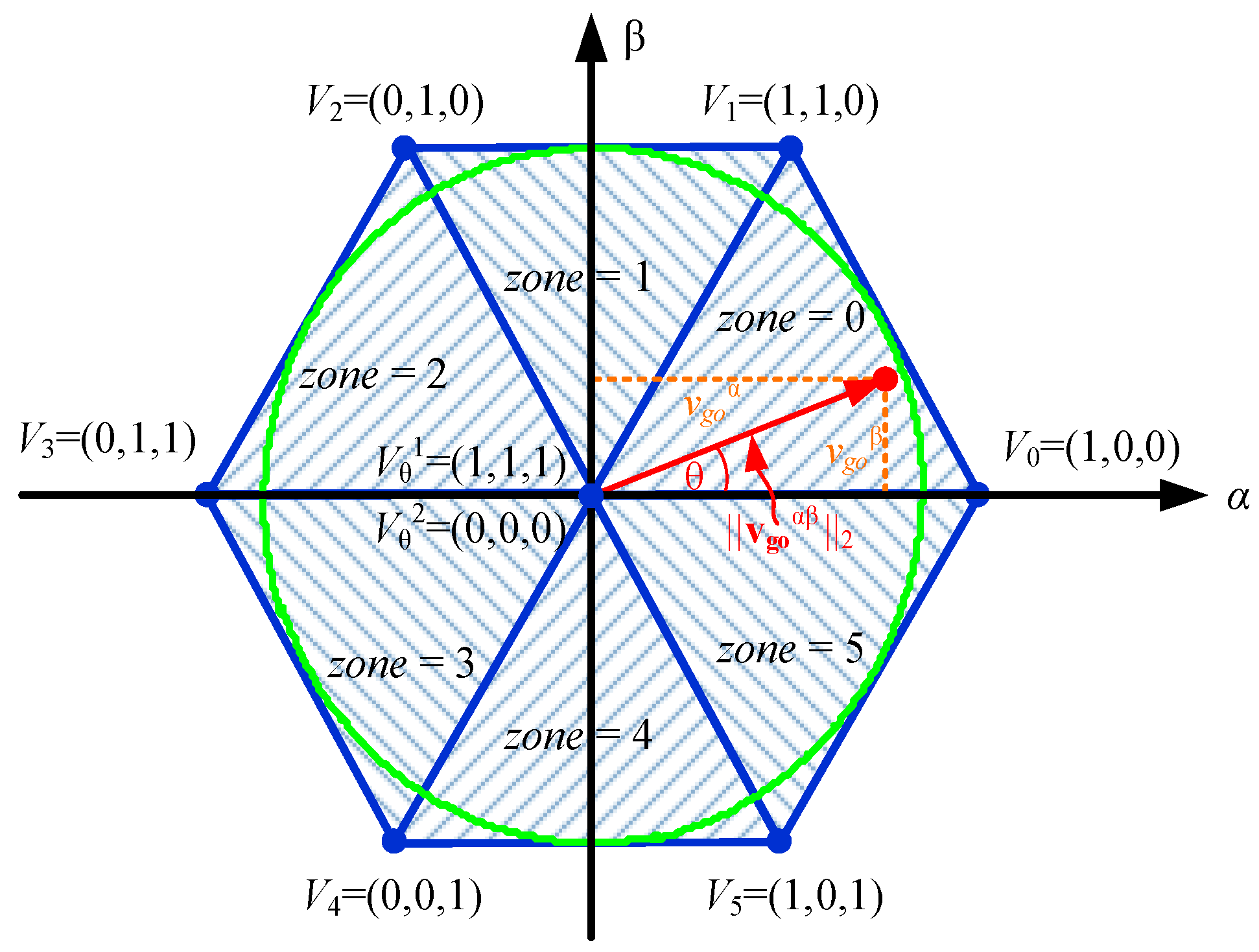
3.3. Required Voltage Based on Space Vector

The desired voltage in (27) cannot be implemented directly because it may contain just the fundamental value, which is different from the valid states, Figure 2. Thus, the SVM technique can be employed to synthesize the desired voltage value v_go^αβ of (27).

The voltage v_go^αβ can be in any zone {0, 1, 2, 3, 4, 5}, described in the complex plane of Figure 2, where a 2-level VSI is considered. The vector v_go^αβ in red (Figure 2) shows one possible value highlighting the v_go^α and v_go^β components. The voltage v_go^αβ with angle θ determines the zone and the closest three states. Thus, the zone can be defined as a function of θ(k + 1) as:

$$\begin{array}{ll}\mathrm{if}\left(0\le \mathsf{\theta }\left(k+1\right)<\pi /3\right),& \mathrm{then}\hspace{1em}\hspace{1em}zone=0\\ \mathrm{if}\left(\pi /3\le \mathsf{\theta }\left(k+1\right)<2\pi /3\right),& \mathrm{then}\hspace{1em}\hspace{1em}zone=1\\ \mathrm{if}\left(2\pi /3\le \mathsf{\theta }\left(k+1\right)<\pi \right),& \mathrm{then}\hspace{1em}\hspace{1em}zone=2\\ \mathrm{if}\left(-\pi \le \mathsf{\theta }\left(k+1\right)<-2\pi /3\right),& \mathrm{then}\hspace{1em}\hspace{1em}zone=3\\ \mathrm{if}\left(-2\pi /3\le \mathsf{\theta }\left(k+1\right)<-\pi /3\right),& \mathrm{then}\hspace{1em}\hspace{1em}zone=4\\ \mathrm{if}\left(-\pi /3\le \mathsf{\theta }\left(k+1\right)<0\right),& \mathrm{then}\hspace{1em}\hspace{1em}zone=5\end{array}$$

(32)

Meanwhile, the angle θ(k + 1) is given by:

$$\mathsf{\theta }\left(k+1\right)=\arg \left\{v_{go}{}^{\mathsf{\alpha }\mathsf{\beta }}\left(k+1\right)\right\}=\mathrm{sign}\left(v_{go}{}^{\mathsf{\beta }}\left(k+1\right)\right)\cdot \arccos \left(\frac{v_{go}{}^{\mathsf{\alpha }}\left(k+1\right)}{{\Vert v_{go}{}^{\mathsf{\alpha }\mathsf{\beta }}\left(k+1\right)\Vert }_2}\right)$$

(33)

Once the angle is computed then any voltage v_go^αβ inside the hatched area in Figure 2 can be attained as a linear combination of the three nearest vectors V_zone, V_{zone + 1} and V_θ. This voltage synthesization, for a given zone of the voltage v_go^αβ, can be formed using the following equality (Figure 2):

$$T_s{v}_{go}{}^{\mathsf{\alpha }\mathsf{\beta }}=V_{zone}{}^{\mathsf{\alpha }\mathsf{\beta }}{v}_{dc}{T}_1+V_{zone+1}{}^{\mathsf{\alpha }\mathsf{\beta }}{v}_{dc}{T}_2+V_{\mathsf{\theta }}{}^{\mathsf{\alpha }\mathsf{\beta }}\left(T_s-T_1-T_2\right)$$

(34)

where the vector V_zone^αβ is applied for T₁ time units, V_{zone + 1}^αβ for T₂ time units, and the zero vector V_θ^αβ for the rest of the time to complete the sampling time T_s, and where v_dc is the dc link voltage. The solution of (34) is given by:

$$T_1=\frac{\left(v_{dc}{V}_{zone+1}{}^{\mathsf{\alpha }\mathsf{\beta }}\right)\times v_{go}{}^{\mathsf{\alpha }\mathsf{\beta }}}{\left(v_{dc}{V}_{zone+1}{}^{\mathsf{\alpha }\mathsf{\beta }}\right)\times \left(v_{dc}{V}_{zone}{}^{\mathsf{\alpha }\mathsf{\beta }}\right)}{T}_s$$

(35)

$$T_2=\frac{v_{go}{}^{\mathsf{\alpha }}}{v_{dc}{V}_{zone+1}{}^{\mathsf{\alpha }}}{T}_s-\frac{v_{dc}{V}_{zone}{}^{\mathsf{\alpha }}}{v_{dc}{V}_{zone+1}{}^{\mathsf{\alpha }}}{T}_1$$

(36)

where T₁ and T₂ should be into the interval [0 T_s]; and V_zone^αβ is defined as:

$$V_{zone}{}^{\mathsf{\alpha }\mathsf{\beta }}=\sqrt{\frac{2}{3}}\left[\begin{array}{l}\cos \left(zone\cdot \pi /3\right)\\ \sin \left(zone\cdot \pi /3\right)\end{array}\right]$$

(37)

From (34), the zero state can be either V_θ¹ or V_θ² (because there are two zero states) resulting in the same v_go^αβ, i.e., null voltage. However, in order to minimize the switching, the zero states will be selected to change only one switch at a time, thus:

$$\begin{array}{ll}\mathrm{if}\left(zone\mathrm{is}\mathrm{even}\right),\mathrm{then}& V_{\mathsf{\theta }}{}^1={\left[\begin{array}{ccc}1& 1& 1\end{array}\right]}^T\\ \mathrm{if}\left(zone\mathrm{is}\mathrm{odd}\right),\mathrm{then}& V_{\mathsf{\theta }}{}^2={\left[\begin{array}{ccc}0& 0& 0\end{array}\right]}^T\end{array}$$

(38)

and only one switch changes its state from V_zone^αβ to V_{zone + 1}^αβ.

Figure 3 summarizes the control algorithm, highlighting all the steps to find the times T₁ and T₂. The diagram in Figure 3 shows a simple algorithm employed and how to implement it in a digital system. In addition, the previous procedure does not need the tuning of any parameter, does not require synchronization as it uses a stationary frame, and the dynamic response will always be the fastest for the chosen sampling time since this controller chooses the shortest path to the reference [30]. As expected, the only limitation of the response is related to the dc link voltage v_dc and the input RL filter size, as in any other control approach.

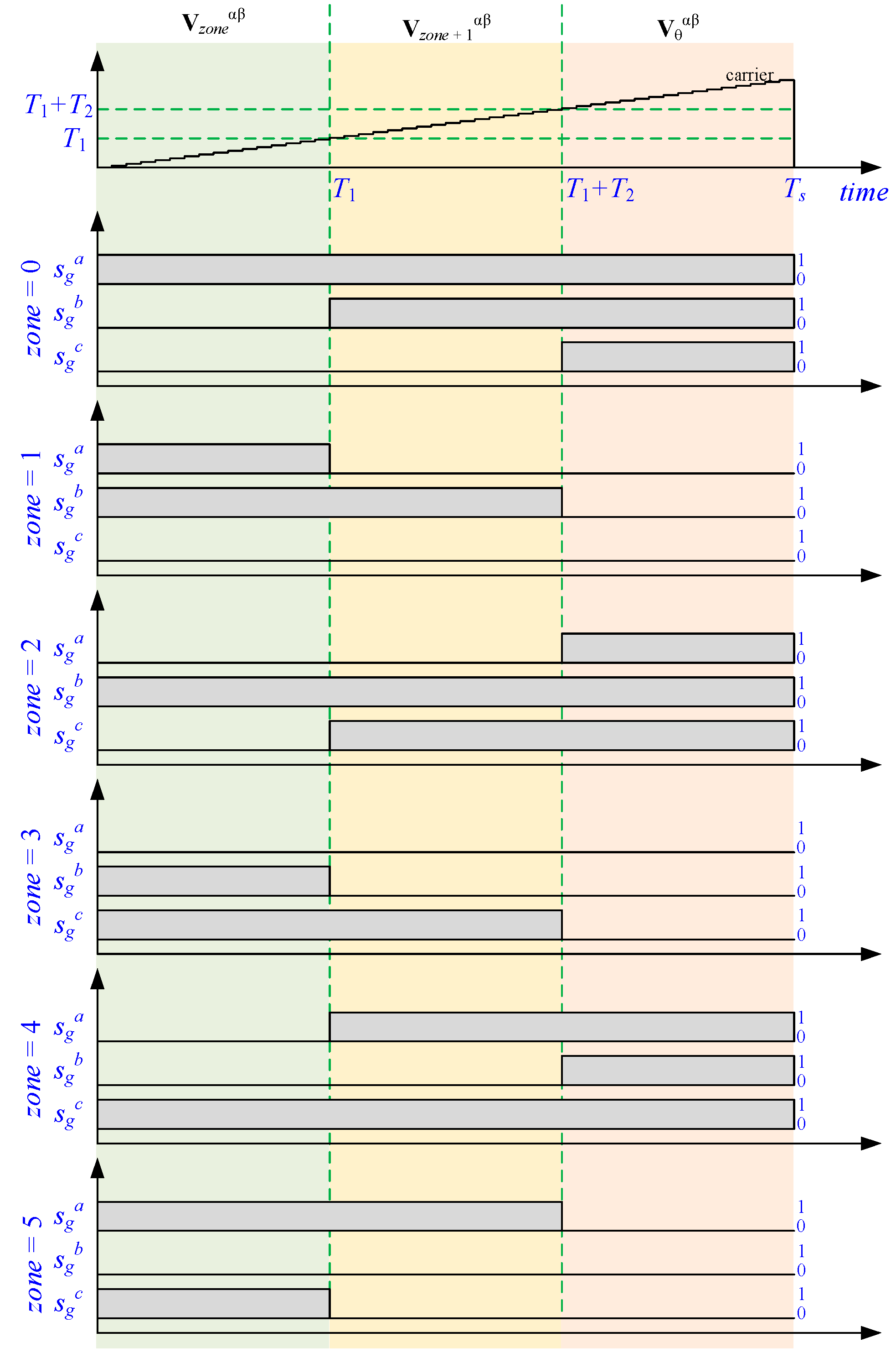
3.4. Switching Generation for a PWM Implementation

The PWM technique is used to generate gating pulses. Figure 4 shows the count-up carrier used to compare with times T₁ and T₁ + T₂ as defined by (35) and (36). The counter should increase its value up to T_s and then needs to be reset. The comparison indicates when to switch on, switch off, or do nothing for every insulated-gate bipolar transistor (IGBT) (S_g^a, S_g^b, S_g^c) of the rectifier in Figure 1. The PWM module only needs to include a count-up counter and three comparators for T₁ and T₁ + T₂. In addition, Figure 4 shows the pattern the IGBT will follow in order to impose the three nearest voltages V_zone^αβ, V_{zone + 1}^αβ V_θ^αβ, following the counterclockwise direction. In addition, Figure 4 shows the waveform patterns depending upon the zone given by the angle θ (32) to get the required voltage (27) necessary to track the current reference (24).

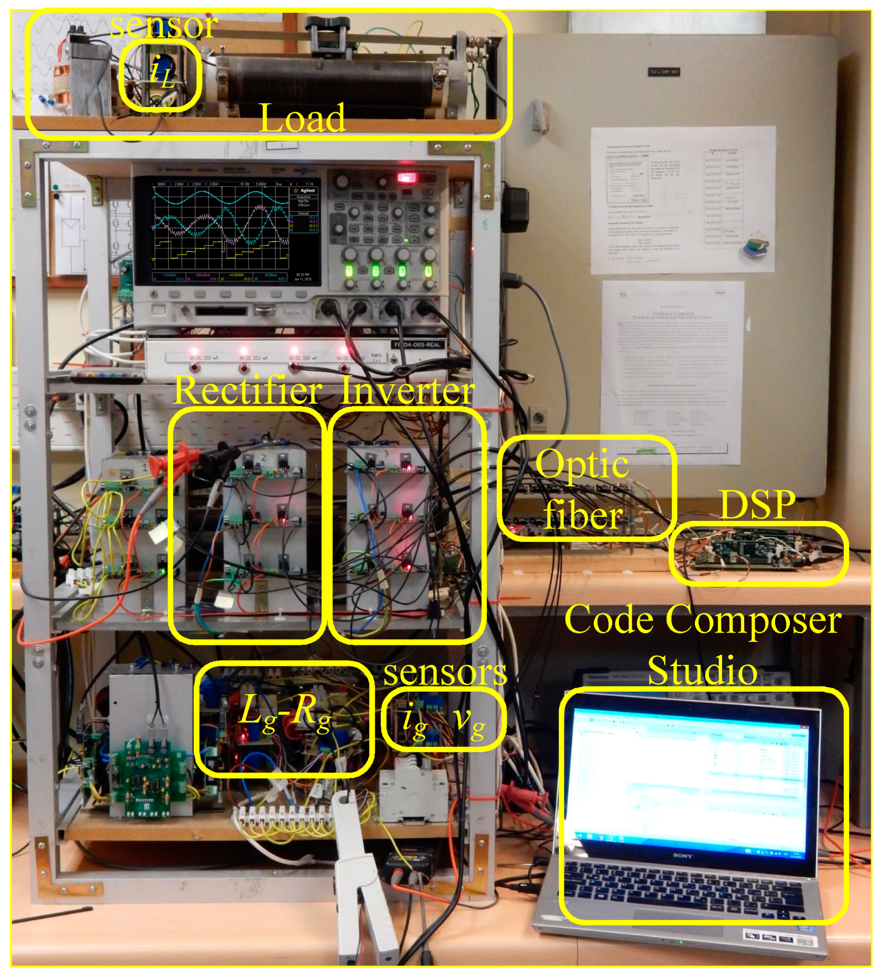
4. Materials and Methods

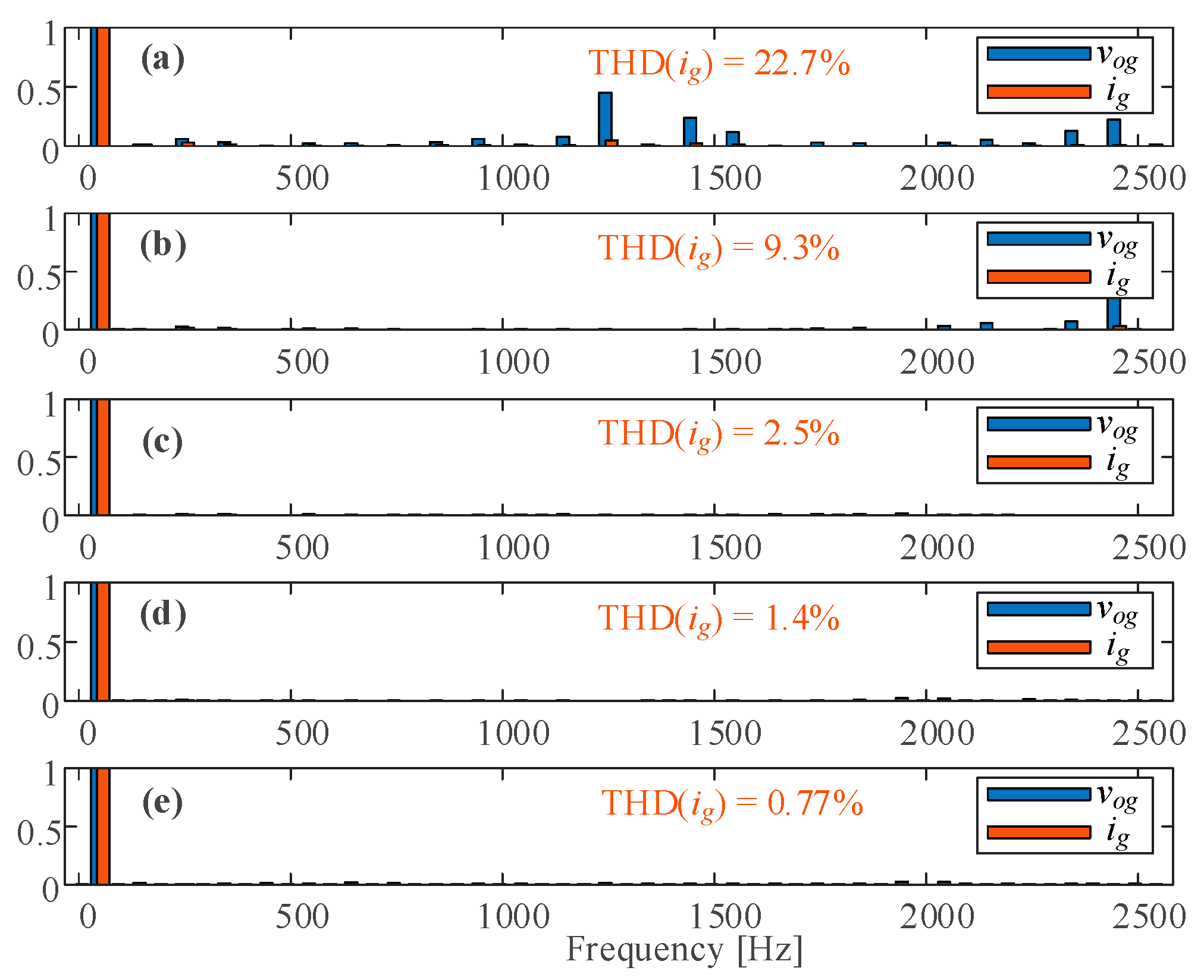
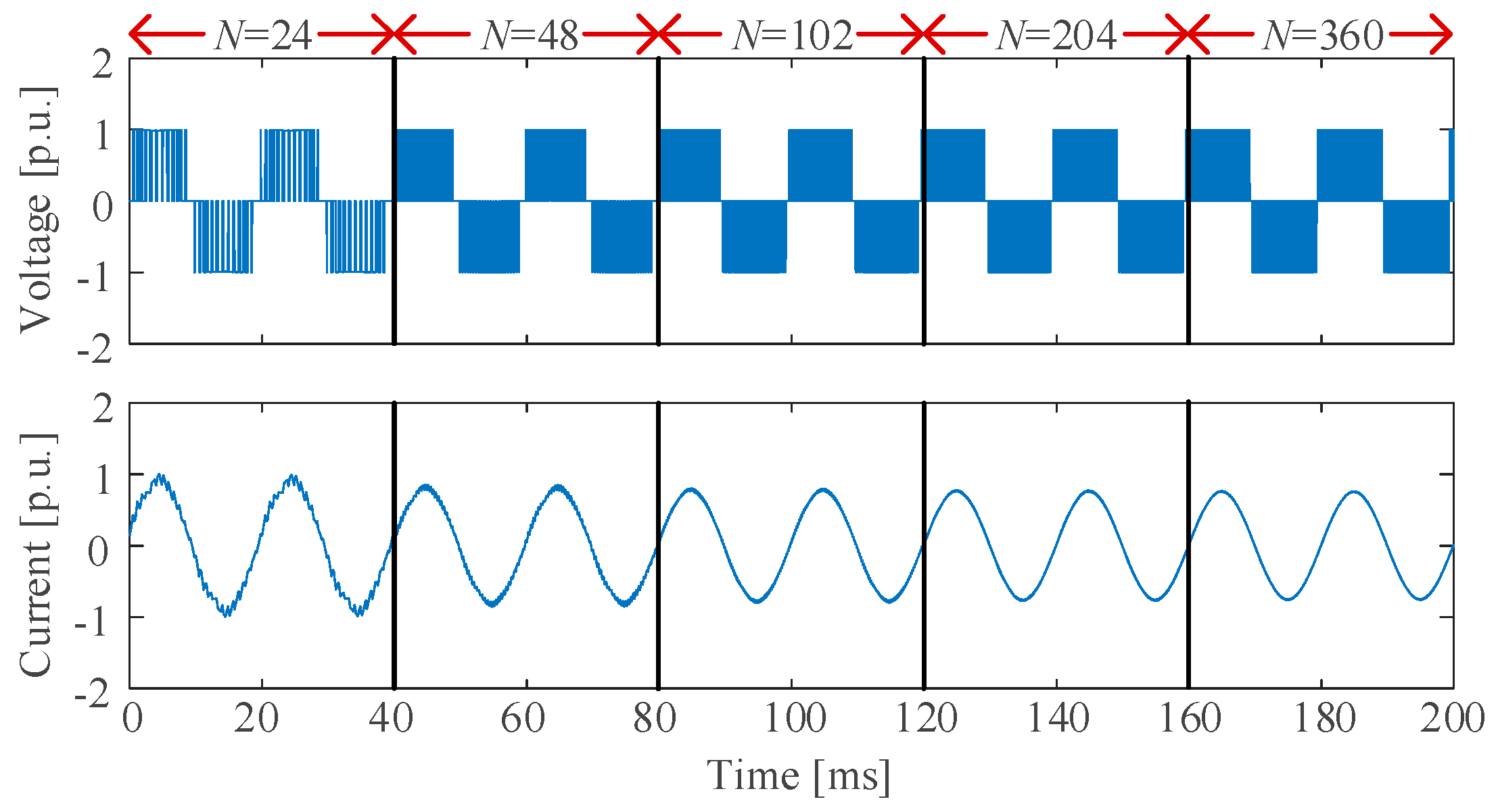
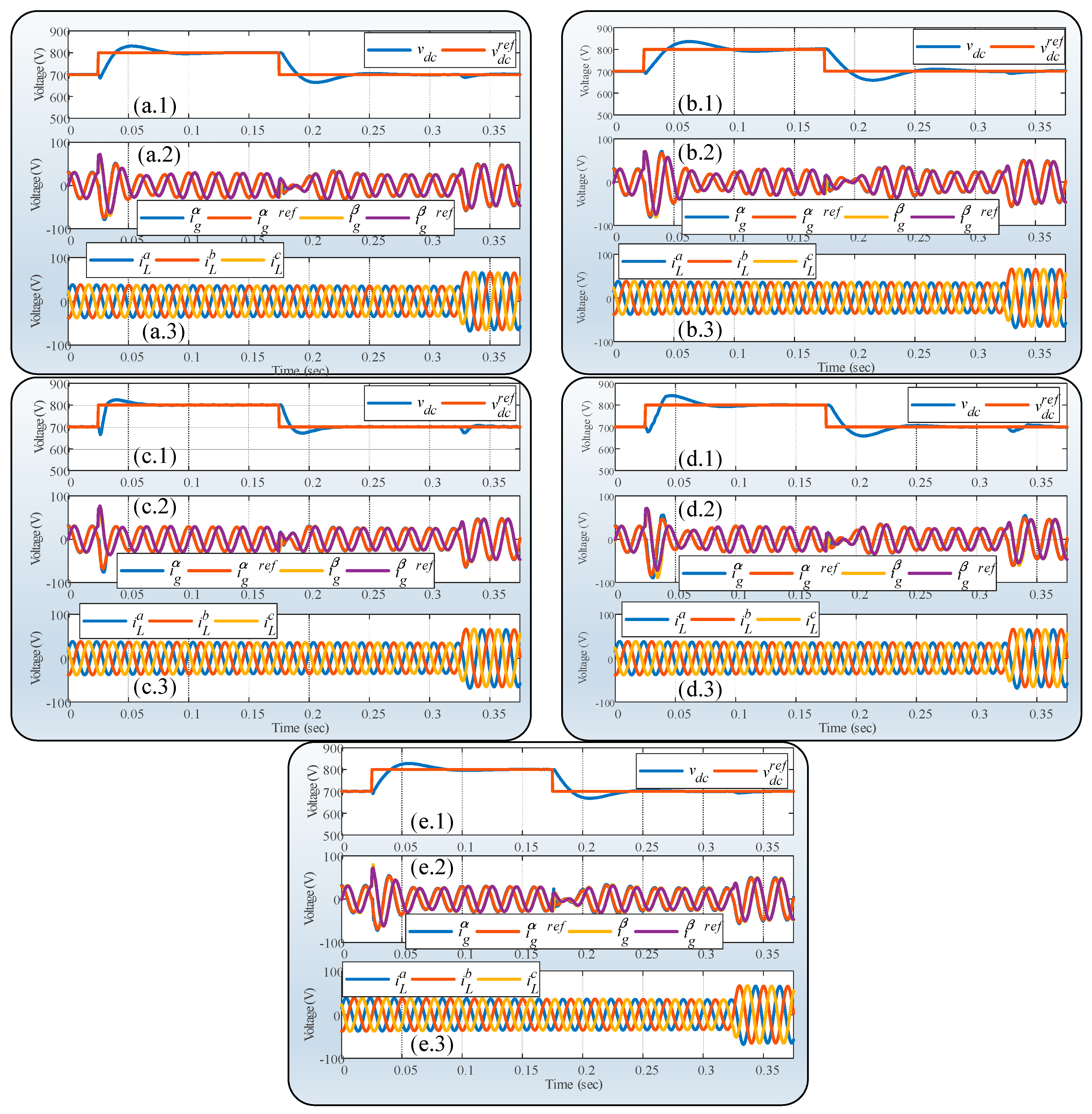
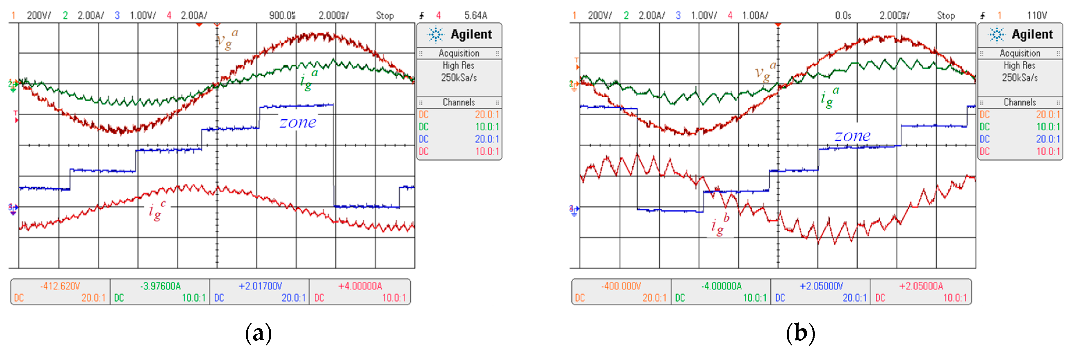
A laboratory prototype setup is used to verify the proposed control (Figure 5). Both the rectifier and the inverter have three legs, with two IGBTs each one, the six legs are identically designed, and use the IGBT 726-IKW20N65ET7XKSA1. The control is carried out in a TMS320F28335 DSP system board, which receives the sensed signals, computes the algorithm code, and generates the pulses for the IGBTs. The sensors used to measure currents are LEM LA 55P, and LEM LV 25P to measure voltages; both sensors generate a current proportional to the measurement, which is then transformed into voltage in a range of 0 (V) to 3.3 (V) (according to the ADC operating range). In order to minimize the induced noise in the IGBTs pulses, the electrical pulses generated by the DSP are transformed into light pulses and sent to the converter by optical fiber. Finally, in order to set the references in the DSP, the Code Composer Studio (CCS) software is employed in the laptop. Several tests are performed in the prototype in order to validate the theoretical results. All the tests will be presented in the Experimental Results section.

5. Results

In order to verify the theoretical developments, emphasize the appeal of the proposal, and to study how the technique can operate with low-switching frequency as well as in high power converters, several tests are performed in simulations and in a laboratory prototype. The parameters employed for the tests are listed in

Table 1. Parameters.

Parameters	Value	P.U.
vg	220 V, rms	1
ZL	8.8 Ω	1
RL—LL	7 Ω—17 mH	0.80—0.61
Rg—Lg	0.4 Ω—12 mH	0.011—0.43
Cdc	2.35 mF	0.677
RLf—LLf—CLf	1 mΩ—3 mH—10 μF	0.12 m 0.36 m—3.183
fg—fL	50 Hz—50 Hz	1
fs	1.2 kHz	24

.

5.1. Simulated Results

The advantage of the proposed method is to reduce the sampling frequency and, therefore, allowing to work with higher power and with lower switching losses. To quantify its performance, Figure 6 shows the harmonic contents and the total harmonic distortion (THD) considering different sampling frequencies the proposed control may use, from 1.2 kHz up to 18 kHz, where the switching frequency is f_s = N∙f_g. The voltage and current waveforms corresponding to the same frequencies of Figure 6 are shown in Figure 7. As can be observed, the higher the sampling frequency, the better the current and voltage waveforms. This is to be expected, as the filter was designed for the worst-case condition.

When the THD needs to be kept constant for a reduced N, the filter needs to be redesigned properly according to the required THD. This can be done considering that the gain G (h) as a function of every harmonic h is:

$$G\left(h\right)={\left(\sqrt{R_g{}^2+{10}^4{\pi }^2{h}^2{L}_g{}^2}\right)}^{-1}$$

(39)

From this equation, the required RL parameters can be found according to the desired maximum THD [32] and the results from Figure 6 and Figure 7.

Particularly, the THD for N = 24 and N = 48 do not fit the standards (as the IEEE 519 and IEEE 1547) for the parameters considered, which recommend a THD less than 5% for grid currents [33]. However, as this paper presents a predictive controller with low switching and sampling time to extend the model predictive control strategy to higher power ranges, this THD is compared with the ones generated by diode and thyristor bridges, where the THD is higher and lower frequency harmonics (5th, 7th, 11th, 13th, etc.) are present, which are more difficult to eliminate. Despite the aforementioned, the THD in the proposed topology can be reduced by employing two well-known techniques: (i) passive filters, which are less bulky, in this case, because the harmonics to be eliminated are at higher frequencies (1200 Hz for N = 24, 2400 Hz for N = 48, and so on) as compared with the ones generated by diode and thyristor bridges (ii) increasing the ac inductive filter L_g, in fact, if the inductance is increased to 20 mH, the THD is reduced to 5% for N = 24, matching the standard requirements, although the penalty is a slower dynamic because of the larger inductor.

Parameter variations are part of practical implementations, for instance, commercial resistors and inductors usually have a 20% tolerance. Therefore, it is expected to have such variations. Figure 8 shows the power converter control response under parameters variation. It is important to highlight that only the parameters in the power converter are changed, and the parameters in the controller are kept as the ones listed in Table 1. Figure 8a shows the performance under nominal conditions. Then, Figure 8b shows the result when increasing the dc capacitor 50%, where it is easy to note that because of this change the dc voltage control dynamic becomes slower. On the contrary, Figure 8c shows a decrease in C_dc, where in this case, the control response is faster because the energy storage (C_dc) is reduced and, therefore, less energy is needed to change the voltage. Figure 8d shows a 50% increase in the coupling inductance, where both controllers, αβ current and dc voltage, are almost unaffected by this parameter change. Additionally, if the inductance is reduced to 50%, Figure 8e, the same conclusion can be drawn.

5.2. Experimental Results

To verify the mathematical analysis, a prototype of the topology shown in Figure 1 runs the proposed approach in a TMS320F28335 DSP board. A California Instruments Programmable CSW5550 Power Source is used to provide and manage the grid amplitude and frequency. The results are acquired using the parameters of Table 1 using a f_s = 1.2 kHz, which is a very low sampling time for this class of predictive control algorithms.

As mentioned before, the switching frequency is fixed and defined by the sampling time T_s. This can be certainly seen in Figure 9 where two different sampling times are employed. Figure 9a shows N = 48 samples per cycle, or f_s = 2.4 kHz, and where the switching frequency is highlighted on the screenshot. Besides, Figure 9b shows N = 24 samples per cycle, or f_s = 1.2 kHz. As before, the switching frequency is defined by the sampling frequency, which is highlighted on the graphic. The results of Figure 9 show a very high sampling time close to 1 ms. This sampling time means that cheaper digital boards can be employed to control this power converter. It also justifies the proposal that only one digital board can be employed to control various power converters simultaneously, not only for high power applications but also when a budget reduction is required.

Another important subject is that every switch changes at most once in any carrier period, and in every event (at T₁ or T₂), just one switch changes its state, reducing the commutation losses and improving the distribution of the thermal stresses among the different switches, as seen in Figure 4. This makes the approach suitable for high current power converter applications. As the SVM is programmed to be completed in one period, Figure 4, the switching frequency is equal to the sampling frequency, as previously mentioned. Figure 9 shows the Fourier transform of the PWM voltage v_go, which is directly related to the sampling frequency. Figure 10 shows one period to highlight the zones given by (32) in order to get the desired voltage v_go^αβ. The current ripple shows a low switching frequency, for Figure 10a is 2.4 kHz and for Figure 10b 1.2 kHz.

To complete the study, tests are performed for the entire control system, to see the response under references and disturbances changes. The current control step response test is shown in Figure 11, where the results show a fast-dynamic response, typical of predictive control, but without increasing the switching frequency, which remains constant at just 1.2 kHz. Figure 12a shows a step-up change in the v_dc voltage control reference, where the experimental results show good behavior and a fast-current response in order to reach the new reference value. Figure 12b shows a step-down change in the v_dc voltage reference. As for the step-up test, the current control shows an accurate response in order to reach the required power to keep the dc voltage at the desired value. Figure 12c shows a sag disturbance on the grid voltage. After the event occurs, it can be seen that the grid currents i_g^a and i_g^b increase their values in order to regulate the desired dc link voltage. The dc link voltage quickly reaches its reference even under a 30% sag event. On the other hand, Figure 12d shows a swell of 30% on the grid voltage v_g, and despite the low sampling frequency, the dc link voltage control and the current control show an accurate response.

6. Discussion

The results show that the MPC proposal based on the dead-beat control principle in combination with SVM has a good behavior suitable for high-power applications under low switching frequency. This is confirmed in both simulations and experimental evaluations considering a low switching frequency of just 1.2 kHz in a 50 Hz system. It was confirmed that the MPC application is feasible for low-frequency applications, capturing the main advantages of this type of control: fast response and simple implementation. The findings indicate that the incorporation of SVM provides the dominant harmonic frequency of the current to be concentrated at the sampling frequency, which facilitates the design of the passive harmonic filters.

The experimental application highlights the presence of relevant harmonic content when low switching frequencies are used. Compared to conventional schemes (diode and thyristor bridges), this proposal has important advantages by requiring smaller passive filters with lower costs since it has a lower THD and presents higher harmonic frequencies (from the 24th harmonic in the proposal and from the 3rd or 5th harmonic in the conventional schemes). Even so, the resulting current THD is high and exceeds the threshold set in the IEEE 519 and IEEE 1547 standards. This requirement can be addressed in future research studies that design a converter filter that ensures fast current dynamic and achieves an adequate THD, avoiding the incorporation of additional passive filters as in conventional solutions.

In addition, since the experimental platform is performed in a scaled-down laboratory, in future research studies a higher power converter structures could be implemented. This would corroborate that this hybrid technique reduces the harmonic content when using multilevel structures by increasing the equivalent dominant harmonic frequency while maintaining the switching frequency of each switch. Moreover, at high power, a substantial increase in the computational effort would not be generated since the proposed MPC is not based on optimization but on the dead-beat control principle.

7. Conclusions

A control strategy for static power converters that combines an MPC and a space vector modulator approach suitable for high power applications has been proposed. The resulting algorithm combines the advantages of both alternatives, (i) it is straightforward to be implemented in digital-based systems, (ii) it features a fast dynamic response, (iii) it can be used at the low switching frequency, (iv) the harmonics are concentrated at well-known frequencies, (v) it can be used with high sampling times, and (vi) it does not present the hassle of parameter selection. The proposed approach uses a model predictive algorithm to obtain the required voltage to get the desired current given by a power reference. The required voltage is synthesized by means of an SVM approach using the available voltages depending upon the valid states of the power converter. Preliminary results in a rectifier voltage source converter show the feasibility of the proposed scheme even at a very high sampling time of 834 μs. This is a key feature for applications in medium to high power as ac drives, STATCOMs, and photovoltaic farms, where the control of multi-level topologies can be implemented in just one digital board. In addition, as low computational effort is used by the algorithm, additional features can be added to the controller, for instance, protection or supervision functions, since there is enough time available for further computations if needed.

References

1. Mohammed, S.R.; Teh, J.; Kamarol, M. Upgrading of the Existing Bi-Pole to the New Four-Pole Back-to-Back HVDC Converter for Greater Reliability and Power Quality. IEEE Access 2019, 7, 145532–145545. [Google Scholar] [CrossRef]
2. Ramírez, R.O.; Baier, C.R.; Espinoza, J.; Villarroel, F. Finite Control Set MPC with Fixed Switching Frequency Applied to a Grid Connected Single-Phase Cascade H-Bridge Inverter. Energies 2020, 13, 5475. [Google Scholar] [CrossRef]
3. Sun, Y.; Zhao, Y.; Dou, Z.; Li, Y.; Guo, L. Model Predictive Virtual Synchronous Control of Permanent Magnet Synchronous Generator-Based Wind Power System. Energies 2020, 13, 5022. [Google Scholar] [CrossRef]
4. Naderi, M.; Khayat, Y.; Shafiee, Q.; Dragicevic, T.; Bevrani, H.; Blaabjerg, F. Interconnected Autonomous ac Microgrids via Back-to-Back Converters—Part II: Stability Analysis. IEEE Trans. Power Electron. 2020, 35, 11801–11812. [Google Scholar] [CrossRef]
5. de Lacerda, R.P.; Jacobina, C.B.; Fabricio, E.L.L.; Rodrigues, P.L.S. Six-Leg Single-Phase AC–DC–AC Multilevel Converter With Transformers for UPS and UPQC Applications. IEEE Trans. Ind. Appl. 2020, 56, 5170–5181. [Google Scholar] [CrossRef]
6. Koroglu, T.; Tan, A.; Savrun, M.M.; Cuma, M.U.; Bayindir, K.C.; Tumay, M. Implementation of a Novel Hybrid UPQC Topology Endowed with an Isolated Bidirectional DC–DC Converter at DC link. IEEE J. Emerg. Sel. Top. Power Electron. 2020, 8, 2733–2746. [Google Scholar] [CrossRef]
7. Silva, J.J.; Espinoza, J.R.; Rohten, J.A.; Pulido, E.S.; Villarroel, F.A.; Torres, M.A.; Reyes, M.A. MPC Algorithm With Reduced Computational Burden and Fixed Switching Spectrum for a Multilevel Inverter in a Photovoltaic System. IEEE Access 2020, 8, 77405–77414. [Google Scholar] [CrossRef]
8. Xu, C.; Chen, J.; Dai, K. Carrier-Phase-Shifted Rotation Pulse-Width-Modulation Scheme for Dynamic Active Power Balance of Modules in Cascaded H-Bridge STATCOMs. Energies 2020, 13, 1052. [Google Scholar] [CrossRef] [Green Version]
9. Muduli, U.R.; Beig, A.R.; Al Jaafari, K.; Alsawalhi, J.Y.; Behera, R.K. Interrupt Free Operation of Dual Motor Four-Wheel Drive Electric Vehicle Under Inverter Failure. IEEE Trans. Transp. Electrif. 2020. [Google Scholar] [CrossRef]
10. Kumar, V.; Pandey, A.S.; Sinha, S.K. Stability Improvement of DFIG-Based Wind Farm Integrated Power System Using ANFIS Controlled STATCOM. Energies 2020, 13, 4707. [Google Scholar] [CrossRef]
11. Li, Z.; Hao, Q.; Gao, F.; Wu, L.; Guan, M. Nonlinear Decoupling Control of Two-Terminal MMC-HVDC Based on Feedback Linearization. IEEE Trans. Power Deliv. 2019, 34, 376–386. [Google Scholar] [CrossRef]
12. Rohten, J.A.; Espinoza, J.R.; Munoz, J.A.; Perez, M.A.; Melin, P.E.; Silva, J.J.; Espinosa, E.E.; Rivera, M.E. Model Predictive Control for Power Converters in a Distorted Three-Phase Power Supply. IEEE Trans. Ind. Electron. 2016, 63, 5838–5848. [Google Scholar] [CrossRef]
13. Zhang, X.; Foo, G.H.B.; Jiao, T.; Ngo, T.; Lee, C.H.T. A Simplified Deadbeat Based Predictive Torque Control for Three-Level Simplified Neutral Point Clamped Inverter Fed IPMSM Drives Using SVM. IEEE Trans. Energy Convers. 2019, 34, 1906–1916. [Google Scholar] [CrossRef]
14. Rizk, G.; Salameh, S.; Kanaan, H.Y.; Rachid, E.A. Design of passive power filters for a three-phase semi-controlled rectifier with typical loads. In Proceedings of the 2014 9th IEEE Conference on Industrial Electronics and Applications, Hangzhou, China, 9–11 June 2014; IEEE: Piscataway, NJ, USA, 2014; pp. 590–595. [Google Scholar]
15. Riedemann Aros, J.; Pena Guinez, R.; Cardenas Dobson, R.; Blasco Gimenez, R.; Clare, J. Indirect matrix converter modulation strategies for open-end winding induction machine. IEEE Lat. Am. Trans. 2014, 12, 395–401. [Google Scholar] [CrossRef]
16. Podder, A.K.; Habibullah, M.; Tariquzzaman, M.; Hossain, E.; Padmanaban, S. Power Loss Analysis of Solar Photovoltaic Integrated Model Predictive Control Based On-Grid Inverter. Energies 2020, 13, 4669. [Google Scholar] [CrossRef]
17. Zheng, C.; Dragicevic, T.; Blaabjerg, F. Current-Sensorless Finite-Set Model Predictive Control for LC -Filtered Voltage Source Inverters. IEEE Trans. Power Electron. 2020, 35, 1086–1095. [Google Scholar] [CrossRef]
18. Kazmierkowski, M.P.; Jasinski, M.; Wrona, G. DSP-Based Control of Grid-Connected Power Converters Operating Under Grid Distortions. IEEE Trans. Ind. Inform. 2011, 7, 204–211. [Google Scholar] [CrossRef]
19. Danayiyen, Y.; Lee, K.; Choi, M.; Lee, Y. Model Predictive Control of Uninterruptible Power Supply with Robust Disturbance Observer. Energies 2019, 12, 2871. [Google Scholar] [CrossRef] [Green Version]
20. Yfoulis, C.; Papadopoulou, S.; Voutetakis, S. Robust Linear Control of Boost and Buck-Boost DC-DC Converters in Micro-Grids with Constant Power Loads. Energies 2020, 13, 4829. [Google Scholar] [CrossRef]
21. Gonzalez-Prieto, I.; Zoric, I.; Duran, M.J.; Levi, E. Constrained Model Predictive Control in Nine-Phase Induction Motor Drives. IEEE Trans. Energy Convers. 2019, 34, 1881–1889. [Google Scholar] [CrossRef]
22. Villarroel, F.; Espinoza, J.R.; Rojas, C.A.; Rodriguez, J.; Rivera, M.; Sbarbaro, D. Multiobjective Switching State Selector for Finite-States Model Predictive Control Based on Fuzzy Decision Making in a Matrix Converter. IEEE Trans. Ind. Electron. 2013, 60, 589–599. [Google Scholar] [CrossRef]
23. Vazquez, S.; Leon, J.I.; Franquelo, L.G.; Carrasco, J.M.; Martinez, O.; Rodriguez, J.; Cortes, P.; Kouro, S. Model Predictive Control with constant switching frequency using a Discrete Space Vector Modulation with virtual state vectors. In Proceedings of the 2009 IEEE International Conference on Industrial Technology, Bordeaux, France, 21–23 September 2009; IEEE: Piscataway, NJ, USA, 2009; pp. 1–6. [Google Scholar]
24. Tarisciotti, L.; Zanchetta, P.; Watson, A.; Clare, J.C.; Degano, M.; Bifaretti, S. Modulated Model Predictive Control for a Three-Phase Active Rectifier. IEEE Trans. Ind. Appl. 2015, 51, 1610–1620. [Google Scholar] [CrossRef]
25. Aguirre, M.; Kouro, S.; Rojas, C.A.; Rodriguez, J.; Leon, J.I. Switching Frequency Regulation for FCS-MPC Based on a Period Control Approach. IEEE Trans. Ind. Electron. 2018, 65, 5764–5773. [Google Scholar] [CrossRef]
26. Zhang, Y.; Liu, J.; Yang, H.; Fan, S. New Insights into Model Predictive Control for Three-Phase Power Converters. IEEE Trans. Ind. Appl. 2019, 55, 1973–1982. [Google Scholar] [CrossRef]
27. Rivera, M.; Wilson, A.; Rojas, C.A.; Rodriguez, J.; Espinoza, J.R.; Wheeler, P.W.; Empringham, L. A Comparative Assessment of Model Predictive Current Control and Space Vector Modulation in a Direct Matrix Converter. IEEE Trans. Ind. Electron. 2013, 60, 578–588. [Google Scholar] [CrossRef]
28. Jin, N.; Pan, C.; Li, Y.; Hu, S.; Fang, J. Model Predictive Control for Virtual Synchronous Generator with Improved Vector Selection and Reconstructed Current. Energies 2020, 13, 5435. [Google Scholar] [CrossRef]
29. Sadie, A.; Mouton, T.; Dorfling, M.; Geyer, T. Model Predictive Control with Space-Vector Modulation for a Grid-Connected Converter with an LCL-Filter. In Proceedings of the 2019 21st European Conference on Power Electronics and Applications (EPE ’19 ECCE Europe), Genova, Italy, 2–5 September 2020; IEEE: Piscataway, NJ, USA, 2019; pp. P.1–P.9. [Google Scholar]
30. Romero, M.E.; Seron, M.M.; Goodwin, G.C. A combined model predictive control/space vector modulation (MPC-SVM) strategy for direct torque and flux control of induction motors. In Proceedings of the IECON 2011—37th Annual Conference of the IEEE Industrial Electronics Society, Victoria, Australia, 7–10 November 2011; IEEE: Piscataway, NJ, USA, 2011; pp. 1674–1679. [Google Scholar]
31. Landers, P.H. Automatic control systems, B.C. Kuo, Prentice Hall International, 1986. Price: £15.95. ISBN: 13-05 5070-1. Int. J. Adapt. Control Signal Process. 1988, 2, 145–146. [Google Scholar] [CrossRef]
32. Roger, D.M.F.G. IEEE Recommended Practice and Requirements for Harmonic Control in Electric Power Systems; IEEE: New York, NY, USA, 2014; Volume 2014. [Google Scholar]
33. Jiao, Y.; Lee, F.C. LCL Filter Design and Inductor Current Ripple Analysis for a Three-Level NPC Grid Interface Converter. IEEE Trans. Power Electron. 2015, 30, 4659–4668. [Google Scholar] [CrossRef]
Figure 1. Power converter system.
Energies 14 00199 g001
Figure 2. Space vector states.
Energies 14 00199 g002
Figure 3. Proposed predictive control.
Energies 14 00199 g003
Figure 4. One period of selected pulses as a function of T1, T2, and the zone.
Energies 14 00199 g004
Figure 5. Laboratory prototype.
Energies 14 00199 g005
Figure 6. Normalized voltage and current response under different number of sampling per period (a) N = 24, (b) N = 48, (c) N = 102, (d) N = 204, (e) N = 360.
Energies 14 00199 g006
Figure 7. Simulated results in steady-state for different sampling times.
Energies 14 00199 g007
Figure 8. Current and dc voltage control response under parameters variation for N = 24 (a) considers parameters listed in Table 1, (b) Cdc increased a 50%, (c) Cdc decreased to 50%, (d) Lg increased a 50%, (e) Lg decreased to 50%; for all images (1) dc voltage control, (2) αβ current control, (3) disturbance load abc currents.
Energies 14 00199 g008
Figure 9. Frequency response (a) N = 48, i.e., fs = 2.4 kHz, (b) N = 24, i.e., fs = 1.2 kHz.
Energies 14 00199 g009
Figure 10. One period waveform (a) N = 48, i.e., fs = 2.4 kHz, (b) N = 24, i.e., fs = 1.2 kHz.
Energies 14 00199 g010
Figure 11. Current control step-up with fs = 1.2 kHz (a) zoom, (b) more periods.
Energies 14 00199 g011
Figure 12. Experimental results with fs = 1.2 kHz (a) vdc step-up system response, (b) vdc step-down system response, (c) 30% sag system response, (d) 30% swell system response.
Energies 14 00199 g012aEnergies 14 00199 g012b