Expenditure-Based Indicators of Energy Poverty—An Analysis of Income and Expenditure Elasticities


Abstract
1. Introduction
1.1. Energy Poverty: Concept and Measurements
- Expenditure-based metrics define energy poverty based on information about the HH’s expenditure in energy and often compare it to the household’s income;
- Consensual-based metrics use self-reported assessments of indoor housing conditions, and the ability to access and afford basic energy services;
- Direct measurement of the level of energy services (such as heating) achieved in the home compared to a set standard;
- Outcome-based metrics focus on outcomes associated with energy poverty e.g., disconnections, arrears in bill payments, cold-related mortality.
1.2. Key Metrics at EU Level
- Expenditure-based metrics are objective measures based on data that is comparable over time and locations but on the other hand do not reflect the causes of expenditure levels. Such indicators are mostly based on the share of income or in absolute energy spending. For defining energy poverty, a normative threshold needs to be set under/above which HHs are considered as energy poor, for absolute spending, share of energy expenses in income or more complex thresholds based e.g., on mean or medians of the population [24,25] (p. 106). Importantly, construct validity of these indicators is debatable [26] (pp. 11–16), since e.g., low absolute energy spending levels may not only indicate poverty (under-consumption) but also be the result of high domestic energy efficiency, and median-based indicators have additional statistical and conceptual drawbacks. Indicator options have been discussed extensively in the literature [17,19,23,24,25,26,27].
- Consensual indicators are based on representative survey data collection. Macro-level indicators are calculated from self-reported (“consensual”) responses. In principle, many dimensions of energy poverty could be captured through this approach. Common questions are on
- ○
- the ability to keep their home adequately warm/cool;
- ○
- whether they have arrears on energy/utility bills;
- ○
- building conditions (the presence of dampness, mould etc.).
1.3. Short Review of Energy Poverty Modelling
1.4. Selection and Definition of Indicators under Analysis
- High share of expenditure in income (HS): percentage of population households whose share of (equivalised) energy expenditure in (equivalised) disposable income is above twice the national median share of energy in income;
- Low absolute expenditure (LA): percentage of population households whose absolute (equivalised) energy expenditure is below half the national median (equivalised) energy expenditure
2. Materials and Methods
2.1. Indicator Generation
- (a)
- High share of expenditure in income (HS): the distribution of energy expenditure (E) over income (Y) with the median E/Y value (M) and the indicator threshold (double median, 2M). The “HS” indicator value is the share of the population HHs above the threshold, thus C/(A + B + C). Below, sensitivity effects are discussed as they change key parameters of the distribution and indicator definition.
- (b)
- Low absolute energy expenditure (LA): this section discusses results for sensitivity scenarios along the schematic distribution of low absolute energy expenditure (E) with the median (M) and the indicator threshold (M/2). The LA (“M/2”) indicator value is the share of the population below the threshold, thus A/(A + B + C).
2.2. Database
- Income (EUR_HE099): for Italy, no income data is available due to validity concerns following the national data collection process. Accordingly, neither the HS indicator nor income deciles for disaggregation purposes can be calculated for IT. Furthermore, for Luxembourg, reported income components seem to relate to different time units (i.e., per month or per year). Eurostat considers the data unreliable and thus does not use it for publication. Across all countries there are 24,728 observations (i.e., 8.6% of all observations) for which negative income is reported and 22,362 observations (i.e., 7.8% of all observations) for which no income (i.e., income = 0) is reported. Out of these, the majority (22,246) reflect missing data from IT, while the remaining 116 observations are treated as actual income data (i.e., HHs with no income). Furthermore, for Germany there are 698 cases with income values of 1 €, which were also not considered in the analysis.
- Energy expenditure (EUR_HE045): across all countries there are 450 observations (i.e., 0.16% of all observations) for which negative expenditure data is reported and 6014 observations (i.e., 2.1% of all observations) for which no energy expenditure (i.e., energy expenditure = 0) is reported.
2.3. Scenarios for Sensitivity Analysis
2.3.1. Potential Income Changes
- Income increases are higher in upper income deciles, thus decreasing the share of total income for the lowest decile/quintile (a pattern found for BG, LT, LU by Eurostat [40], for total EU by EIB [41]) or even in combination with decreases of absolute incomes in the lowest deciles (found in Germany by the Deutsches Institut für Wirtschaftsforschung [42] (p. 184)). This is a global pattern found by many scholars, including seminal work and data by Thomas Piketty et al. [43,44].
- A redistributive pattern, where lower income classes gain minor shares while higher classes shares are minimally decreasing, and from high levels, as observed for FI, PL, HR, CZ in the 2011-2017 period [40,41], although not likely in the long term and not consistent with other findings (e.g., [44]).
2.3.2. Potential Energy Expenditure Changes
- Energy prices may increase significantly, raising costs across all income deciles. For example, official EUCO scenarios [45] (p. 12) project up to 1.2% annual electricity price increases across the EU (EUCO27), and often much higher rates for individual MS.
- Building owners may invest heavily in the energy efficiency of buildings leading to significant decreases in their high building energy consumption and occupants may invest in more efficient equipment decreasing electricity consumption. Such measures are more likely to happen with higher-income classes.
- Additionally, as a consequence of requirements in the EU Energy Efficiency Directive (2018/2002) and Energy Performance of Buildings Directive (2018/844), EU MS may set up targeted and effective programmes that decrease high energy consumption of the vulnerable population via EE measures, i.e., especially of lower-income HHs. In addition, targeted social policies (e.g., direct energy bill payments) may enable low-income HHs to pay a sufficient amount to satisfy their basic energy service needs, which would raise very low energy expenses.
2.3.3. Income and Energy Expenditure Sensitivity Scenarios
3. Results
3.1. High Share of Energy Expenses/Income (HS)
3.2. Low Absolute Energy Expenditure (LA)
3.3. Varying Change: Stability of Sensitivities
4. Discussion
4.1. High Share of Energy Expenditure in Disposable Income (HS)
4.2. Low Absolute Energy Expenditure (LA)
4.3. Discussion of Policy Impacts
5. Conclusions
Supplementary Materials
Author Contributions
Funding
Conflicts of Interest
Abbreviations
| CO2 | Carbon dioxide |
| D# | Decile (# referring to decile 1 to 10) |
| E | Energy expenditure |
| EU | European Union |
| HBS | Household Budget Survey |
| HH | Household |
| HS | High share (of energy expenditure in income indicator) |
| LA | Low absolute (energy expenditure indicator) |
| M | Median |
| MS | Member States |
| SDG | Sustainable Development Goals |
| SILC | Survey on Income and Living Conditions |
| XLS | (MS) Excel table |
| Y | Income |
References
- Thema, J.; Vondung, F. Expenditure-Based Indicators for Measuring Energy Poverty—Sensitivities and Analyses. In SDEWES Conference Proceedings; SDEWES: Zagreb, Croatia, 2020. [Google Scholar]
- EU Commission. EU Energy Poverty Observatory; EU Commission: Brussels, Belgium, 2020. [Google Scholar]
- Dagoumas, A.; Kitsios, F. Assessing the impact of the economic crisis on energy poverty in Greece. Sustain. Cities Soc. 2014, 13, 267–278. [Google Scholar] [CrossRef]
- Frondel, M.; Sommer, S.; Vance, C. The Burden of Germany’s Energy Transition—An Empirical Analysis of Distributional Effects; RWI: Essen, Germany, 2015. [Google Scholar]
- Pye, S.; Dobbins, A.; Baffert, C.; Brajković, J.; Deane, P.; De Miglio, R. Addressing energy poverty and vulnerable consumers in the energy sector across the EU. L’europe En Form. 2015, 378, 64–89. [Google Scholar] [CrossRef]
- European Commission. Energy Prices and Costs in Europe 2020; EU Commission: Brussels, Belgium, 2020. [Google Scholar]
- Perlaviciute, G.; Steg, L. Contextual and psychological factors shaping evaluations and acceptability of energy alternatives: Integrated review and research agenda. Renew. Sustain. Energy Rev. 2014, 35, 361–381. [Google Scholar] [CrossRef]
- Sovacool, B.K. The political economy of energy poverty: A review of key challenges. Energy Sustain. Dev. 2012, 16, 272–282. [Google Scholar] [CrossRef]
- Sovacool, B.K. Energy, Poverty, and Development; Routledge: New York, NY, USA, 2014; Volume 1, ISBN 1-138-01478-8. [Google Scholar]
- Pachauri, S.; Mueller, A.; Kemmler, A.; Spreng, D. On measuring energy poverty in Indian households. World Dev. 2004, 32, 2083–2104. [Google Scholar] [CrossRef]
- Pachauri, S.; Spreng, D. Measuring and monitoring energy poverty. Energy Policy 2011, 39, 7497–7504. [Google Scholar] [CrossRef]
- Bednar, D.J.; Reames, T.G. Recognition of and response to energy poverty in the United States. Nat. Energy 2020, 5, 432–439. [Google Scholar] [CrossRef]
- Okushima, S. Measuring energy poverty in Japan, 2004–2013. Energy Policy 2016, 98, 557–564. [Google Scholar] [CrossRef]
- Jo, H.-H.; Lim, H.-W.; Kim, H.-D. Measuring the Energy Poverty and the Severity in Korea; Economic Research Institute Yonsei University: Seoul, Korea, 2019. [Google Scholar]
- Day, R.; Walker, G.; Simcock, N. Conceptualising energy use and energy poverty using a capabilities framework. Energy Policy 2016, 93, 255–264. [Google Scholar] [CrossRef]
- Simcock, N.; Walker, G.; Day, R. Fuel poverty in the UK: Beyond heating. People Place Policy Online 2016, 10, 25–41. [Google Scholar] [CrossRef]
- Thomson, H.; Bouzarovski, S.; Snell, C. Rethinking the measurement of energy poverty in Europe: A critical analysis of indicators and data. Indoor Built Environ. 2017, 26, 879–901. [Google Scholar] [CrossRef] [PubMed]
- Moore, R. Definitions of fuel poverty: Implications for policy. Energy Policy 2012, 49, 19–26. [Google Scholar] [CrossRef]
- Rademaekers, K.; Yearwood, J.; Ferreira, A.; Pye, S.; Hamilton, I.; Agnolucci, P.; Grover, D.; Karásek, J.; Anisimova, N. Selecting Indicators to Measure Energy Poverty; Trinomics: Rotterdam, The Netherlands, 2016. [Google Scholar]
- OpenExp. European Energy Poverty Index (EEPI) 2020. Available online: https://ec.europa.eu/energy/sites/ener/files/documents/Selecting%20Indicators%20to%20Measure%20Energy%20Poverty.pdf (accessed on 21 December 2020).
- Atanasiu, B.; Kontonasiou, E.; Mariottini, F. Alleviating Fuel Poverty in the EU: Investing in Home Renovation, a Sustainable and Inclusive Solution; Buildings Performance Institute Europe: Brussels, Belgium, 2014. [Google Scholar]
- Thomson, H.; Snell, C. Quantifying the prevalence of fuel poverty across the European Union. Energy Policy 2013, 52, 563–572. [Google Scholar] [CrossRef]
- Tirado Herrero, S. Energy poverty indicators: A critical review of methods. Indoor Built Environ. 2017, 26, 1018–1031. [Google Scholar] [CrossRef]
- Heindl, P. Measuring Fuel Poverty: General Considerations and Application to German Household Data; SOEP Papers on Multidisciplinary Panel Data Research; DIW: Berlin, Germany, 2014. [Google Scholar]
- Hills, J. Fuel Poverty: The Problem and Its Measurement; CASEreport, 69; Department for Energy and Climate Change: London, UK, 2011. [Google Scholar]
- Schuessler, R. Energy Poverty Indicators: Conceptual Issues-Part I: The Ten-Percent-Rule and Double Median/Mean Indicators. SSRN Electron. J. 2014. [Google Scholar] [CrossRef]
- Hills, J. Getting the Measure of Fuel Poverty: Final Report of the Fuel Poverty Review; Centre for Analysis of Social Exclusion, London School of Economics and Political Science: London, UK, 2012. [Google Scholar]
- BRE. BREDEM 2012. A Technical Description of the BRE Domestic Energy Model. Version 1.1; BRE: Watford, UK, 2015. [Google Scholar]
- Clinch, J.P.; Healy, J.D.; King, C. Modelling improvements in domestic energy efficiency. Environ. Model. Softw. 2001, 16, 87–106. [Google Scholar] [CrossRef]
- Papada, L.; Kaliampakos, D. A Stochastic Model for energy poverty analysis. Energy Policy 2018, 116, 153–164. [Google Scholar] [CrossRef]
- DECC. Annual Report on Fuel Poverty Statistics 2011; Department for Energy and Climate Change: London, UK, 2011. [Google Scholar]
- Clinch, J.P.; Healy, J.D. Housing standards and excess winter mortality. J. Epidemiol. Community Health 2000, 54, 719–720. [Google Scholar] [CrossRef]
- Bouzarovski, S.; Simcock, N. Spatializing energy justice. Energy Policy 2017, 107, 640–648. [Google Scholar] [CrossRef]
- Mashhoodi, B.; Stead, D.; van Timmeren, A. Spatial homogeneity and heterogeneity of energy poverty: A neglected dimension. Ann. Gis 2019, 25, 19–31. [Google Scholar] [CrossRef]
- Wang, B.; Li, H.-N.; Yuan, X.-C.; Sun, Z.-M. Energy Poverty in China: A Dynamic Analysis Based on a Hybrid Panel Data Decision Model. Energies 2017, 10, 1942. [Google Scholar] [CrossRef]
- Cambridge Econometrics. Jobs, Growth and Warmer Homes Evaluating the Economic Stimulus of Investing in Energy Efficiency Measures in Fuel Poor Homes; Cambridge Econometrics: Cambridge, UK, 2012. [Google Scholar]
- European Commission E.C. Commission Staff Working Document Impact Assessment: Accompanying the Document Proposal for A Directive of The European Parliament and of the Council Amending Directive 2010/31/EU on the Energy Performance of Buildings; European Commission: Brussels, Belgium, 2016. [Google Scholar]
- Eurostat Household Budget Survey—Eurostat. Available online: https://ec.europa.eu/eurostat/web/microdata/household-budget-survey (accessed on 17 April 2020).
- Eurostat HBS Database. Available online: https://ec.europa.eu/eurostat/web/household-budget-surveys/database (accessed on 17 April 2020).
- Eurostat Living Conditions in Europe—Income Distribution and Income Inequality—Statistics Explained. Available online: https://ec.europa.eu/eurostat/statistics-explained/index.php/Living_conditions_in_Europe_-_income_distribution_and_income_inequality#Income_distribution (accessed on 16 April 2020).
- Bubbico, R.; Freytag, L. Inequality in Europe; European Investment Bank: Luxembourg, 2018. [Google Scholar]
- Grabka, M.M.; Goebel, J. Income distribution in Germany: Real income on the rise since 1991 but more people with low incomes. DIW Wkly. Rep. 2018, 8, 181–190. [Google Scholar]
- Piketty, T.; Goldhammer, A. Capital in the Twenty-First Century; Harvard University Press: Cambridge, MA, USA, 2017; ISBN 978-0-674-97985-7. [Google Scholar]
- WID World Inequality Database. Available online: https://wid.world/ (accessed on 16 April 2020).
- E3MLab; IIASA. Technical Report on Member State Results of the EUCO Policy Scenarios; European Commission: Brussels, Belgium, 2016. [Google Scholar]


| HS (High Share of Energy Expenditure in Income) | LA (Low Absolute Energy Expenditure) |
|---|---|
|
|
| Differentiation of Indicator I | Variation of | All Deciles | D1-5 | D6-10 |
|---|---|---|---|---|
| dI/dY | Y | +x% | +x% | +x% |
| dI/dEh | Eh ↓ * | −x% | −x% | −x% |
| dI/dEl | El ↑ ** | +x% | +x% | +x% |
| dI/dEall | Eall ↑ | +x% | +x% | +x% |
| dI/(dY, dEh, dEl) | Y, Eh ↓, El ↑ | See above | See above | See above |
| Differentiation of I = HS | Variation of | All Deciles | D1-5 | D6-10 |
|---|---|---|---|---|
| dI/dY | Y | 0.0% | −5.3% | 6.0% |
| dI/dEh | Eh ↓ * | −3.9% | −0.7% | −3.2% |
| dI/dEl | El ↑ ** | −0.9% | −0.9% | 0.0% |
| dI/dEall | Eall ↑ | 0.0% | 6.0% | −5.3% |
| dI/(dY, dEh, dEl) | Y, Eh ↓, El ↑ | −4.9% | −7.4% | 3.1% |
| Differentiation of I = LA | Variation of | All Deciles | D1-5 | D6-10 |
|---|---|---|---|---|
| dI/dY | Y | 0.0% | 0.0% | 0.0% |
| dI/dEh | Eh ↓ * | 0.0% | 0.0% | 0.0% |
| dI/dEl | El ↑ ** | −14.8% | −7.4% | −4.8% |
| dI/dEall | Eall ↑ | 0.0% | −1.1% | 1.8% |
| dI/(dY, dEh, dEl) | Y, Eh ↓, El ↑ | −12.2% | −5.8% | −6.4% |
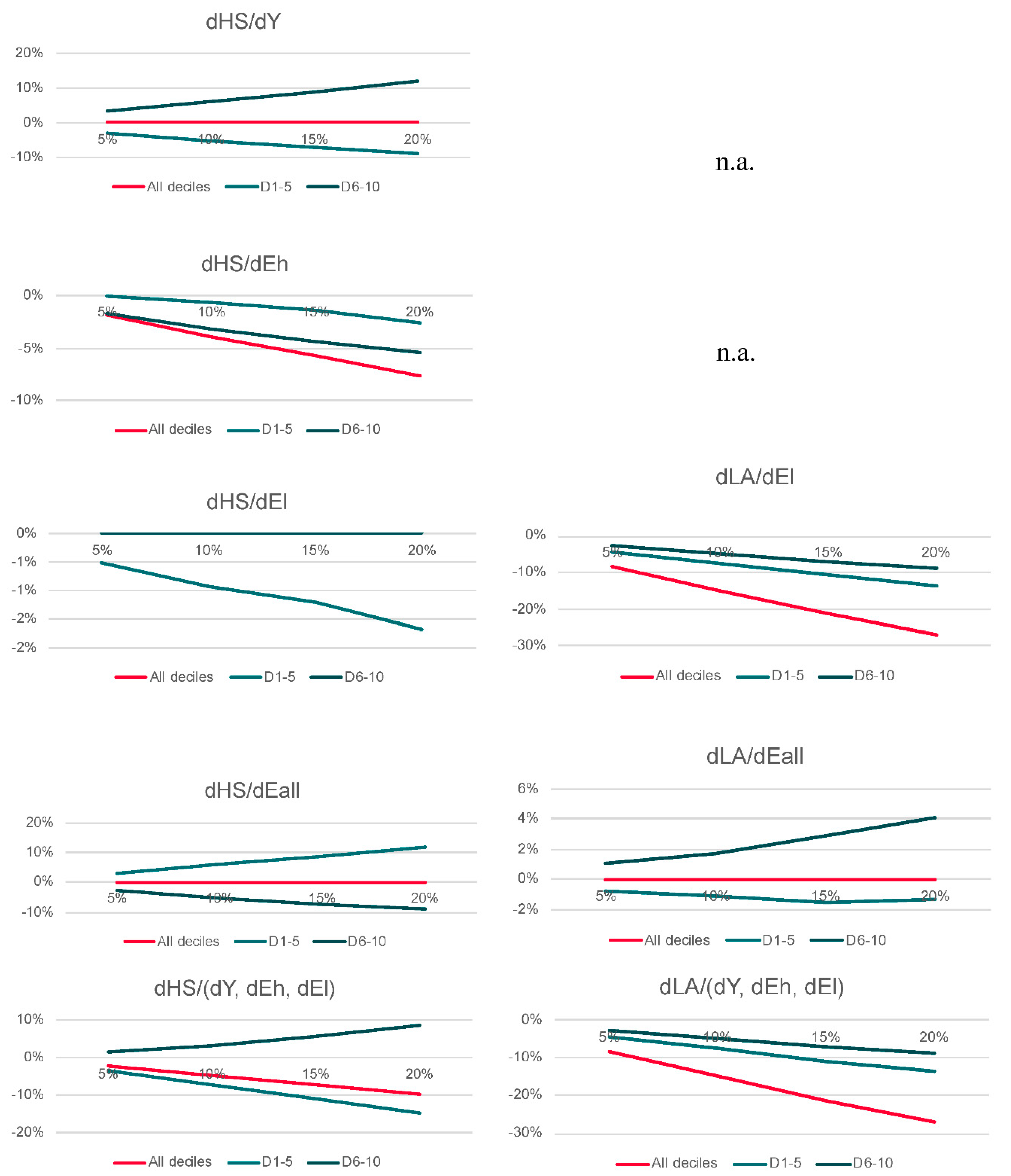
| Differentiation of I | I = HS | I = LA | ||||||
|---|---|---|---|---|---|---|---|---|
| Variation of | Variation | All Deciles | D1-5 | D6-10 | All Deciles | D1-5 | D6-10 | |
| dI/dY | Y↑ | 5% | 0.0% | −2.8% | 3.3% | 0.0% | 0.0% | 0.0% |
| 10% | 0.0% | −5.3% | 6.0% | 0.0% | 0.0% | 0.0% | ||
| 15% | 0.0% | −7.0% | 8.9% | 0.0% | 0.0% | 0.0% | ||
| 20% | 0.0% | −8.8% | 12.0% | 0.0% | 0.0% | 0.0% | ||
| dI/dEh | Eh↓* | 5% | −1.9% | −0.1% | −1.8% | 0.0% | 0.0% | 0.0% |
| 10% | −3.9% | −0.7% | −3.2% | 0.0% | 0.0% | 0.0% | ||
| 15% | −5.8% | −1.5% | −4.4% | 0.0% | 0.0% | 0.0% | ||
| 20% | −7.7% | −2.6% | −5.4% | 0.0% | 0.0% | 0.0% | ||
| dI/dEl | El↑ ** | 5% | −0.5% | −0.5% | 0.0% | −8.3% | −4.2% | −2.5% |
| 10% | −0.9% | −0.9% | 0.0% | −14.8% | −7.4% | −4.8% | ||
| 15% | −1.2% | −1.2% | 0.0% | −21.4% | −10.8% | −7.0% | ||
| 20% | −1.7% | −1.7% | 0.0% | −26.9% | −13.6% | −8.7% | ||
| dI/dEall | Eall↑ | 5% | 0.0% | 3.3% | −2.8% | 0.0% | −0.8% | 1.1% |
| 10% | 0.0% | 6.0% | −5.3% | 0.0% | −1.1% | 1.8% | ||
| 15% | 0.0% | 8.9% | −7.0% | 0.0% | −1.5% | 2.9% | ||
| 20% | 0.0% | 12.0% | −8.8% | 0.0% | −1.3% | 4.1% | ||
| dI/(dY, dEh, dEl) | Y, Eh↓, El↑ | 5% | −2.4% | −3.6% | 1.4% | −8.3% | −4.2% | −2.5% |
| 10% | −4.9% | −7.4% | 3.1% | −14.8% | −7.4% | −4.8% | ||
| 15% | −7.1% | −11.1% | 5.9% | −21.4% | −10.8% | −7.0% | ||
| 20% | −9.8% | −14.7% | 8.6% | −26.9% | −13.6% | −8.7% |
Publisher’s Note: MDPI stays neutral with regard to jurisdictional claims in published maps and institutional affiliations. |
© 2020 by the authors. Licensee MDPI, Basel, Switzerland. This article is an open access article distributed under the terms and conditions of the Creative Commons Attribution (CC BY) license (http://creativecommons.org/licenses/by/4.0/).
Share and Cite
Thema, J.; Vondung, F. Expenditure-Based Indicators of Energy Poverty—An Analysis of Income and Expenditure Elasticities. Energies 2021, 14, 8. https://doi.org/10.3390/en14010008
Thema J, Vondung F. Expenditure-Based Indicators of Energy Poverty—An Analysis of Income and Expenditure Elasticities. Energies. 2021; 14(1):8. https://doi.org/10.3390/en14010008
Chicago/Turabian StyleThema, Johannes, and Florin Vondung. 2021. "Expenditure-Based Indicators of Energy Poverty—An Analysis of Income and Expenditure Elasticities" Energies 14, no. 1: 8. https://doi.org/10.3390/en14010008
APA StyleThema, J., & Vondung, F. (2021). Expenditure-Based Indicators of Energy Poverty—An Analysis of Income and Expenditure Elasticities. Energies, 14(1), 8. https://doi.org/10.3390/en14010008