A Novel Integrated Profit Maximization Model for Retailers under Varied Penetration Levels of Photovoltaic Systems

Abstract

In contemporary energy markets, the Retailer acts as the intermediate between the generation and demand sectors. The scope of the Retailer is to maximize its profits by selecting the appropriate procurement mechanism and selling price to the consumers. The wholesale market operation influences the profits since the mix of generation plants determines the system marginal price (SMP). In the related literature, the SMP is treated as a stochastic variable, and the wholesale market conditions are not taken into account. The present paper presents a novel methodology that aims at connecting the wholesale and retail market operations from a Retailer’s perspective. A wholesale market clearing problem is formulated and solved. The scope is to examine how different photovoltaics (PV) penetration levels in the generation side influences the profits of the Retailer and the selling prices to the consumers. The resulting SMPs are used as inputs in a retailer profit maximization problem. This approach allows the Retailer to minimize economic risks and maximize profits. The results indicate that different PV implementation levels on the generation side highly influences the profits and the selling prices.

1. Introduction

The gradual liberalization and development of a single and competitive energy market has been one of the main pillars of the European Union (EU) energy policy, in the context of the wider changes in the energy sector in past few years [1]. The creation of a liberalized electricity market was considered a key priority by the EU institutions, as it was considered that is an important step towards the completion of the internal energy market, more efficient production, transmission and distribution of electricity, enhancing the security of electricity supply and strengthening the competitiveness of the European economy in conjunction with the protection of the environment [2]. For the last 20 years, the EU has sought a methodical opening of the energy market by distinguishing between competitive, e.g., electricity supply to consumers and non-competitive e.g., grid operation activities, third-party access to their infrastructure, the liberalization of electricity supply activity, the gradual lifting of restrictions on consumer choice of retailer, and the establishment of independent market regulators [3,4,5].

Formerly, the organization of energy companies under the status of legal monopoly, with vertically integrated enterprises, identified the multilateralism of generation, transmission, and distribution activities with the one-sidedness of only one provider of all of these services. With the liberalization of energy markets, an accelerating polymerization manifested into the competing activities of generation and distribution. Commonly, the transition from the monopolizing energy industry in the liberalized energy market is done without the activities of the industry to change numerically, but establishing now the possibility of changes in the number of energy actors in the generation and distribution sectors. The result of these changes was an increase of competitive activities, and the transformation of the state into a regulatory supervisor, who sets the criteria and grants the license to deal with these activities for everyone [6,7].

The Retailer is a new entity in the competitive electricity market. Acting as the intermediate agent between generation and supply, the Retailer has only rights for supplying the demand and not purchase energy through interconnections and bid it in the wholesale market [8]. Within a competitive retail market environment, the scope of the Retailer is to offer competitive energy services to its customers to maximize its profits. The Retailer faces many sources of uncertainties such as the selection of electricity procurement mechanism, market prices, consumers’ behavior, and others. The maximization of profits can be accomplished with the selection of the optimal procurement mechanism, and the definition of the optimal selling price offered to the consumers. The maximization of the profit is an applied mathematical optimization task. Subject to competition, the selling price should lead simultaneously to increased profits and consumers satisfaction [9,10].

There is a variety of studies in the literature that investigate the problem of profit maximization. A Monte Carlo based simulation to extract future loads in order to analyze a set of retailer strategies for balancing settlement risks is used in [11]. The scope is to determine the different levels of demand responses to the profit. The problem of optimal contract design referring to prices and quantities, both at supply and end-user levels is studied in [12]. The proposed methodology allows the Retailer to make robust contractual decisions referred to prices and power quantities. Pool market prices are simulated via an ARIMA model in [13]. Apart from the pool market, the procurement mechanisms include forward contracts (FCs). The model is applied to three types of consumers. A sensitivity analysis of the factors that influence profit takes place in [14]. The parameters are price strategy, i.e., variations between periods, upper price limits, consumer elasticity on prices, and others. An investigation of how the retailer’s decisions related to the risk of pool prices influence the profit is carried out in [15]. The conclusions of the study denote that as the Retailer relies more on the pool market, the profits are increased. This is due to the fact that FC prices are higher than the average pool market price. Pool market prices are derived by a Generalized Autoregressive Conditional Heteroskedasticity (GARCH) model in [16]. The Retailer’s approach towards risk is modeled using the conditional value-at-risk (CVaR) measure. The authors examine how the profit changes taking into account different combinations of procurement mechanisms. In [17], the authors focus on the Chinese electricity market. The Retailer model considers fixed prices and dynamic prices. The procurement mechanisms include bilateral mid-long-term contracts and pool market. The authors conclude that dynamic prices lead to higher profits. However, the difference in profits using fixed and dynamic prices becomes lower when the Retailer increases the amount of purchased electricity from the contracts. In [18], the CVaR measure is employed to balance the amounts between the pool and forward markets. The authors consider the linear price/demand function. For each hour, market prices are calculated as the average of historical prices for that hour, over the entire planning period. In [19], the pricing mechanism is time-of-use (TOU) rates. Market prices are modeled as stochastic variables. The paper introduces the time-series responses of the consumers to the time-varying TOU prices in medium-term planning. In [20], both consumers’ demand and system marginal prices (SMPs) are extracted via a SARIMA model. To reduce the number of scenarios, the K-means clustering algorithm is used. The pool market price series are divided per time period within the day, namely peak, shoulder, and valley periods. The authors conclude that purchasing electricity from various mechanisms results in higher profits than utilizing sole purchase mechanisms. In [21], the focus is placed in the comparison of Value-at-Risk (Var) and CVaR measures considering different FC structures. The CVaR wins the competition and leads to lower profit losses. In [22], the examined electricity market is PJM in the USA. The SARIMA model is utilized to develop 500 scenarios for demand and 500 for price. A discussion is provided on how profit is modified between the scenarios. In [23], market prices and consumers’ demand are assumed known variables and not scenarios-based modeling takes place. No FCs are regarded. The paper considers different Retailers that provide different fixed prices. In [24], the Markowitz theory is regarded to optimize Retailer’s portfolio. The scope is to determine the optimal price per consumer categories, namely, residential, industrial, street lighting, small and large commercial. The results show that the retailer, by being more realistic in choosing consumers to its portfolio, can offer more competitive tariffs to key consumers and keep the portfolio optimal and stable in relation to the risk–return ratio. In [25], the aim is to define the optimal selling price. The Retailer owns a hydrogen storage system containing an electrolyzer, hydrogen storage tanks, and fuel cell. Demand and prices are modeled via a series of scenarios. The power unit, together with the storage, are used as additional mechanisms to cover the demand. In [26], prices and loads are stochastic variables and are extracted through a SARIMA model. The initial 500 scenarios are reduced to 100. Apart from CVaR, the authors examine the application of minimax regret and chance-constrained measures.

It should be mentioned that most of the previous studies consider a fixed selling price. A more accurate pricing mechanism that is able to transfer the costs of generated electricity to the end consumers is real-time pricing (RTP) [27]. RTP is a concept that belongs to the family of price-based demand response (DR) methods. Contrary to an incentive-based DR, the consumers participation and response in a price-based DR is not mandatory [28]. The RTP scheme is examined considering various price/demand functions in [29]. The authors examine the influence of the selection of different functions in the profits. Load profiling information is used in [30,31]. The general approach of these studies is: A clustering is applied to a group of consumers, and clusters of consumers with similar characteristics are formed. The profit maximization problem per cluster is solved, and the selling price per consumer clusters is defined.

Based on the previous literature overview, the main conclusions that can be drawn are:

(i)

All the studies concerned with the Retailer profit maximization problem do not involve wholesale market clearing problems. The wholesale operation is not examined, and thus potential changes in the electricity generation mix are not validated in terms of retail market conditions. More specifically, there is little evidence in the literature on how increased capacity of renewably energy influences the cost of electricity and the RTP offered to the consumers that reflect this cost.

(ii)

The pool market prices are simulated as stochastic variables through a scenarios based approach. By incorporating stochastic programming simulations in mixed-integer linear problems, the overall complexity of the optimization problem increases.

(iii)

The topic of dynamic pricing has not received considerable attention. In the majority of the studies the selling price is fixed and not time-variant.

In the present study, the focus is to replace the stochastic programming approach by providing a market-clearing solution on the wholesale side. An integrated profit maximization model is proposed. The term integration refers to the connection between wholesale and retail markets. The proposed model includes a wholesale side and a retail side models. A market-clearing problem is solved to extract the SMP for various photovoltaics (PV) implementation scenarios. More specifically, the market-clearing problem is solved hourly for a full year. The scope of the scenarios is to assess how the implementation of different renewable generation capacity of an energy system influences the Retailer actions and the selling price limits. Based on the DR model that simulates the consumers’ behavior on the price, the final selling price is derived and sent to the consumers. It is assumed that the consumers react rationally and modify their load accordingly. Then, the profitability, i.e., the ratio of revenue to income is calculated. The proposed model is flexible; different wholesale market conditions can be simulated in detail; different procurement mechanisms can be exploited together with various types of dynamic pricing.

2. Methodology

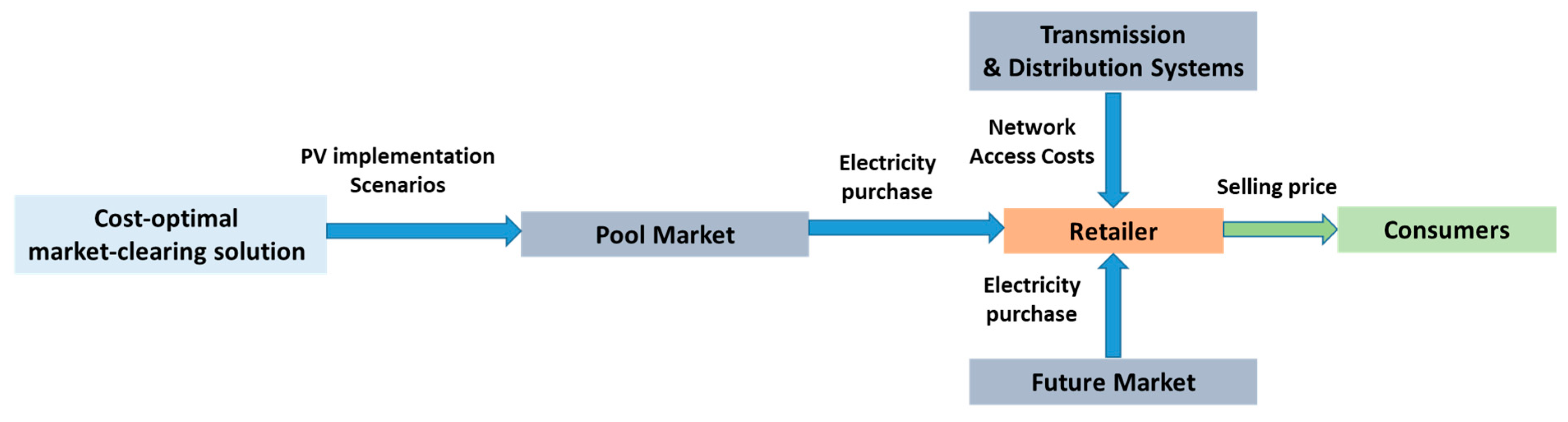
2.1. General Framework

The schematic representation of the proposed model is shown in Figure 1. Apart from the generation mix, interconnections interchanges, and others, the outputs of the cost-optimal market-clearing problem include the hourly SMPs for a full year. The number of SMP time series equals the number of PV implementation scenarios. Two procurement mechanisms are regarded, namely the future market and pool market. The outputs of the profit maximization problem include the RTPs transferred to the consumers.

2.2. Mathematical Formulation of the Wholesale Market Optimization Model

This part deals with the cost-optimal market-clearing of a power system, considering the power units’ operational constraints and interconnections with neighboring power systems. The examined period is a daily one, with an hourly time step $t$. The power units taken into consideration include thermal power ones $th$, nuclear $nu$, hydroelectric $h$, and renewable energy ones $r$. Thermal power units, along with nuclear power ones, are commonly referred to as type-$l$ units. Additional sources of supply are the electricity imports $m$ from neighboring power systems, while electricity exports $x$ can also be carried to the same systems. Both supply and consumption entities offer/bid specific quantities at certain prices. Each offer/bid is also divided into a number of blocks with a non-decreasing (increasing) order for offers (bids). In particular:

• price ($C_{l,bl,t}^{unit}$)—quantity ($C{B}_{l,bl,t}$) pair for the energy supply of type-$l$ power units,
• price ($C_{m,bl,t}^{imp}$)—quantity ($C{B}_{m,bl,t}$) pair for the energy supply of electricity imports $m$,
• price ($C_{x,bl,t}^{exp}$)—quantity ($C{B}_{x,bl,t}$) pair for the energy consumption of electricity exports $x$, and
• price ($C_{d,bl,t}^{dm}$)—quantity ($C{B}_{d,bl,t}$) pair for the energy consumption of electricity demand bids $d$.

A specific cost ($C_{h,t}^{hr}$) is assigned with the cleared electricity supply from hydroelectric units, which is dependent on the assumed hydrological conditions of the specific date $dt$ ($E_{dt}^{hyd}$), and the hourly availability of each hydroelectric unit $h$ ($P_{h,t}^{max}$). Concerning the renewable energy units $r$, a certain cost ($C_{r,t}^{hr}$) is associated with the cleared electricity supply from renewable energy units, based on the assumed meteorological conditions for each type of resource $r$ and time period $t$ ($A{V}_{r,t}$), and the installed capacity of each renewable energy source $r$ ($P_r^{max}$).

Each energy supply unit $l$ is characterized by a specific technical maximum ($P_l^{max}$) and minimum ($P_l^{min}$) for their operation. Specific limits exist in their ability to increase (up) or decrease (down) their outputs, commonly referred to as ramp-up ($R{U}_l$) and ramp-down limits ($R{D}_l$). Moreover, type-$l$ units are identified based on their minimum uptimes ($T_l^{UT}$) and downtimes ($T_l^{DT}$).

When they provide secondary reserve, they should operate under Automatic Generation Control (AGC), in which they have other technical maximums ($P_l^{max,AGC}$) and minimums ($P_l^{min,AGC}$). Type-$l$ units can also provide reserves to the systems that can be primary-up and -down, secondary-up and –down, and tertiary upward spinning and non-spinning. This reserve supply has a specific cost based on the type of reserve, the type of supplier $l$, and the time period $t$, namely, $C_{l,t}^{1up}$, $C_{l,t}^{1dn}$, $C_{l,t}^{2up}$, $C_{l,t}^{2dn}$, and $C_{l,t}^3$ for primary-up, primary–down, secondary-up, secondary-down, and tertiary reserve. Further, there are upper bounds for the provision of each type of reserve per unit $l$, namely, $R_l^{1up}$ for primary-up, $R_l^{1dn}$ for primary-down, $R_l^{3s}$ for tertiary spinning, and $R_l^{3ns}$ for tertiary non-spinning reserve. The maximum level for the provision of the secondary-up and –down reserve is related to the ramp-up ($R{U}_l^{AGC}$) and down limits ($R{U}_l^{AGC}$) of each unit l when operating under AGC. Two other cost components are associated with the start-up ($C_l^{stu}$) and the shut-down ($C_l^{shd}$) decision making of each type-$l$ unit. Furthermore, the cases of unmet energy ($C_t^{ue}$) or inability to cover part of reserve requirements per type have been assigned with specific cost penalties ($C_t^{ur}$).

The system’s requirements for each reserve type include:

• primary-up reserve requirements ($D{R}_t^{1up}$),
• primary-down reserve requirements ($D{R}_t^{1dn}$),
• secondary-up reserve requirements ($D{R}_t^{2up}$),
• secondary-down reserve requirements ($D{R}_t^{2dn}$), and
• tertiary reserve requirements ($D{R}_t^3$).

2.2.1. Objective Function of the Wholesale Market Optimization Problem

The mathematical model’s objective function refers to minimizing a given power system’s daily energy and reserves cost as provided by the following relationship (1).

$$\begin{array}{c}Min C^{total}=\\ {\displaystyle \stackrel{Thermal-Nuclear}{\overbrace{{\displaystyle \sum }_l{\displaystyle \sum }_{bl}{\displaystyle \sum }_t{C}_{l,bl,t}^{unit}·b_{l,bl,t}}}+\stackrel{Hydro-RES}{\overbrace{{\displaystyle \sum }_{hr}{\displaystyle \sum }_t{C}_{hr,t}^{hr}·p_{hr,t}}}+\stackrel{Imports}{\overbrace{{\displaystyle \sum }_m{\displaystyle \sum }_{bl}{\displaystyle \sum }_t{C}_{m,bl,t}^{imp}·b_{m,bl,t}}}}\\ {\displaystyle \stackrel{Start-up cost}{\overbrace{+{\displaystyle \sum }_l{\displaystyle \sum }_t{C}_l^{stu}·y_{l,t}}}+\stackrel{Shut-down cost}{\overbrace{{\displaystyle \sum }_l{\displaystyle \sum }_t{C}_l^{shd}·z_{l,t}}}+\stackrel{Energy unmet cost}{\overbrace{{\displaystyle \sum }_{t}n{d}_t·C_t^{ue}}}}\\ {\displaystyle -\stackrel{Exports revenues}{\overbrace{{\displaystyle \sum }_x{\displaystyle \sum }_{bl}{\displaystyle \sum }_t{C}_{x,bl,t}^{exp}·b_{x,bl,t}}}-\stackrel{Demand revenues}{\overbrace{{\displaystyle \sum }_d{\displaystyle \sum }_{bl}{\displaystyle \sum }_t{C}_{d,bl,t}^{dm}·b_{d,bl,t}}}}\\ {\displaystyle \stackrel{Primary-up cost}{\overbrace{+{\displaystyle \sum }_l{\displaystyle \sum }_t{C}_{l,t}^{1up}·r_{l,t}^{1up}}}\stackrel{Primary-down cost}{\overbrace{+{\displaystyle \sum }_l{\displaystyle \sum }_t{C}_{l,t}^{1dn}·r_{l,t}^{1dn}}}+\stackrel{Secondary-up cost}{\overbrace{{\displaystyle \sum }_l{\displaystyle \sum }_t{C}_{l,t}^{2up}·r_{l,t}^{2up}}}+\stackrel{Secondary-down cost}{\overbrace{{\displaystyle \sum }_l{\displaystyle \sum }_t{C}_{l,t}^{2dn}·r_{l,t}^{2dn}}}}\\ {\displaystyle +\stackrel{Tertiary cost}{\overbrace{{\displaystyle \sum }_l{\displaystyle \sum }_t{C}_{l,t}^3·r_{l,t}^3}}+\stackrel{Reserves unmet cost}{\overbrace{{\displaystyle \sum }_t{C}_t^{ur}·\left(n{v}_t^{1up}+n{v}_t^{1dn}+n{v}_t^{2up}+n{v}_t^{2dn}+n{v}_t^3\right)}}}\end{array}$$

(1)

2.2.2. Energy Demand Balance

This section provides the mathematical set-up of the energy demand balance.

$${\displaystyle \sum }_{th}{p}_{th,t}+{\displaystyle \sum }_{nu}{p}_{nu,t}{\displaystyle \sum }_h{p}_{h,t}+{\displaystyle \sum }_r{p}_{r,t}+{\displaystyle \sum }_m{p}_{m,t}+n{d}_t={\displaystyle \sum }_d{p}_{d,t}+{\displaystyle \sum }_x{p}_{x,t} \forall t$$

(2)

Equation (2) states that the total energy supply from all types of suppliers, including thermal $th$, nuclear $nu$, hydroelectric $h$, renewable energy units $r$ and imports $m$ plus the amount of unmet demand must meet the cleared demand bids $d$ and energy exports $x$ in each time period $t$.

2.2.3. Operational Constraints

This set of constraints refers to operational limits. The available capacity of each energy supply entity $l$, $m$, and consumption entity x and d is divided into a number of blocks $bl$, each of which has a unique price-quantity pair.

$$b_{l,bl,t}\le C{B}_{l,bl,t} \forall l,bl,t$$

(3)

$$b_{m,bl,t}\le C{B}_{m,bl,t} \forall m,bl,t$$

(4)

$$b_{x,bl,t}\le C{B}_{x,bl,t }\forall x,bl,t$$

(5)

$$b_{d,bl,t}\le C{B}_{d,bl,t} \forall d,bl,t$$

(6)

$$p_{l,t}={\displaystyle \sum }_{bl}{b}_{l,bl,t} \forall l,t$$

(7)

$$p_{m,t}={\displaystyle \sum }_{bl}{b}_{m,bl,t} \forall m,t$$

(8)

$$p_{x,t}={\displaystyle \sum }_{bl}{b}_{x,bl,t} \forall x,t$$

(9)

$$p_{d,t}={\displaystyle \sum }_{bl}{b}_{d,bl,t} \forall d,t$$

(10)

$$p_{l,t}+r_{l,t}^{2up}\le P_l^{max}·\left(x_{l,t}-x_{l,t}^{AGC}\right)+P_l^{max,AGC}·x_{l,t}^{AGC}\forall l,t$$

(11)

$$p_{l,t}-r_{l,t}^{2dn}\ge P_l^{min}·\left(x_{l,t}-x_{l,t}^{AGC}\right)+P_l^{min,AGC}·x_{l,t}^{AGC} \forall l,t$$

(12)

$$p_{l,t}+r_{l,t}^{1up}+r_{l,t}^{2up}+r_{l,t}^{3s}\le P_l^{max}·x_{l,t} \forall l,t$$

(13)

$$p_{l,t}-r_{l,t}^{1dn}-r_{l,t}^{2dn}\ge P_l^{min}·x_{l,t} \forall l,t$$

(14)

The cleared energy supply of each supply entity $l$ ($m$) in each block $bl$ and time period $t$ has the upper limit of the corresponding offered quantity, according to constraints (3) and (4). Constraints (5) and (6) defines that the cleared energy exports to each interconnected power system $x$ (demand bids $d$) in each block $bl$ and time period $t$ must not exceed the corresponding available quantity. Equations (7) and (8) set that the total cleared energy supply from each entity $l$ ($m$) in each time period $t$ amounts to the sum of all blocks of the respective cleared energy supply. The total cleared electricity exports to each interconnected power system $x$ (demand bids d) in each interval $t$ amount to the sum of all blocks of the corresponding cleared energy exports (demand bids), according to Equations (9) and (10). Constraints (11)–(14) model the operational limits, upper ((11) and (13)) and lower ((12) and (14)) respectively, of each unit $l$ in each interval $t$, also considering their reserve provision capabilities (primary-up, primary-down, secondary-up and –down, and tertiary spinning).

2.2.4. Reserve Provision Limits

This section provides the mathematical set-up of the reserve provision limits.

$$r_{l,t}^{1up}\le R_l^{1up}·x_{l,t} \forall l,t$$

(15)

$$r_{l,t}^{1dn}\le R_l^{1dn}·x_{l,t} \forall l,t$$

(16)

$$r_{l,t}^{2up}\le 15·R{U}_l^{AGC}·x_{l,t}^{AGC} \forall l,t$$

(17)

$$r_{l,t}^{2dn}\le 15·R{D}_l^{AGC}·x_{l,t}^{AGC} \forall l,t$$

(18)

$$r_{l,t}^{3s}\le R_l^{3s}·x_{l,t} \forall l,t$$

(19)

$$r_{l,t}^{3ns}\le R_l^{3ns}·x_{l,t}^{3ns} \forall l,t$$

(20)

$$r_{l,t}^{3ns}\ge P_l^{min}·x_{l,t}^{3ns} \forall l,t$$

(21)

$$r_{l,t}^{3ns}\le R_l^{3ns}·\left(1-x_{l,t}\right) \forall l,t$$

(22)

$$p_{l,t}-p_{l,t-1}\le R{U}_l·60 \forall l,t$$

(23)

$$p_{l,t-1}-p_{l,t}\le R{D}_l·60 \forall l,t$$

(24)

This set of constraints (15)–(22) models the reserve provision limits of each reserve supplier $l$ in each time period $t$, by imposing upper limits for each reserve type, subject to the entity’s dispatch ($x_{l,t}$) or not ($1-x_{l,t}$), and operation under AGC or not ($x_{l,t}^{AGC}$). More specifically, constraint (15) puts an upper bound on the primary-up reserve supply, constraint (16) on the primary-down reserve supply, constraint (17) on the secondary-up reserve supply, constraint (18) on the secondary-down reserve supply, constraint (19) on the tertiary-spinning reserve supply, and constraints (20)–(22) on the tertiary non-spinning reserve supply. Constraints (23) and (24) define the ramp-up ($R{U}_l$) and -down ($R{D}_l$) limits, for each entity $l$ in each interval $t$, namely the rate at which a supplying entity can increase (up) or decrease (down) its output.

2.2.5. System’s Reserve Requirements

This section provides the mathematical set-up of the system’s reserve requirements.

$${\displaystyle \sum }_{ht}{r}_{ht,t}^{1up}+n{v}_t^{1up}\ge D{R}_t^{1up} \forall t$$

(25)

$${\displaystyle \sum }_{ht}{r}_{ht,t}^{1dn}+n{v}_t^{1dn}\ge D{R}_t^{1dn} \forall t$$

(26)

$${\displaystyle \sum }_{ht}{r}_{ht,t}^{2up}+n{v}_t^{2up}\ge D{R}_t^{2up} \forall t$$

(27)

$${\displaystyle \sum }_{ht}{r}_{ht,t}^{2dn}+n{v}_t^{2dn}\ge D{R}_t^{2dn} \forall t$$

(28)

$${\displaystyle \sum }_{ht}\left(r_{ht,t}^{3s}+r_{ht,t}^{3ns}\right)+n{v}_t^3=r_{ht,t}^3\ge D{R}_t^3 \forall t$$

(29)

The following group of constraints (25)–(29) defines the system-wide requirements for each reserve type, primary-up (25), primary-down (26), secondary-up (27), secondary-down (28), and tertiary spinning and non-spinning (29), respectively, which can be provided by hydrothermal units $ht$, namely hydroelectric and thermal power units plus the amount of unmet demand per reserve type.

2.2.6. Renewable Energy Generation

This section provides the mathematical set-up of renewable energy generation.

$$p_{r,t}+n{r}_{r,t}\le A{V}_{r,t}·P_r^{max } \forall r,t$$

(30)

Equation (30) imposes that the energy supply of each renewable energy technology $r$ in each interval $t$ ($p_{r,t}$) plus the amount of the corresponding curtailed energy ($n{r}_{r,t}$) has an upper bound related to the availability of each renewable energy technology $r$ in each interval $t$ ($A{V}_{r,t}$) multiplied with its installed capacity in each interval $t$ ($C{C}_{r,t}$).

2.2.7. Hydroelectric Power Generation

This section provides the mathematical set-up of hydroelectric power generation.

$${\displaystyle \sum }_h{\displaystyle \sum }_{t\in dt}{p}_{h,t}\le E_{dt}^{hyd} \forall dt$$

(31)

$$p_{h,t}\le P_{h,t}^{max} \forall h,t$$

(32)

Constraint (31) imposes that the daily energy supply from all hydropower units $h$ in each date $dt$ of the year (${\displaystyle \sum }_h{\displaystyle \sum }_{t\in dt}{p}_{h,t}$) must not exceed a specific maximum bound ($E_{dt}^{hyd}$). In addition, Constraint (32) states that the daily maximum must not exceed the total available installed capacity.

2.2.8. Time-Related Constraints

This section provides the mathematical set-up of the time-related constraints.

$${\displaystyle \sum }_{t^{\prime }=t-T_l^{UT}+1}^t{y}_{l,t^{\prime }}\le x_{l,t} \forall l,t$$

(33)

$${\displaystyle \sum }_{t^{\prime }=t-T_l^{DT}+1}^t{z}_{l,t^{\prime }}\le 1-x_{l,t} \forall l,t$$

(34)

$$y_{l,t}-z_{l,t}=x_{l,t}-x_{l,t-1} \forall l,t$$

(35)

$$x_{l,t}^{AGC}\le x_{l,t} \forall l,t$$

(36)

Constraint (33) models the minimum uptime of each supply unit $l$, based on which it must be online in each interval $t$ ($x_{l,t}=1$) if and only if it has started-up ($y_{l,t}=1$) during the previous ($T_l^{UT}-1$) intervals. Analogously, Constraint (34) defines the minimum downtime of each supply unit $l$, according to which it must remain offline in each interval $t$ ($x_{l,t}=0$) if it has been down ($z_{l,t}=1$) during the previous ($T_l^{DT}-1$) intervals. Moreover, Equation (35) formulates the logical relationship between start-up ($y_{l,t}$) and shut-down ($z_{l,t}$) decisions of each supply entity $l$ in each time period $t$. Furthermore, a supply entity l can operate under AGC if and only if it operates in the dispatch phase, according to Constraint (36).

2.2.9. Net Electricity Trading

This section provides the mathematical set-up of the net electricity trading.

$$p_{m,t}-p_{x,t} \le {\displaystyle \sum }_{bl}{b}_{m,bl,t} \forall \left(m,x\right) \in MX,t$$

(37)

$$p_{x,t}-p_{m,t}\le {\displaystyle \sum }_{bl}{b}_{x,bl,t} \forall \left(m,x\right) \in MX,t$$

(38)

Constraint (37) states that net electricity imports ($p_{m,t}-p_{x,t}$) of each interconnection (imports) $m$ in each time period$t$, also considering their reserve supply capability, must not exceed the corresponding interconnection capacity (${\displaystyle \sum }_{bl}{b}_{m,bl,t}$). Further, Constraint (38) sets the same condition for net electricity exports ($p_{x,t}-p_{m,t}$).

The overall problem is formulated as a mixed-integer linear programming (MILP) problem, involving the cost minimization objective function (1), and subject to Constraints and Equations (2)–(38).

2.3. Mathematical Formulation of the Retail Market Optimization Model

The decision making actions of the Retailer are classified into medium-term and short-term actions. The medium-term actions determine the electricity purchased from the future market via forwards contracts (FCs). After this decision, the short-term actions define the amount purchased from the pool market and the selling price. Below the formulation of the retail market optimization model is analyzed.

2.3.1. Future Market

In order to form the FCs structure, it is necessary to categorize the 24 h period into various intra-day periods, according to the following:

• Period#1={01:00,02:00,03:00,04:00,05:00,06:00,07:00,08:00,09:00,10:00,11:00,12:00,13:00,14:00}
• Period#2={15:00,16:00,17:00,18:00}
• Period#3={19:00, 20:00,21:00, 22:00}
• Period#4={23:00,24:00}

Period#3 refers to peak hours while the remaining to off-peak hours. Based on these periods five FCs are considered, which differ intra-day wise. Each FC is composed of five blocks that correspond to each power amount that differ in the price. The block limits are 20, 40, 60, 80, and 100 kW. Let $f=1,2,\dots ,F$ be the number of FCs and $j=1,2,\dots ,N_j$ the number of blocks. The cost $C_t^F$ that is related to the FCs in period $t$is calculated by

$$C_t^F={\displaystyle \sum _{f\in F}{\displaystyle \sum _{j=1}^{N_j}{\lambda }_{fjt}^F}{P}_{fjt}^F,\forall t}$$

(39)

$$0\le P_{fjt}^F\le P_{fjt,\max }^F,\forall f,j,t$$

(40)

$$P_{ft}^F={\displaystyle \sum _{j=1}^{N_j}{P}_{ftj}^F},\forall f,t$$

(41)

where ${\lambda }_{fjt}^F$ and $P_{fjt}^F$ are the price and amount purchased from $f$-th contract and $N_j$-th block, respectively, at period $t=1,2,\mathrm{..},T$. Parameter $P_{fjt,\max }^F$ denotes the block size. Equation (40) sets a limit of the amount to be purchased of each block. The term refers to the maximum power offered by the specific FC, i.e., it refers to the block size. Equation (41) refers to the total power of each contract $P_{fjt}^F$ which is given as the sum of the powers of each block.

2.3.2. Pool Market

After the solution of the market-clearing problem, the SMPs are available. Let ${\lambda }_t^P$ be the price in the pool market at period $t=1,2,\mathrm{..},T$. The cost of energy purchased from the pool $C_t^P$ is expressed as

$$C_t^P={\lambda }_t^P\cdot E_t^P,\forall t$$

(42)

where $E_t^P$ is the energy purchased for the pool at period $t$.

2.3.3. Demand Response

It is considered that the Retailer serves one group of consumers of the same type. The responsiveness of the consumers to the selling price is modeled through a linear price/demand function. This means that when consumers are offered a high selling price, they linearly decrease their demand.

Initially, the consumers are charged with a nominal selling price $r_o$ at period $t=1,2,\mathrm{..},T$. After the solution of the retail optimization problem, a new price is offered that maximizes Retailer’s profit. Let $r(t)$ be a random selling price at period $t=1,2,\mathrm{..},T$ after the solution of the problem. Due to the nominal price $r_o$ the consumers’ nominal demand is indicated as $d_o.$ The demand response of the consumers to the selling price $r(t)$ is denoted as $d(t).$The linear price/demand function is expressed as

$$d(r(t))=d_o\left\{1+\frac{\beta [r(t)-r_o]}{r_o}\right\}$$

(43)

The parameter that controls the level of the demand variation is the elasticity $\beta .$

2.3.4. Demand Balance

To reach out into a feasible solution to the problem, an energy balance constraint should be imposed. For each time instant $t$ the demand of the consumers $E_t^D$ should be covered by two procurement mechanisms:

$$E_t^D=E_t^P+{\displaystyle \sum _{f\in F}{P}_{ft}^F},\forall t$$

(44)

To correspond to formulation of the problem, Equation (43) is rewritten as

$$E_t^D=E_{ot}^D\left\{1+\frac{\beta \left({\lambda }_t^D-{\lambda }_{ot}^D\right)}{{\lambda }_{ot}^D}\right\},\forall t$$

(45)

where $E_{ot}^D$ is the nominal demand, ${\lambda }_{ot}^D$ is the nominal selling price and ${\lambda }_t^D$ is the selling price at period $t=1,2,\mathrm{..},T$.

2.3.5. Selling Price Limit

Theoretically, the higher the offered price the higher the profits will be. In order for the Retailer to become competitive and follow the rules of the market set by the regulatory authorities, a price limitation is needed. If the consumers elasticity would be extremely low, the selling price would correspond to unrealistic high values without price limitation. The price limitation is given by the following equation:

$${\displaystyle \sum _{t=1}^{{\rm T}}{E}_t^D{\lambda }_t^D\le {\lambda }_{\max }^D{\displaystyle \sum _{\tau =1}^{{\rm T}}{E}_t^D}}$$

(46)

where ${\lambda }_{\max }^D$ is the upper limit of the selling price.

2.3.6. Expected Profit and Network Access Costs

The expected profit is obtained by the difference between the revenues and the costs. The revenues $R_t$ refer to the product between the selling price and the consumers’ load:

$$R_t={\lambda }_t^D{E}_t^D,\forall t$$

(47)

Apart from the costs related with the electricity procurement, the retailer is charged with transmission and distribution system access tariffs $C^N$:

$$C^N={\displaystyle \sum _t\left({\lambda }_{et}{E}_t^D+{\lambda }_{pt}{P}_t\right)}$$

(48)

where ${\lambda }_{et}$ and ${\lambda }_{pt}$ are the energy and power elements of the network access tariff, respectively and $P_t$ Is the contracted power.

The Retailer’s profit $RP$ is expressed as

$$RP={\displaystyle \sum _t\left(R_t-C_t^P\right)-{\displaystyle \sum _t{C}_t^F}-C^N=}{\displaystyle \sum _t\left[\left({\lambda }_t^D{E}_t^D-{\lambda }_t^P{{\rm E}}_t^P-{\lambda }_{et}{E}_t^D-{\lambda }_{pt}{P}_t\right)-{\displaystyle \sum _{f\in F}{\displaystyle \sum _{j=1}^{N_j}{\lambda }_{fjt}^F}{P}_{fjt}^F}\right]}$$

(49)

The profit function is composed of elements that refer to incomes and expenses.

2.3.7. Objective Function of the Retail Market Optimization Problem

The profit maximization problem is formulated as

$$\begin{array}{l}{\mathrm{Maximize}}_{P_{fjt}^F,{\lambda }_t^D,E_t^P}\\ {\displaystyle \sum _{t=1}^{N_T}\left[\left({\lambda }_t^D{E}_t^D-{\lambda }_t^P{{\rm E}}_t^P-{\lambda }_{et}{E}_t^D-{\lambda }_{pt}{P}_t\right)-{\displaystyle \sum _{f\in F}{\displaystyle \sum _{j=1}^{N_j}{\lambda }_{fjt}^F}{P}_{fjt}^F}\right]}\end{array}$$

(50)

Subject to: (40), (44) and (46).

3. Results

Both the cost-optimal market-clearing and profit maximization problems are formulated as mixed-integer nonlinear problems and are solved by commercial software [32]. The proposed methodological framework for the wholesale market clearing problem has been assessed on an illustrative case study, the key characteristics of which are provided in

Table 1. Main economic data of the studied power system.

Unit	Start-Up Cost (€/Start-Up)	Shut-Down Cost (€/Shut-Down)	CO2 Emission Factor (tnCO2/MWh)	CO2 Price (€/tnCO2)	Fuel Price (€/t for Lignite and €/MWhth for Natural Gas)	Fuel Heating Value (GJ/t for Lignite)	Efficiency (p.u.)	O&M Cost (€/MWh)	Minimum Average Variable Cost (€/MWh)
LIG-1	50,000	20,000	1.5	25	19.56	4.88	0.38	2.65	78.50
LIG-2	50,000	20,000	1.4	25	7.50	4.29	0.33	1.50	55.46
LIG-3	50,000	10,000	1.3	25	21.00	7.33	0.38	2.14	62.10
LIG-4	50,000	10,000	1.2	25	15.77	4.77	0.33	1.85	67.43
NGCC-1	20,000	10,000	0.37	25	15.35	0.00	0.58	1.20	37.04
NGCC-2	20,000	10,000	0.37	25	15.35	0.00	0.57	1.20	37.58
NGCC-3	20,000	10,000	0.37	25	15.35	0.00	0.58	1.20	37.08
NGCC-4	20,000	10,000	0.37	25	15.35	0.00	0.60	1.20	36.03
NGCC-5	20,000	10,000	0.37	25	15.35	0.00	0.58	1.20	36.99
NGCC-6	20,000	10,000	0.37	25	15.35	0.00	0.51	1.20	40.76
NGGT-1	2500	1000	0.53	25	30.00	0.00	0.40	1.20	89.45
NGGT-2	2500	1000	0.53	25	30.00	0.00	0.40	1.20	89.45
HYDRO	0	0	0	25	0.00	0.00	0.00	0.00	3.00

and

Table 2. Main technical data of the studied power system.

Unit	Technical Maximum (MW)	Technical Minimum (MW)	Technical Maximum under AGC (MW)	Technical Minimum under AGC (MW)	Primary-Up Reserve Capability (MW)	Ramp-Up Limit under AGC (MW/min)	Ramp-Down Limit under AGC (MW/min)	Tertiary Spinning Reserve Capability (MW)	Tertiary Non-Spinning Reserve Capability (MW)	Ramp-Up Limit (MW/min)	Ramp-Down Limit (MW/min)	Minimum Uptime (h)	Minimum Downtime (h)
LIG-1	342	188	0	0	28	0	0	45	0	4	4	16	1
LIG-2	289	151	0	0	28	0	0	45	0	4	4	16	1
LIG-3	256	195	0	0	28	0	0	45	0	4	4	16	1
LIG-4	273	150	0	0	28	0	0	45	0	4	4	16	1
NGCC-1	378	220	360	240	36	12	12	340	340	12	12	12	3
NGCC-2	422	195	390	220	36	12	12	380	380	12	12	12	3
NGCC-3	390	220	370	240	36	10.5	10.5	351	351	10.5	10.5	12	3
NGCC-4	433	195	390	220	36	14	14	390	390	14	14	12	3
NGCC-5	417	182	390	200	36	19.2	19.2	375	375	24	24	12	3
NGCC-6	550	94	550	94	36	12	12	495	495	12	12	12	3
NGGT-1	150	50	120	63	8	7	7	120	120	8	8	1	1
NGGT-2	160	55	128	69	8	7	7	125	125	8	8	1	1
HYDRO	1000	0	1000	25	0	150	150	1000	1000	150	150	0	0

. Table 1 summarizes the studied power system’s economic data, and Table 2, the key technical data. The examined power system includes four LIGnite-fired units (LIG), six Natural Gas Combined Cycle (NGCC) units, two Natural Gas-fired Gas Turbines (NGGT), and hydroelectric units. It additionally includes wind turbines and solar panels, each of which with a capacity of 1 GW. The available interconnection capacity for both imports and exports is assumed to be 2 GW.

The Hellenic energy system serves as the test system where both models are applied [33]. A general test case with a Retailer covering the demand of 84 residential consumers is regarded. The load series refer to the aggregated load of the consumers, and the network access tariffs correspond to the ones of the Hellenic system. The nominal electricity selling tariff $r_o$ is obtained by the sum of the SMP, transmission, and distribution network access tariffs increased by 10%. Following this approach, the Retailer charges the consumers an amount of 10% higher than the nominal, i.e., initial costs related to the pool market. This amount is considered in order to cover some of the operational expenses of the Retailer. The elasticity parameter is $\beta =-\mathrm{1.50.}$ Hence, it is considered that all consumers are very elastic in modifying the demand for small price changes. For simplicity reasons, it is considered that the elasticity is the same for all hours of the day and that all consumers are characterized by the same elasticity. It is assumed that the Retailer is a limited portfolio, i.e., its decisions in the retailer market do not influence retail and wholesale markets operation and conditions.

To fully examine the influence of various implementation rates of PV capacity in the wholesale market, eight scenarios are regarded, denoted as $S_s,s=1,2,\mathrm{\dots },8$.

Table 3. Solutions of the market-clearing problem.

Scenario	S1	S2	S3	S4	S5	S6	S7	S8
PV (MW)	1000	2000	3000	4000	5000	6000	7000	8564
Lignite (GWh)	1042.02	975.23	764.25	521.05	391.56	302.43	341.85	1751.242
Natural gas (GWh)	13,944.41	14,163.34	13,923.14	13,583.90	13,425.54	13,060.16	13,537.81	12,970.15
Hydro (GWh)	1026.92	1026.92	1026.92	1026.92	1026.92	1026.92	1026.92	1026.92
RES (GWh)	3748.20	5183.42	6614.80	7981.51	8907.63	9427.45	9294.21	9029.44
Imports (GWh)	1523.43	983.0232	811.01	525.06	314.15	294.04	180.33	141.94
Exports (GWh)	−5652.59	−6699.54	−7507.73	−8006.06	−8433.40	−8478.60	−8748.74	−9287.30
Demand (GWh)	15,632.41	15,632.41	15,632.41	15,632.41	15,632.41	15,632.41	15,632.41	15,632.41
RES curtailment (GWh)	0	0	3.84	72.35	581.45	1496.85	3065.31	5576.03
Unmet energy (GWh)	0	0	0	0	0	0	0	0
Marginal Price (€/MWh)	49.17	48.40	46.84	44.02	40.17	37.64	35.44	33.14

shows the solutions of the market-clearing problem for a full year. It is shown the amount of annual PV installed capacity. Scenario S1 refers to 1000 MW while S8 to 8564 MW. Due to these different PV capacity mixes, there are visible variations in the capacities of the other technologies and the imports/exports balance. As the PVs shares in the electricity mix increases, thermal units are displaced. More specifically, there is a decrease in the generation of lignite and NG fueled units. Moreover, for 3000 MW generation and higher RES curtailments appear. RES technologies, apart from PVs, include onshore wind turbines and small hydroelectric plants. The last row of the Table presents the annual average SMP. It can be noticed that from S1 to S8, the mean SMP is decreased by 32.60%, i.e., from 49.17 €/MWh to 33.14 €/MWh. While expensive technologies are displaced, the cost of electricity decreases. It is assumed that the PV generation is compensated by a feed-in-tariff mechanism, i.e., all the generated amount is fed into the grid covering a specific part of the demand. The variations of the daily average SMPs time series are depicted in Figure 2. The figure presents the mean annual SMP per scenario.

To thoroughly investigate the influence of the various PV generation shares on the Retailer’s profits and the levels of electricity rates to the end-consumers, four cases are taken into account. The retail market optimization problem is solved for four different days in the year, one per different season, namely for 2 January 2019, 25 April 2019, 14 August 2019, and 9 October 2019. The first test day, i.e., 2 January 2019, is the next day to New Year Day. This means that it is close to an official bank holiday in Greece. Many professional activities are in halt during this day, and thus, it corresponds to low consumption, especially in the commercial and industrial sectors. This is also the case for 25 April 2019 and 14 August 2019. They refer to previous days of two official bank holidays in spring and summer, respectively. Day 9 October 2019 is a working day. Therefore, the selection of days allows the user to examine the profit maximization problem in working days and days with special conditions. Every scenario is examined for each test day, leading to a total number of 32 test cases. Figure 3 presents the SMP series for the various test cases as extracted by the execution of the cost-optimal market-coupling solution. It can be noticed that in periods with large PV generated capacity the SMP is zero. For instance, in 9 October 2019 and S8, the SMP is zero in 10:00–14:00 h. Because of the increased daylight in the noon hours, the PV generation is high leading to low generation costs. Thus, the nominal price $r_o$ is low in the specific period and includes only the network access costs increased by 10%.

Table 4. Structure of the forward contracts (FCs).

FCs	Blocks	Block Size (kW)	01:00–14:00 h (€/MWh)	15:00–18:00 h (€/MWh)	19:00–22:00 h (€/MWh)	23:00–00:00 h (€/MWh)
1	1	100	39.13	37.62	51.62	42.23
1	2	100	43.05	41.38	56.78	46.45
1	3	100	47.35	45.52	62.46	51.09
1	4	100	52.09	50.07	68.70	56.20
1	5	100	57.30	55.08	75.57	61.82
2	1	80	39.79	38.25	52.48	42.94
2	2	80	43.77	42.08	57.73	47.23
2	3	80	48.15	46.29	63.51	51.95
2	4	80	52.96	50.91	69.86	57.15
2	5	80	58.26	56.01	76.84	62.86
3	1	60	40.46	38.90	53.37	43.66
3	2	60	44.51	42.78	58.70	48.02
3	3	60	48.96	47.06	64.57	52.83
3	4	60	53.85	51.77	71.03	58.11
3	5	60	59.24	56.95	78.13	63.92
4	1	40	41.14	39.55	54.26	44.39
4	2	40	45.25	43.50	59.69	48.83
4	3	40	49.78	47.85	65.66	53.71
4	4	40	54.76	52.64	72.23	59.09
4	5	40	60.23	57.90	79.45	64.99
5	1	20	41.83	40.21	55.18	45.14
5	2	20	46.02	44.23	60.69	49.65
5	3	20	50.62	48.66	66.76	54.62
5	4	20	55.68	53.52	73.44	60.08
5	5	20	61.25	58.88	80.78	66.09

present the structure of the FCs. It should be noted that currently, there is no active FC in the Hellenic energy market. The number of blocks $N_j$, block sizes $P_{fjt,\max }^F$ and prices ${\lambda }_{fjt}^F$ are values set by the authors tailored to the conditions of the profit optimization problem.

The scope of the FC is to decrease the economic risks associated with the fluctuations of the SMP in the day-ahead market. It is a bilateral agreement between a potential producer and the Retailer to purchase future amounts of electricity at a fixed price. According to Table 4, each FC applies on four different intra-day periods. Prices among those periods differ. The higher prices are noticed at the period 19:00–22:00 h corresponding to the evening peak. As block size decreases, prices become higher. For instance, a producer that establishes a FC with the Retailer motivates the latter to buy high amounts of power. Additional amounts of the same block size is slightly more expensive. Each FC refers to different block sizes and the number of blocks is 5. The electricity purchase from one FC to another refers to higher prices.

The income, profit, and profitability for 2 January 2019, 25 April 2019, 14 August 2019, and 9 October 2019 are presented in

Table 5. Income, profit, and profitability for the various scenarios for 2 January 2019.

Scenario	Income (€)	Profit (€)	Profitability
#1	1193.892	641.919	0.538
#2	1156.077	609.669	0.527
#3	984.374	477.038	0.485
#4	964.551	468.424	0.486
#5	888.334	440.658	0.496
#6	886.789	435.821	0.491
#7	798.472	387.762	0.486
#8	785.271	380.089	0.484

,

Table 6. Income, profit, and profitability for the various scenarios for 25 April 2019.

Scenario	Income (€)	Profit (€)	Profitability
#1	614.113	205.150	0.334
#2	612.801	204.399	0.334
#3	608.985	202.605	0.333
#4	570.626	189.922	0.333
#5	497.872	164.563	0.333
#6	477.856	158.067	0.331
#7	446.772	148.919	0.333
#8	403.441	132.427	0.328

,

Table 7. Income, profit, and profitability for the various scenarios for 14 August 2019.

Scenario	Income (€)	Profit (€)	Profitability
#1	878.211	380.958	0.434
#2	876.408	379.572	0.433
#3	842.977	355.610	0.422
#4	755.901	301.604	0.399
#5	648.294	244.434	0.377
#6	595.642	228.065	0.383
#7	535.919	193.453	0.361
#8	502.484	182.825	0.364

and

Table 8. Income, profit, and profitability for the various scenarios for 9 October 2019.

Scenario	Income (€)	Profit (€)	Profitability
#1	823.845	346.528	0.421
#2	772.802	312.814	0.405
#3	728.675	284.331	0.390
#4	680.723	270.503	0.397
#5	618.500	241.296	0.390
#6	570.156	219.897	0.386
#7	546.718	210.790	0.386
#8	530.865	325.515	0.387

, respectively. The highest profits are met in January. During winter, the PV production is minimal; thus, generation costs are increased. This fact leads the Retailer to offer high prices to the consumers. As the PV generation increases between the Scenarios, the profits reduce. Contrary to the decreased generation costs, and thus lower prices, August refers to increased profits. This is due to the fact that in the summer months, the annual demand peaks of Hellenic system are observed. There are no great changes in the profitability between the scenarios of the same test day. The profitability provides information regarding the relationship between the obtained revenues and real profits. While the upper threshold of selling price to the consumers is limited from market regulation to keep the retail market competition robust, the Retailer, in order to increase the profitability ratio, needs to establish more favorable FCs with the producer.

Figure 4, Figure 5, Figure 6 and Figure 7 illustrate the nominal price and RTPs per scenario for 2 January 2019, 25 April 2019, 14 August 2019, and 9 October 2019, respectively.

According to the results, both the initial price, i.e., the initial RTPs and final RTPs obtained by the solution of the profit maximization problem, follow the trends of the hourly generation cost as expressed by the SMP. Considering a linear relationship between the offered price and the demand response, an increment of price increase results in a demand decrease. The final demand is lower than the nominal one in all hours. Figure 8, Figure 9, Figure 10 and Figure 11 show the initial and final demand demands, i.e., demand responses for 2 January 2019, 25 April 2019, 14 August 2019, and 9 October 2019, respectively.

The RTP scheme leads to total energy demand reduction. In a theoretical case, where the Retailer is obliged by the system operator to reduce the demand of its clients, a RTP scheme can be applied. Additionally, it is assumed that the initial demand is known. For instance, this information can be obtained by a short-term load forecasting routine.

As mentioned before, it is assumed that the same elasticity value characterizes all consumers. According to the figures, the selling prices series follow the nominal ones. The observed deviations from the nominal price depend on the procurement mechanism and the selling price limitation. While the Retailer does not influence the wholesale market price determination and the upper limit of the selling price limitation in the retail market, the only parameter for open negotiation is the FCs. The selling price limitation is usually set by the regulation authority. The deviations between the nominal and final demand are analogous to the deviations of prices.

The linear price/demand function is expressed as a straight line with a negative slope. The elasticity expresses the slope. In order to examine the influence of the elasticity variation in the profit, different values are considered for a sensitivity analysis. The elasticity values under consideration are $\beta =\{-0.50,-0.75,-1.00,-1.50\}.$ For the analysis, test day 2 January 2019 and S1 are used. This test case refers to the highest profit and profitability compared to the others.

Table 9. Income, profit, and profitability for the various elasticity values.

Elasticity	Income (€)	Profit (€)	Profitability
−1.50	1193.892	641.919	0.538
−1.00	1192.364	711.843	0.597
−0.75	1244.569	800.377	0.643
−0.50	1404.487	996.412	0.709

presents the respective results. Values near zero correspond to high inelastic behavior. It can be noticed that the inelastic demand pattern corresponds to profit and profitability increments. As consumers become more elastic, they take advantage of the low electricity prices and adjust their demand accordingly.

Figure 12 shows the RTPs per elasticity value. For $\beta =-0.50$ and $\beta =-0.75$ selling prices are very high. This fact may lead to the consumers’ dissatisfaction with the pricing policy. Figure 13 present the initial and final demands per elasticity value. For extreme selling prices, large reductions are expected.

Table 10. Contribution of the two procurement mechanisms for S1 and S8.

Hour (h)	FCs (%)	Pool Market (%)	Total Energy (%)	Hour (h)	FCs (%)	Pool Market (%)	Total Energy (%)
1	0 (S1) 0 (S8)	100 (S1) 100 (S8)	100	13	100 (S1) 0 (S8)	0 (S1) 100 (S8)	100
2	0 (S1) 0 (S8)	100 (S1) 100 (S8)	100	14	100 (S1) 0 (S8)	0 (S1) 100 (S8)	100
3	0 (S1) 0 (S8)	100 (S1) 100 (S8)	100	15	100 (S1) 0 (S8)	0 (S1) 100 (S8)	100
4	0 (S1) 0 (S8)	100 (S1) 100 (S8)	100	16	100 (S1) 0 (S8)	0 (S1) 100 (S8)	100
5	0 (S1) 0 (S8)	100 (S1) 100 (S8)	100	17	0 (S1) 0 (S8)	100 (S1) 100 (S8)	100
6	0 (S1) 0 (S8)	100 (S1) 100 (S8)	100	18	0 (S1) 0 (S8)	100 (S1) 100 (S8)	100
7	100 (S1) 100 (S8)	0 (S1) 0(S8)	100	19	0 (S1) 0 (S8)	100 (S1) 100 (S8)	100
8	100 (S1) 100 (S8)	0 (S1) 0(S8)	100	20	0 (S1) 0 (S8)	100 (S1) 100 (S8)	100
9	100 (S1) 100 (S8)	0 (S1) 0(S8)	100	21	0 (S1) 0 (S8)	100 (S1) 100 (S8)	100
10	0 (S1) 0 (S8)	100 (S1) 100 (S8)	100	22	0 (S1) 0 (S8)	100 (S1) 100 (S8)	100
11	100 (S1) 0 (S8)	0 (S1) 100 (S8)	100	23	0 (S1) 0 (S8)	100 (S1) 100 (S8)	100
12	100 (S1) 0 (S8)	0 (S1) 100 (S8)	100	24	0 (S1) 0 (S8)	100 (S1) 100 (S8)	100

presents an example of the contribution of the two procurement mechanisms for the 24 h period. Test day 2 January 2019 is regarded and scenarios S1 and S8. The scope is to compare the deviations in the demand coverage between the two extreme scenarios. During early morning hours the cost of electricity is low and thus, all demand is covered by the pool market. The two scenarios differ in the period 11:00–16:00 h. Since this period usually corresponds to high solar irradiation and hence, PV generation, the SMP is lower. In the case of scenario S8 all electricity is purchased from the pool market.

4. Conclusions

This paper presented a methodology that is built in two optimization models. The methodology aims at integrating the two competitive markets; the scope is to study the influence of the wholesale market conditions in the retail market, both for the Retailer and consumers. In the literature, the SMP is obtained through a set of scenarios. In this paper, the SMP is obtained by the solution of a market-clearing problem. Therefore it is based on actual data in the generation side and not extracted via a simulation based approach. Moreover, the CVaR method is not necessary for modeling stochastic processes in the proposed methodology.

The main conclusions drawn by the study can be summarized in the following: the different PV implementation shares on the generation side highly influences the profits and the levels of the selling prices. An increased PV capacity results in lower generation costs due to the fact that expensive marginal units are displaced. This eventually leads to lower profits since the RTPs are directly connected with the SMPs. Lower selling prices can be witnessed not only between the seasons but also between the periods of the day. When daily PV generation is high, the SMP can be zero. To overcome this effect, it is proposed to form a basic fixed selling price is related to network access costs. This approach prevents the Retailer from having negative profits. Moreover, the higher the deviation is between SMPS and RTP, the higher profits can be accomplished. This finding is based only on a predefined value of the elasticity parameter. When the demand becomes inelastic, the prices are increased together with profits. This is due to the fact that the Retailer needs to increase the prices in cases of low demand so that to obtain profits.

The contribution of the paper can be summarized in the following:

• The methodology of the paper unifies the wholesale and retail market operations through two optimization models. The first one refers to a market-learning price problem where the objective is to minimize electricity generation cost. The decision variables of the problem are the schedules of the power plants and interconnection exchanges. The retail market model aims at the maximization of the Retailer’s profit. Here the decision variables are the procurement mechanism and the real-time selling prices to the consumers.
• The unified consideration of the two markets minimizes the Retailer’s economic risks and allows more robust and reliable strategic decisions of the Retailer in the competitive retail market. Wholesale market prices are not modeled as stochastic variables but are a product of the solution of the wholesale market operation.
• Both models are flexible in terms of further expansions and additions. In particular, the retail market model can take into consideration different price/demand function, elasticity values, and electricity tariff structures.
• The methodology of the paper quantifies and evaluates how different PV penetration levels affect the selling prices to the consumers. RTPs are implemented in the model in order to connect wholesale market conditions to the retail market. The actual electricity costs are transferred to the consumers. By modeling the consumer’s response to the selling prices, load management techniques can be manifested, leading to benefits on the retail side, e.g., lower electricity costs for consumers, and on the wholesale side, e.g., congestion management in the transmission and distribution levels and others.

Future expansions of the methodology will regard different types of price/demand functions and different schemes of load management. Through the RTPs developed in the paper, total demand reduction is feasible. The set-up of the retail market problem can be modified to include other schemes like peak clipping or valley filling. Finally, other RES technologies implementation scenarios will be investigated.

References

1. Siksnelyte, I.; Zavadskas, E.M. Achievements of the European Union countries in seeking a sustainable electricity sector. Energies 2019, 12, 2254. [Google Scholar] [CrossRef] [Green Version]
2. Hyland, M. Restructuring European electricity markets—A panel data analysis. Util. Pol. 2016, 30, 33–42. [Google Scholar] [CrossRef] [Green Version]
3. Newbery, D.; Strbac, G.; Viehoff, I. The benefits of integrating European electricity markets. Energy Pol. 2016, 94, 253–263. [Google Scholar] [CrossRef] [Green Version]
4. Ringler, P.; Keles, D.; Fichtner, W. How to benefit from a common European electricity market design. Energy Pol. 2017, 101, 629–643. [Google Scholar] [CrossRef]
5. Sencar, M.; Pozeb, V.; Krope, T. Development of EU (European Union) energy market agenda and security of supply. Energy 2014, 77, 117–124. [Google Scholar] [CrossRef]
6. Correljé, A.F.; De Vries, L.J. Competitive Electricity Markets Design, Implementation, Performance. Elsevier Global Energy Policy and Economics Series, 1st ed.; Elsevier Science: Amsterdam, The Netherlands, 2008. [Google Scholar]
7. Sioshansi, F.; Pfaffenberger, W. Electricity Market Reform: An International Perspective, 1st ed.; Elsevier Science: Amsterdam, The Netherlands, 2006. [Google Scholar]
8. Bae, M.; Kim, H.; Kim, E.; Chung, A.Y.; Kim, H.; Roh, J.H. Toward electricity retail competition: Survey and case study on technical infrastructure for advanced electricity market system. Appl. Energy 2014, 133, 252–273. [Google Scholar] [CrossRef]
9. Boroumand, R.H.; Goutte, S.; Porcher, S.; Porcher, T. Hedging strategies in energy markets: The case of electricity retailers. Energy Econ. 2015, 51, 503–509. [Google Scholar] [CrossRef]
10. Guo, Y.; Shao, P.; Wang, J.; Dou, X.; Zhao, W. Purchase strategies for power retailers considering load deviation and CVaR. Energy Proc. 2019, 158, 6658–6663. [Google Scholar] [CrossRef]
11. Gabriel, S.A.; Genc, M.F.; Balakrishnan, S. A simulation approach to balancing annual risk and reward in retail electrical power markets. IEEE Trans. Power Syst. 2002, 17, 1050–1057. [Google Scholar] [CrossRef]
12. Gabriel, S.A.; Conejo, A.J.; Plazas, M.A.; Balakrishnan, S. Optimal price and quantity determination for retail electric power contracts. IEEE Trans. Power Syst. 2006, 21, 180–187. [Google Scholar] [CrossRef]
13. Carrión, M.; Conejo, A.J.; Arroyo, J.M. Forward contracting and selling price determination for a retailer. IEEE Trans. Power Syst. 2007, 22, 2105–2114. [Google Scholar] [CrossRef]
14. Yusta, J.M.; Rosado, I.J.R.; Navarro, J.A.D.; Vidal, J.M.P. Optimal electricity price calculation model for retailers in a deregulated market. Int. J. Electr. Power Energy Syst. 2005, 27, 437–447. [Google Scholar] [CrossRef]
15. Carrión, M.; Arroyo, J.M.; Conejo, A.J. A bilevel stochastic programming approach for retailer futures market trading. IEEE Trans. Power Syst. 2009, 24, 1446–1456. [Google Scholar] [CrossRef]
16. Hatami, R.A.; Seifi, H.; Sheikh-El-Eslami, M.K. Optimal selling price and energy procurement strategies for a retailer in an electricity market. Electr. Power Syst. Res. 2009, 79, 246–254. [Google Scholar] [CrossRef]
17. Sun, B.; Wang, F.; Xie, J.; Sun, X. Electricity Retailer trading portfolio optimization considering risk assessment in Chinese electricity market. Electr. Power Syst. Res. 2021, 190, 1–12. [Google Scholar] [CrossRef]
18. Chawda, S.; Mathuria, P.; Bhakar, R. Risk-based retailer profit maximization: Time of use price setting for elastic demand. Int. Trans. Electr. Energ. Syst. 2019, 29, 1–22. [Google Scholar] [CrossRef]
19. Sekizaki, S.; Nishizaki, I.; Hayashida, T. Decision making of electricity retailer with multiple channels of purchase based on fractile criterion with rational responses of consumers. Int. J. Electr. Power Energy Syst. 2019, 105, 877–893. [Google Scholar] [CrossRef]
20. Charwand, M.; Gitizadeh, M.; Siano, P. A new active portfolio risk management for an electricity retailer based on a drawdown risk preference. Energy 2017, 118, 387–398. [Google Scholar] [CrossRef]
21. Boroumanda, R.H.; Goutteb, S.; Guesmid, K.; Porchera, T. Potential benefits of optimal intra-day electricity hedging for the environment: The perspective of electricity retailers. Energy Pol. 2019, 132, 1120–1129. [Google Scholar] [CrossRef] [Green Version]
22. do Prado, J.C.; Qiao, W. A stochastic decision-making model for an electricity retailer with intermittent renewable energy and short-term demand response. IEEE Trans. Smart Grid 2019, 10, 2581–2592. [Google Scholar] [CrossRef]
23. Fateh, H.; Safari, A.; Bahramara, S. A bi-level optimization approach for optimal operation of distribution networks with retailers and micro-grids. J. Oper. Autom. Power Eng. 2020, 8, 15–21. [Google Scholar]
24. Algarvio, H.; Lopes, F.; Sousa, J.; Lagarto, J. Multi-agent electricity markets: Retailer portfolio optimization using Markowitz theory. Electr. Power Syst. Res. 2017, 148, 282–294. [Google Scholar] [CrossRef]
25. Nojavan, S.; Zare, K. Optimal energy pricing for consumers by electricity retailer. Int. J. Electr. Power Energy Syst. 2018, 102, 401–412. [Google Scholar] [CrossRef]
26. Charwand, M.; Gitizadeh, M. Risk-based procurement strategy for electricity retailers: Different scenario-based methods. IEEE Trans. Eng. Manag. 2020, 67, 1–11. [Google Scholar] [CrossRef]
27. Qadrdan, M.; Cheng, M.; Wu, J.; Jenkins, N. Benefits of demand-side response in combined gas and electricity networks. Appl. Energy 2017, 19215, 360–369. [Google Scholar] [CrossRef] [Green Version]
28. Alipour, M.; Zare, K.; Seyedi, H.; Jalali, M. Real-time price-based demand response model for combined heat and power systems. Energy 2019, 1681, 1119–1127. [Google Scholar] [CrossRef]
29. Yusta, J.M.; Khodr, H.M.; Urdaneta, A.J. Optimal pricing of default customers in electrical distribution systems: Effect behavior performance of demand response models. Electr. Power Syst. Res. 2007, 77, 548–558. [Google Scholar] [CrossRef]
30. Mahmoudi-Kohan, N.; Parsa Moghaddam, M.; Sheikh-El-Eslami, M.K. An annual framework for clustering-based pricing for an electricity retailer. Electr. Power Syst. Res. 2010, 80, 1042–1048. [Google Scholar] [CrossRef]
31. Mahmoudi-Kohan, N.; Parsa Moghaddam, M.; Sheikh-El-Eslami, M.K.; Shayesteh, E. A three-stage strategy for optimal price offering by a retailer based on clustering techniques. Int. J. Electr. Power Energy Syst. 2010, 32, 1135–1142. [Google Scholar] [CrossRef]
32. Brooke, A.; Kendrick, D.; Meeraus, A.; Raman, R. GAMS: A User’s Guide; GAMS Development Corporation: Washington, DC, USA, 1998. [Google Scholar]
33. Energy Exchange Group, S.A. Available online: http://www.enexgroup.gr/nc/en/home/ (accessed on 25 December 2020).
Figure 1. Visual description of the proposed model. (source: Authors).
Energies 14 00092 g001
Figure 2. Daily average system marginal price (SMP) series per scenario. (source: Authors).
Energies 14 00092 g002
Figure 3. Daily average SMP per test day: (a) 2 January 2019, (b) 25 April 2019, (c) 14 August 2019, and (d) 9 October 2019. (source: Authors).
Energies 14 00092 g003
Figure 4. Nominal price and RTP corresponding to day 2 January 2019 for: (a) S1, (b) S2, (c) S3, (d) S4, (e) S5, (f) S6, (g) S7, and (h) S8. (source: Authors).
Energies 14 00092 g004
Figure 5. Nominal price and real-time pricing (RTP) corresponding to day 25 April 2019 for: (a) S1, (b) S2, (c) S3, (d) S4, (e) S5, (f) S6, (g) S7, and (h) S8. (source: Authors).
Energies 14 00092 g005
Figure 6. Nominal price and RTP corresponding to day 16 August 2019 for: (a) S1, (b) S2, (c) S3, (d) S4, (e) S5, (f) S6, (g) S7, and (h) S8. (source: Authors).
Energies 14 00092 g006
Figure 7. Nominal price and RTP corresponding to day 9 October 2019 for: (a) S1, (b) S2, (c) S3, (d) S4, (e) S5, (f) S6, (g) S7, and (h) S8. (source: Authors).
Energies 14 00092 g007
Figure 8. Nominal demand and demand per scenario for 2 January 2019. (source: Authors).
Energies 14 00092 g008
Figure 9. Nominal demand and demand per scenario for 25 April 2019. (source: Authors).
Energies 14 00092 g009
Figure 10. Nominal demand and demand per scenario for 14 August 2019. (source: Authors).
Energies 14 00092 g010
Figure 11. Nominal demand and demand per scenario for 9 October 2019. (source: Authors).
Energies 14 00092 g011
Figure 12. Nominal price and RTPs per elasticity values. (source: Authors).
Energies 14 00092 g012
Figure 13. Nominal demand and final demand per elasticity values. (source: Authors).
Energies 14 00092 g013