1. Introduction
The adoption of the large-scale solar photovoltaic (PV) plants worldwide has been driven by the need to curb environmental pollution and through reduction of fossil fuel usage and the associated carbon emissions [
1]. Although the development of PV systems is essential, of equal importance is PV resource prediction, since its availability limits the development of a PV system. To plan grid-connected PV systems efficiently with low fluctuations in the power output [
2], PV power should be accurately predicted for at least up to 24 h. Having accurate forecasted PV output in an hour or more short-term time resolution helps the grid operator to determine the necessary backup generation capacity through the determination of the shortfall on the actual generation from the forecasted values to enhance grid reliability. Moreover, forecasting the expected PV capacity benefits the customer by lowering energy cost and reducing uncertainty [
3]. A review of published literature reveals the proposals based on various methods and tools for forecasting expected PV power. Some of the approaches employ exogenous data from numerical weather prediction, data of images, and nearest PV system and local measurements as input, whereas other approaches model various previously acquired PV data from prospective sites [
3]. Notably, the horizon for carrying out the forecast can range from a few seconds to days or years. For spatial forecasting, however, the range can either be a site or regional scale. The categories for forecasting horizons include very short-term forecast with a range from 1 min to several minutes, short-term forecast ranging from 1 h or several hours ahead to a day or a week ahead, medium-term ranging from 1 month to 1 year, and finally long-term forecast which ranges from 1 to 10 years ahead [
4]. To design an efficient energy management PV integrated system, that encompasses unit commitment, power scheduling, and dispatch, both short-term and very short-term forecast are very necessary to improve the overall grid efficiency. Most researches conducted not only prediction accuracy with fixed input parameters but also prediction models of machine learning and stochastic methodologies.
Regarding demonstrations of using probabilistic and machine learning methods with nonlinear systems, there have been several studies that applied these methods to industrial systems. Ponza et al. [
5] established an algorithm combining rules and a database. In addition, Ahmed et al. [
6] suggested six different machine learning models for neural network, support vector machine, decision tree, random forest, extra tree, and gradient boosted trees using an inertial measurement unit and global positioning system to classify different pedestrian events. Hedrea et al. [
7] presented a tensor product-based model for tower crane modeling, which has good system identification performance with a nonlinear real system. Research indicates that the prediction accuracy of the model used depends on the forecast horizon irrespective of the application of similar model parameters for the forecast [
3,
4]. Pedro and Coimbra (2012) [
8] studied five machine-learning and deep-learning models for PV forecasting. Their research indicated that an artificial neural network with a genetic algorithm gets the best performances compared to other models when applied to PV power forecasting respectively. Filipe et al. [
9] proposed an ensemble model of the statistical method with application of the physical method. Dong et al. [
10] applied filtered stochastic models recursively estimating PV forecasting. This method gets improvements in forecasting accuracy compared to other machine learning methods. Auto-regressive and auto-regressive exogenous models (ARX) were reported by Bacher et al. (2009) [
11]. The outcome noted a 35% root mean squared errors by ARX model on the reference forecasting model. Furthermore, using weather data and sora irradiance Almonacid et al. (2014) [
12] and Leva et al. (2017) [
13] applied an ANN model to predict the hourly power output for a PV system based in Spain and Italy, respectively. The outcome showed that the proposed model could predict hourly PV power output for sunny, partially cloudy, and cloudy days having partially outperformed other models. On the other hand, De Giorgi et al. (2016) [
14] proposed various machine learning models to predict PV power generation. The study used ambient and module temperatures, and irradiance data as the input for setting up and testing the models. Based on the outcome, the proposed support vector machine model was superior to the other models. Moreover, a support vector machine for regression (SVMR) model with a prediction ahead for forecasted PV generation was studied by Wolff et al. (2016) [
15]. The model was based on the application of solar data attained from weather measurement for the prediction of PV generation. From the PV measurements for the SVMR model, good results were obtained for short forecast periods (1h ahead), while the NWP model predictions were superior for prediction ranges above 3 h. Through irradiance forecasts, SVMR predictions for cloud data of motions were suited for periods between 1 and 3 h.
Although various approaches of prediction with machine learning and stochastic algorithms are suggested, conventional prediction methods have limitations of performance over short-term PV power output with only consideration of forecasted weather data [
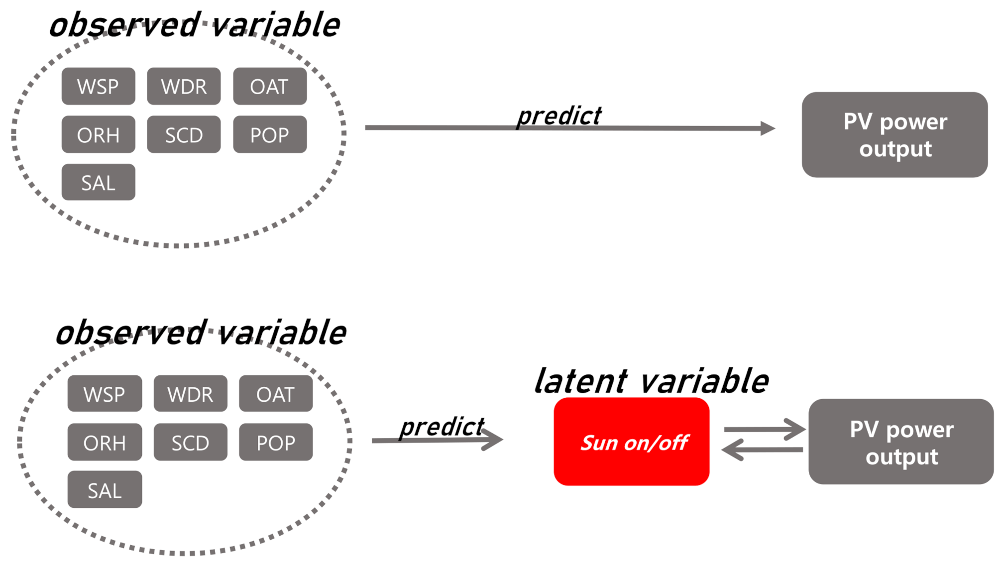
16] and misses a few important variables. For example, a variable that records whether the sun has risen or not is a very important variable in predicting PV power output, but traditional models do not take this into account.
The proposed model proposes a hierarchical probability model that interprets unobserved (but important) variables as latent variables. We propose an algorithm that iteratively predicts latent variable and PV power out from given data.
Figure 1 is a diagram devised to differentiate between the proposed method and the existing approaches.
The paper’s organization is illustrated as follows.
Section 2 introduces the system description and the framework’s prediction models.
Section 3 will explore how the proposed model of the EM algorithm is characterized.
Section 4 will be a discussion of the prediction performances of various machine learning models and proposed algorithms.
Section 5 will include the conclusion.
2. Backgrounds
2.1. PV Generation System
The office buildings with rooftop PV systems in South Korea are operated in micro energy grid (MEG) with other renewable energy resources and energy storage systems (ESS). The geographical location of the buildings is latitude 37°31
N and longitude 127°14
E. The nominal power output capacity of the PV system is 50 kW which consists of 20 parallel strings of 10 series modules with a capacity of 250 W for each as shown in
Figure 2. Each PV panel is positioned east of south-facing with an angle of 20 degrees from the roofline.
The grid-connected PV systems measure not only PV-related data but historical weather information with weather sensors. All measured parameters were stored in the building energy management system (BEMS) every one hour. The used data period was 1st of November 2016 to 31st of August 2017 (12 months) with hourly intervals. For instance, almost 70% of collected data are used for training and the model predicts hourly PV power output in a day-ahead (24 h) for the rest of the dataset.
2.2. Online Weather Forecasting Dataset
The online weather forecasting data are used to suggest a day-ahead real prediction model obtained from Korea meteorological administration (KMA) and Korea astronomy and space science institute (KASI). The weather forecasting information is provided in 3-h intervals by after tomorrow with online service in XML form and KASI offers solar altitude by the hour. However, there is no way to use historical data for PV forecasting. Thus, this paper gets the data by crawling and interpolates data in the one-hour interval.
The seven weather elements were used as predictors, which were pre-processed at 1-h intervals: wind speed (WSP), wind direction (WDR), outdoor air temperature (OAT), relative humidity (ORH), sky condition (SCD), probability of precipitation (POP), solar altitude (SAL).
Table 1 describes the characteristics of the used weather forecasting datasets.
2.3. Prediction Model Description
In this study, the prediction performance of PV power output was compared commonly used prediction models such expectation-maximization (EM), artificial neural network (ANN), support vector machine (SVM), random forest(RF), classification and regression tree (C&RT), Chi-squared automatic interaction detection (CHAID).
Table 2 presents key hyperparameters of PV power output prediction models.
The ANN is a network composed of artificial neurons or nodes which emulate the biological neurons. This network is made up of input and output layers of processing units identified as nodes that are interconnected via one or more ‘hidden’ layers which are dictated by the numbers of independent and dependent variables sequentially. In this study, a typical feed-forward neural network (FFNN) is used which trained only forward direction with information.
The RF is an ensemble-learning algorithm that combines a large set of regression trees. Each of the classification trees is built with a bootstrap sample of the data. Thus, RF uses bootstrap aggregation, a successful approach for combining unstable learners, and random variable selection for tree building.
The CART is an effective binary recursive partitioning algorithm that can automatically search the optimal decision tree and feature selection with the classification effect of the features at each node. CART built the tree by recursively splitting the variable space based on the impurity of the variables to determine the split till the termination condition is met.
The CHAID is a single variable prediction one which is a dependent variable, the other variables are referred to as the predictor variables. CHAID is an iterative technique that determines the most effective method given the dataset. Child nodes are created by splitting the subsets of the space repeatedly. This is done to the whole dataset to construct CHAID. A merger is done between any allowable pairs of categories of the predictor variable to ascertain the best split at each node.
The SVM is a classification model based on statistical learning theory and structural risk minimization principle. The SVM, a classification model, was established on the statistical learning theory and the structural risk immunization principle. SVM operates as a non-linear mapping, renovating the new training data into a higher dimension. With the new dimension, the SVM examines the linear optimal separating hyper-plane.
3. Proposed Method
Machine learning models involve a heavy computational burden, which is not appropriate for the circumstances of Korean historical weather station data. In contrast to previous studies using machine learning models, this research uses the expectation-maximization (EM) algorithm [
17]. There are numerous applications of the EM algorithm with the identification of missing data in aggressive models and hidden variables of each state [
18]. Irregular performance with missing gathered data in industrial processes happens regularly. Kalyani et al. [
19] suggested an EM algorithm setting for removal of outliers in irregular data. The EM algorithm has been applied in various ways to incomplete data with missing values. Also, Deng et al. [
14] dealt with a Bayesian framework using the EM algorithm to reduce uncertainty errors in soft lab data. However, there is no research that applies the EM algorithm to the regression and prediction of specific values, and it is applicable to other industrial systems to handle various latent variables. Also, modeling of the EM algorithm has no hyper-parameters for tuning compared to other machine learning methods and consumes a lot of time and domain knowledge randomness. With similar circumstances as the previous research mentioned above, predicting the weather data of Korean weather stations is incomplete. So, this research applies the EM algorithm to conduct PV prediction. In figuring out the input features of data, the sky condition would have the lowest correlation with power generation. Also, this research considers the sky condition as a latent variable to estimate PV output. Although the sky condition is not an important variable, it is difficult to estimate in weather forecasting data due to the weather forecasting comprising four different levels of cloudiness. For this reason, there is a disadvantage that the performance of the previous model varies greatly depending on sky condition measurement accuracy. To avoid those drawbacks, the sky condition is considered a latent variable among other features and the EM algorithm is applied to jointly estimate the sky condition and PV output. In addition to correlation analysis of input data, the input of probabilities of precipitation and sky conditions are very correlated with the values shown as
Table 3. The correlated values do not affect the prediction results. Thus, this research uses the POP input variable instead using both of POP and SCD input variables shown as
Figure 3.
Our goal was to construct a model that can predict pvoutput. The pvoutput means the amount of power generated from sunlight, which is affected by various weather conditions. We observed an hourly rate of electricity production from 01:00 on 21st of November, 2016 to 23:00 on 26th of August, 2017, yielding 6504 observations. Let these values as , so is a vector. Further, define the weather conditions that affect as . The design matrix is composed of observations of the following five weather conditions, thus is a matrix.
The value of
was obtained from Korea Meteorological Administration (
https://data.kma.go.kr). Predicting
based on
seems very reasonable at first glance, but the result is somewhat inaccurate. The reason for this is that the most important factor in predicting
is whether the sun is on or off. If the sun does not rise, the amount of power produced would only be zero, even though all of the values of
(
wind speed, ... , solar altitude) would meet the perfect conditions for power generation.
For this reason, our study introduces a latent variable which indicates the presence of the sun. Like , is a vector of length 6504 and means that there is no sun at time i and means the sun exists at time i. Note that is not a simple variable to distinguish day and night at the time i. That is, it is not true that the solar altitude at the time i implies . For example, during rainy daylight, the solar altitude is positive but .
To consider the effects of
, consider the following model:
and assume that (1)
where
, (2)
where
, and (3)
. In here
,
, and
is the
th element of
. The parameter
controls the average value of
, which means the probability that the sun exists at the
ith time. Above the model,
is the power output when
, and we assume that it can be modeled by simple linear regression. The
is the power output when
, and we assume that it is always zero. For each
i, we observe
rather than
. Thus,
is the observed data and
is the complete data. To handle this missing problem, we adapt the EM algorithm.
Let
. The likelihood of complete data is as follows:
where
and
Here, is the Dirac delta function and .
In this step, we need to calculate the conditional expectation
The most important part of the calculation of
is the calculation of
which is a function of
where
is current estimate value of
. By definition of conditional expectation,
can be expressed as
Note that
is always 0 when
, otherwise
is always 1 due to the characteristics of the delta function. Thus,
where
is the indicator function. This means that
is not a function of
, so
can be obtained by repeating E-step and M-step only once. This ensures very fast convergence.
Let us differentiate
by
.
Note that
since
is constant of
. The term
can be expressed as follows:
From
and
we can easily check that
is equivalent to
where
. Note that Equation (
1) is an interpretable and reasonable condition. Here,
m can be interpreted as the number of observations when the sun rises and we define
as the probability of the sun rising at each observation. Therefore, Equation (
1) means the sum of probabilities of sunrise equals to the number of observations that actually sun was up.
Now let us differentiate
by
.
The left one can be calculated as
Since
is a
vector,
is a
matrix such that
thus,
can be expressed as follows:
Similarly, one can easily check that
Note that
and
can be expressed as
where
and
. Here,
can be considered as another design matrix defined except for the observation where
is zero. By introducing the
, we can express
as
Now, let us focus on the term
. This term can be calculated as
Using
and
, we get
Observe
where
is an
vector such that
. Similarly, one can check that
where
is an
vector with
. Thus,
Combining Equations (
2) and (
3), we obtain
Therefore the last step is to solve the following equations.
To solve (
4), we propose the following Algorithm 1.
| Algorithm 1 Proposed algorithm for prediction of PV power output |
- 1:
Get m and . - 2:
Initialize and as and and set . - 3:
- 4:
- 5:
- 6:
Repeat 3–5 until convergence.
|
4. Results
This research conducts various machine learning models and probabilistic models to predict PV generation included in
Section 2 and
Section 3. The analysis was conducted from largely the following three viewpoints.
4.1. Overall Performance Comparison
In this section, the overall performances of five machine learning models and the proposed method are compared.
Figure 4 shows the goodness-of-fit through
when each of 5 months-8 months was set as a training set. The x-axis of each figure is the actual data, and the y-axis is the estimated values. Therefore, it can be interpreted that the more the points are concentrated near the straight line, the more excellent the models are. The degree to which the points are concentrated near the straight line is indicated through
, and the higher the value of
, the better the fit of the model.
When 6 months and 7 months were set as training sets, respectively, the ANN model showed the highest fits, and the value at this time was 0.75. However, when trained on data for 5 months and 8 months, respectively, the ANN model did not show the same high fits as with 6 and 7 months. In addition to the ANN method, the proposed method EM algorithm showed high fits. EM showed evenly good performances for 5–8 months and has the advantage of showing relatively uniform performances compared to the ANN method. Other methods generally have poorer fits compared to EM and ANN.
In analyses thereafter, all training sets were set to 7 months. The reasons why the training sets were set to 7 months are (1) that our target model, ANN, is the setting that shows the best performance, and (2) that if the methods learn for 7 months, the methods will learn until June and given that the rainy season in Korea is June-August, learning June, which is one month in the rainy season, was thought to be appropriate.
Figure 5 is a box plot of errors when 7 months was set as the training set. The box plot is meaningful for comparing the overall performances of the models, but it is not informative. When evaluating the prediction performance of solar electric energy, the point that is worthy of attention is the fit between 8:00 and 17:00 because this is the time zone in which electric energy is mainly produced. The analysis in this section gives no information about the fit for the time we are interested in.
4.2. Analysis of Model Performances by Time
To overcome the limitations of the analysis described in
Section 4.1, the performances of the model should be reanalyzed by time zone.
Figure 6 shows the comparison of the fits of individual models by time.
An overall feature is the outliers of the errors from 7:00 to 17:00. This coincides with the time when the sun is up. The differences in errors between the time when the sun is up and the time when the sun is not up are very intuitive because when the sun is not up, the electric energy production can be set to zero. Except for the SVM model, it can be seen that most of the models well-adjusted the electric energy production to 0 during the time when the sun was up. All models generally have large errors during the time. In particular, such errors are outstanding between 10:00 and 14:00. Since this is the time when the sunlight is the strongest in a day, it is more difficult to predict accurate electric energy production.
A salient feature is the outliers of the errors between 7:00 and 17:00. The outliers are expressed as points that deviated from the box plot. SVM has the least number of outliers followed by the EM algorithm. The fact that a model has many outliers means that there are many points where the prediction by the model deviates greatly because the variance of the model is large. Therefore, models with many outliers are suspected of overfitting. Other models’ outliers are very large from 15:00 to 17:00.
In terms of performance stability, the EM algorithm and SVM are excellent. However, SVM has a disadvantage in that the overall fitting is poor. In addition, the fitting of SVM is much poorer compared to other models when electric energy production is zero. ANN has a good overall fit but has a weakness of unstable performances in certain time zones.
4.3. Analysis of a Certain Day after Magnifying and Refocusing
In this section, we compare the performances of EM and ANN-based on a certain day. In addition, we refocus on the overfitting issue of ANN more clearly. ANN has an issue of overfitting with various training datasets. The top row of
Figure 7 shows that both EM and ANN predicting PV outputs. The bottom row of
Figure 7 enlarges among EM, ANN, and real values of PV from 28th of June to 3rd of July.
In
Figure 7, the results of ANN and EM are represented in blue and red, respectively. Actual values are expressed in gray shades. During the periods of rainy days, EM has more stable predicting results compared to ANN. ANN has no mountain-shaped fit results like the overfitting results. The results of EM are explainable to predict the PV outputs. Especially, from 28th of June to 29th of June, and 2nd of July, the predicted values of ANN are very volatile, and if a real-time prediction result was required, the ANN’s results are useless. The results of EM are also the same in that it is not suitable for the periods, but EM yields explainable mountain-shape results. Without the sudden rain, EM would have been a very good fit.
Considering the overall aspects, the advantages of EM can be summarized as follows.
Goodness of Fit: Overall results of the fit are excellent with ANN (deep neural network).
Stability: There is little difference in performance between performances based on values.
Explainable model: It is an interpretable model as described before.
Lightness: The model is light and estimates very fast. The reason is that is not the function of .
Avoid overfitting issue: It is more free from the overfitting issue than other complex models (ANN).
No hyperparameter: There are no separate hyperparameters to be set to train the model. This means that it is easy to use overall aspects with no expertise.


