Optimal Design and Analysis of Sector-Coupled Energy System in Northeast Japan


Abstract
:1. Introduction
2. Methods
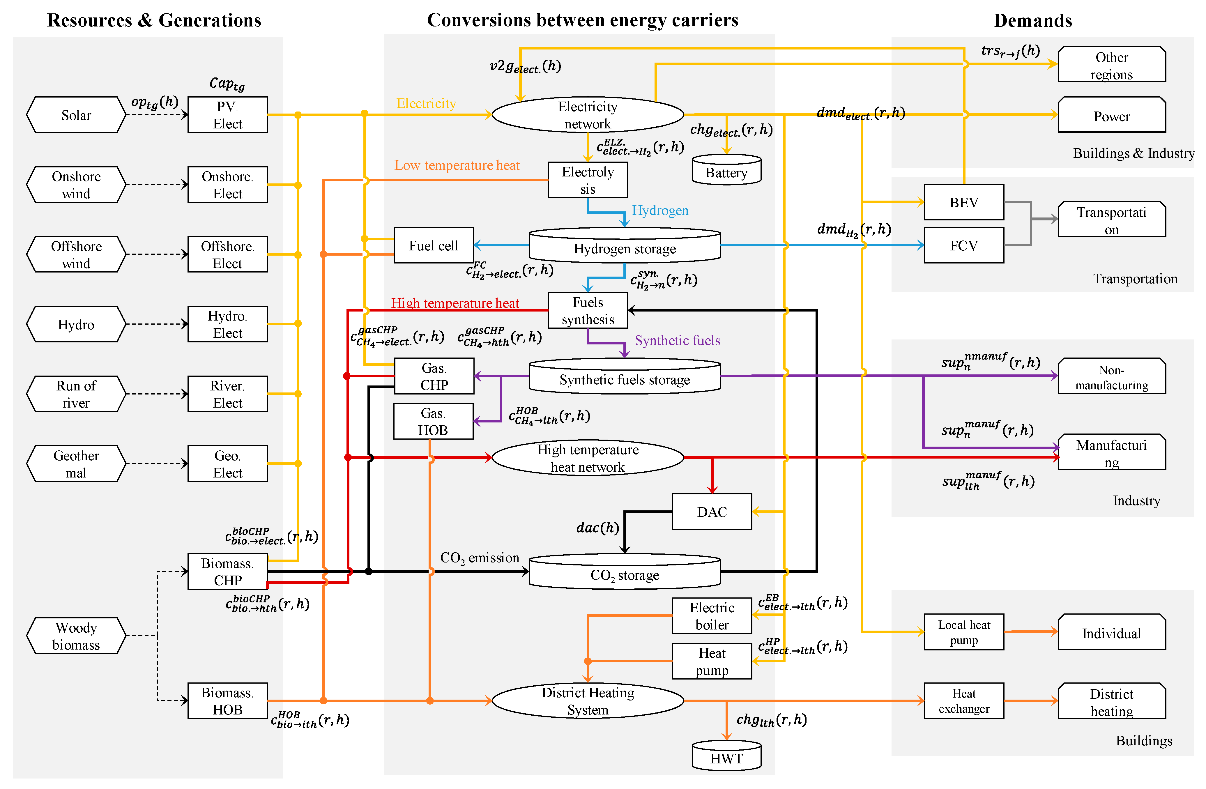
2.1. System Configuration of the Sector-Coupled Energy System
2.2. Optimization Model
2.3. Input Data and Assumptions
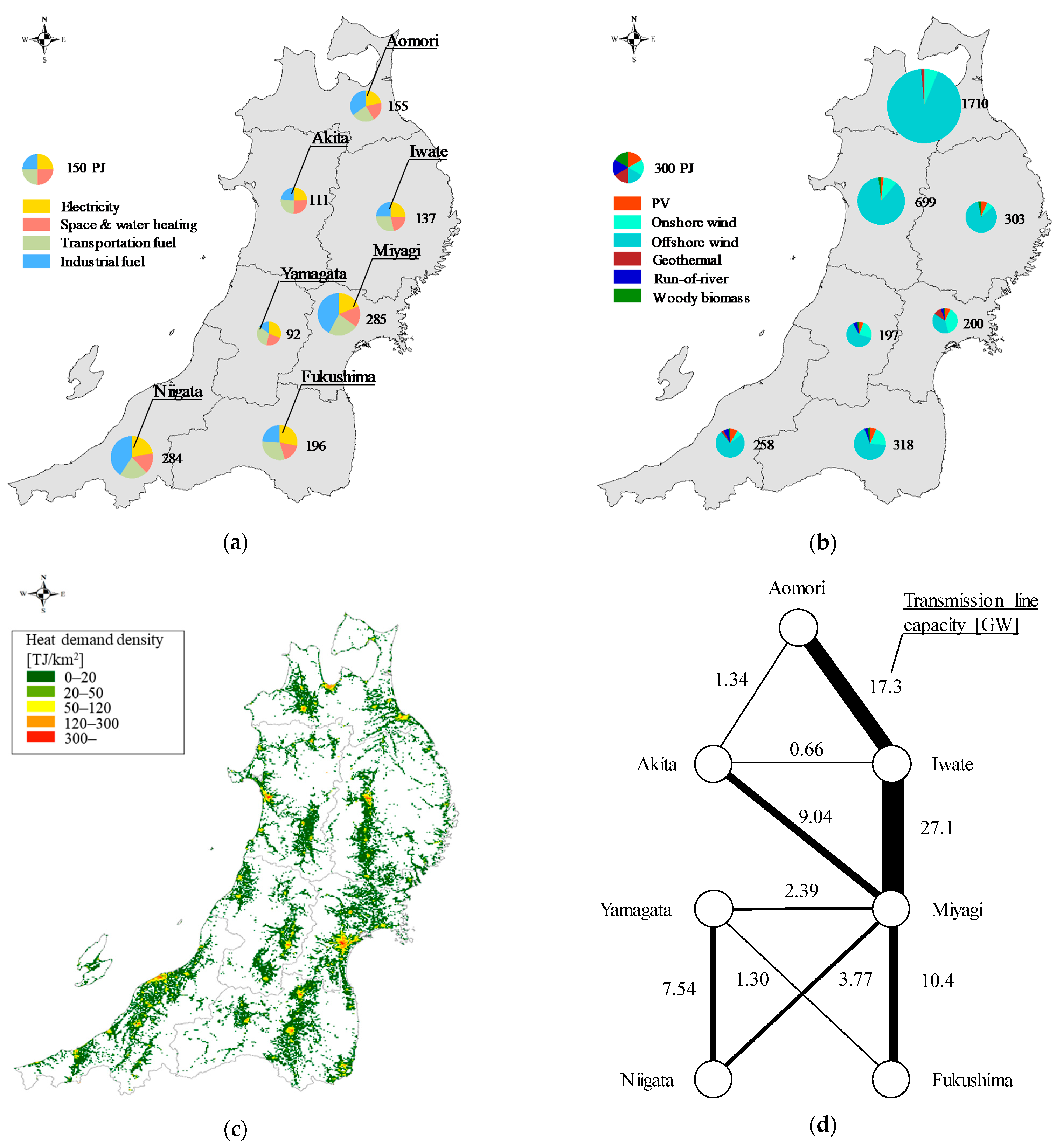
2.3.1. Target Region
2.3.2. Estimation of Energy Demands
2.3.3. Estimation of Energy Supply from Renewable Energy
2.3.4. Technical and Economic Parameters
3. Results
3.1. Scenario Setting
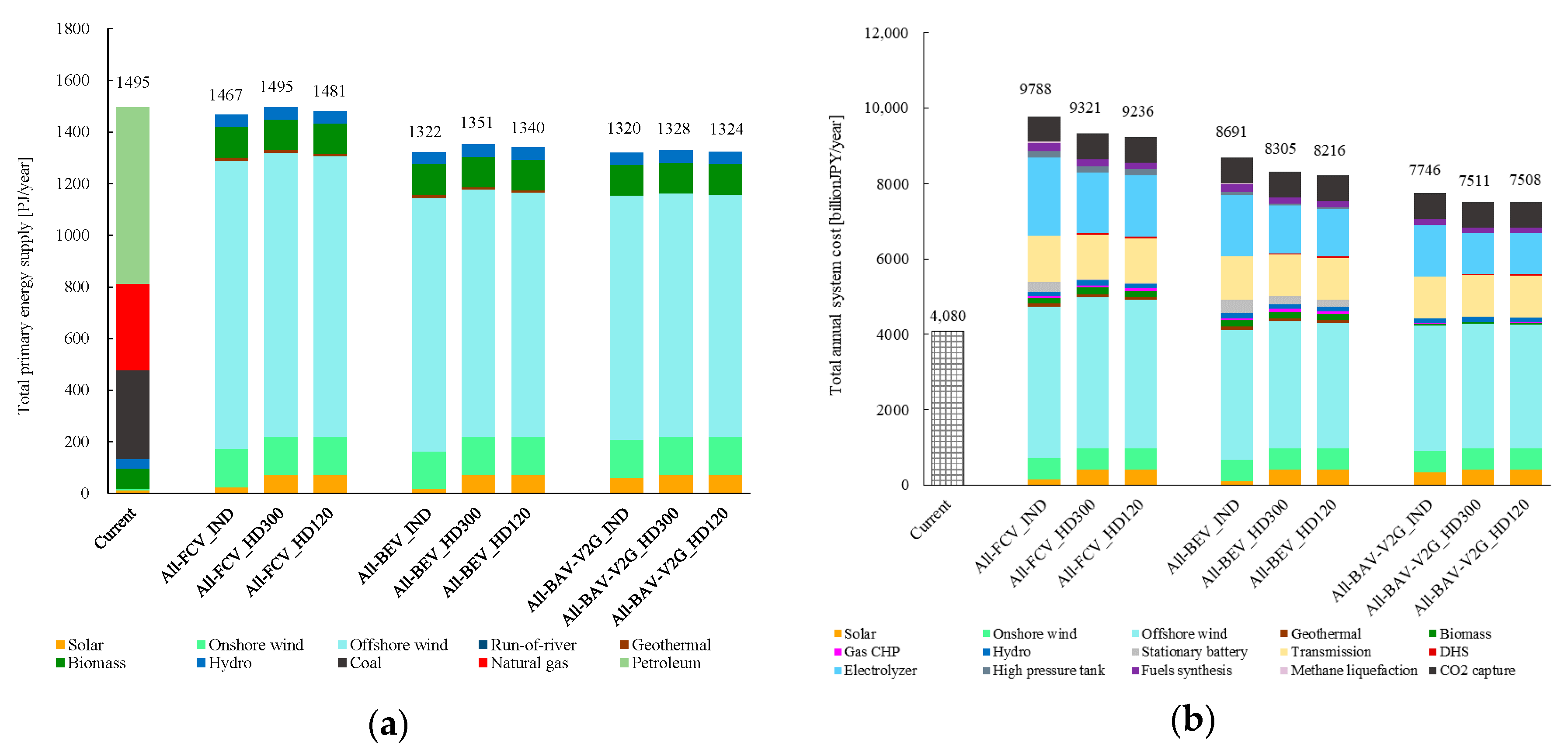
3.2. Comparison of Total Primary Energy Supply (TPES) and Total Annual System Cost in Each Scenario
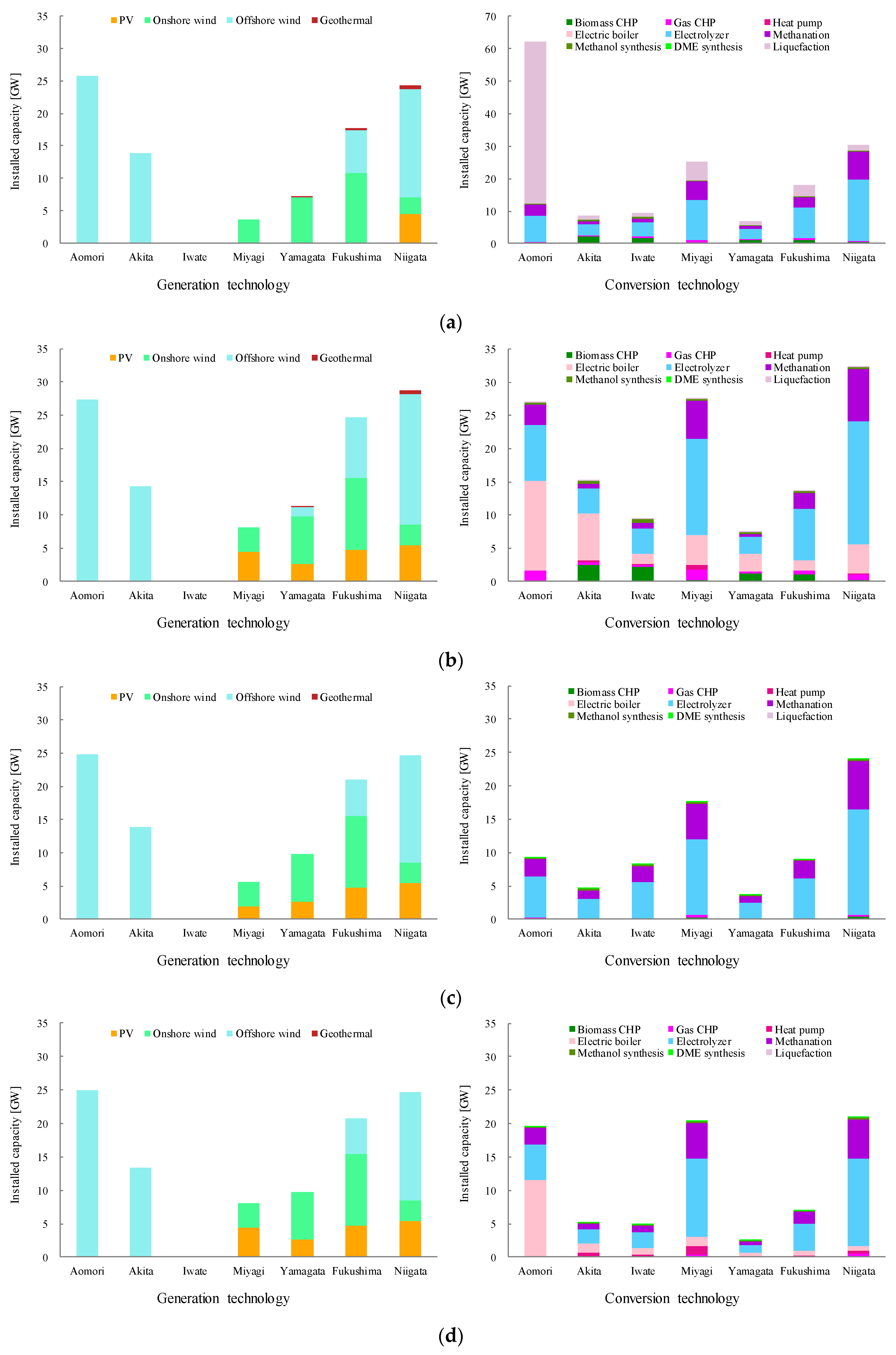
3.3. Installed Capacity of Each Technology
3.4. Hourly Energy Balances in the Sector-Coupled Energy System
3.5. Comparison with the Current Energy System
4. Discussion
4.1. Toward Implementation of the Sector-Coupled Energy System in Japan
4.2. Possible Improvements
5. Conclusions
- The total primary energy supply will decrease, but the amount of generation may be required to be about four times the current amount. In Japan, it can be expected that it would be necessary to introduce more than 35 times the current amount of renewable energy to realize decarbonization by renewable resources. The annual total system cost of the designed energy systems increases from 1.8 to 2.4 times the current level.
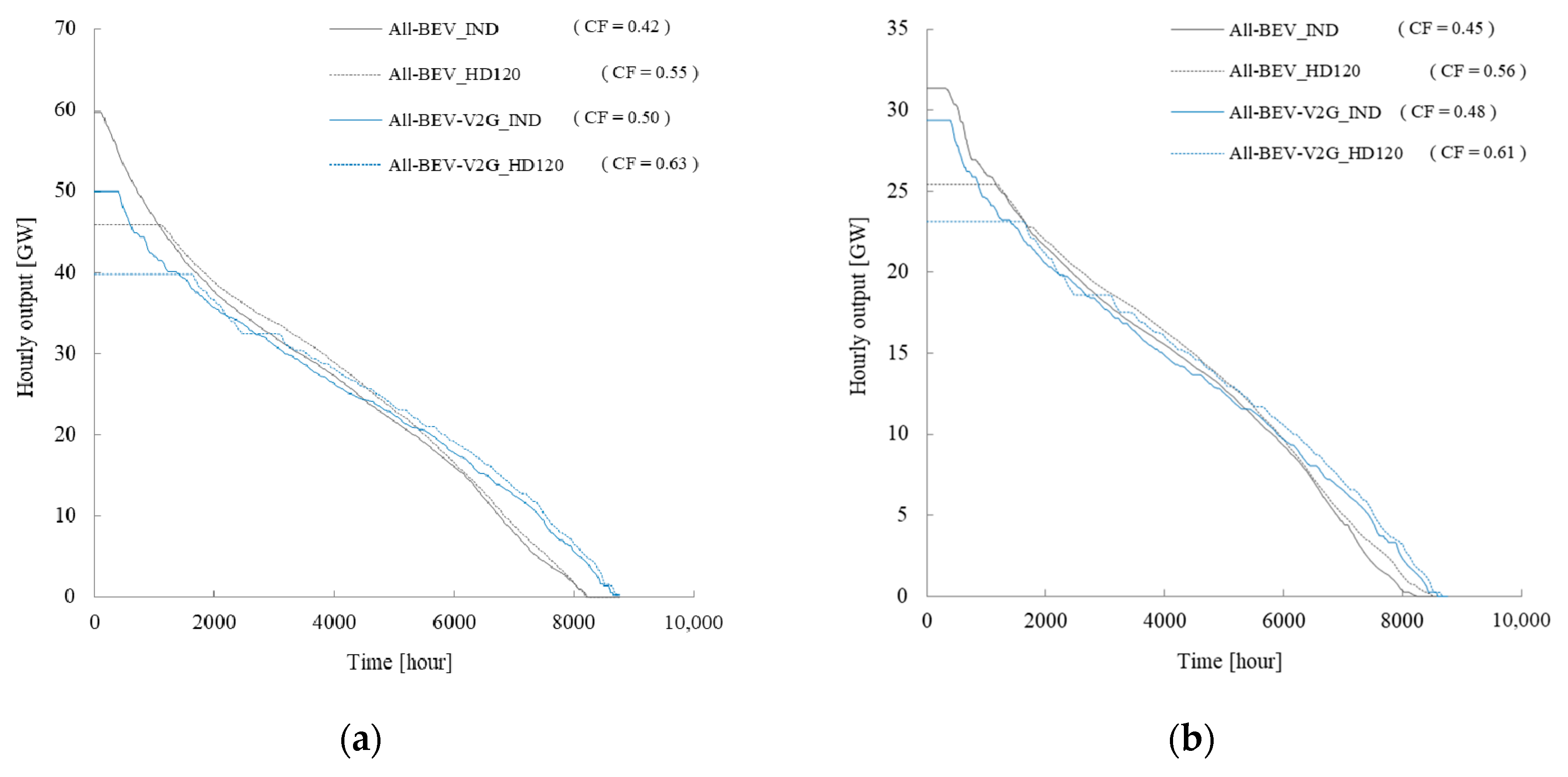
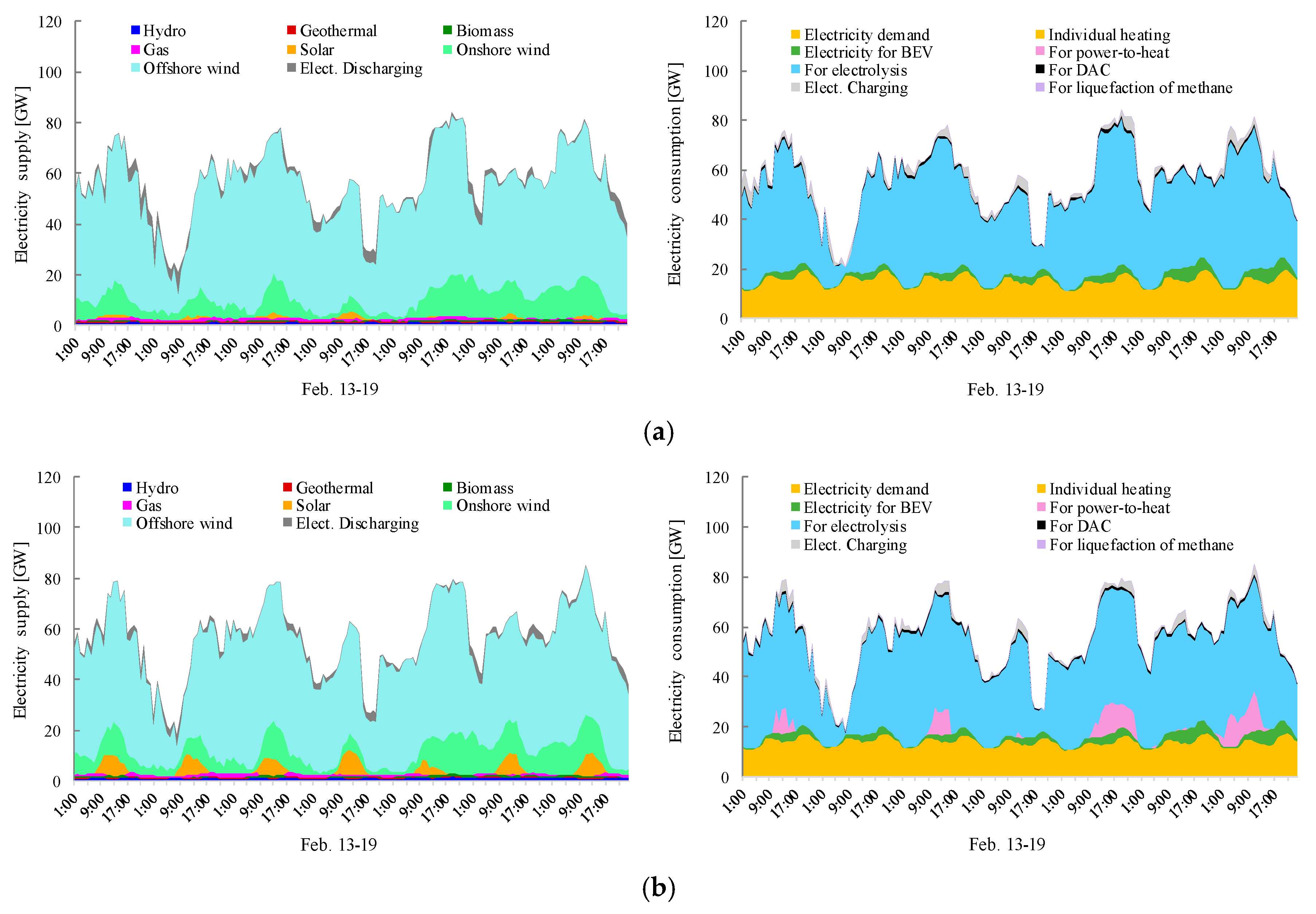
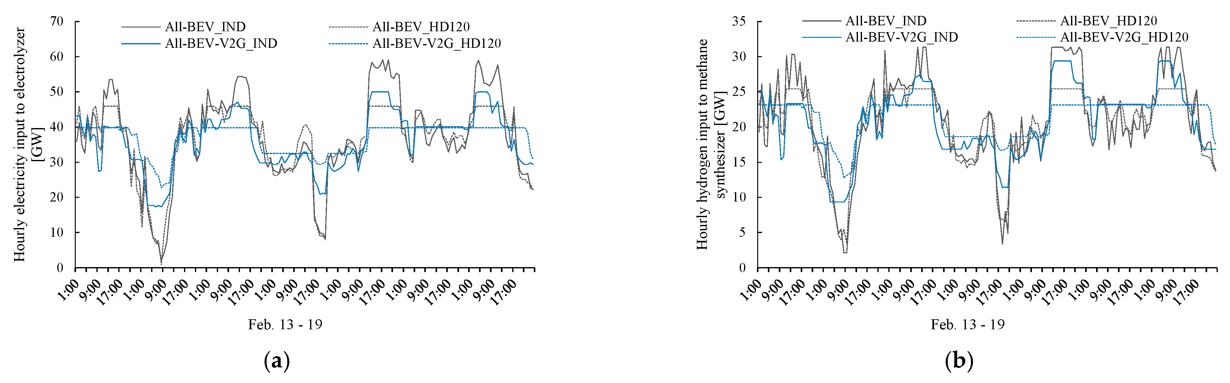
- The annual system cost of the scenario introducing district heating systems and using electric vehicles for V2G is minimal. As a result of the analysis of hourly energy balance, it becomes clear that the peak cut effect by P2H and the peak shift effect by V2G result in the leveling of the electrolyzer, and fuel synthesizer’s output improves the capacity factor and reduces the introduction capacity. It is necessary to utilize electric vehicles by V2G and provide policy support for district heating systems to reduce costs.
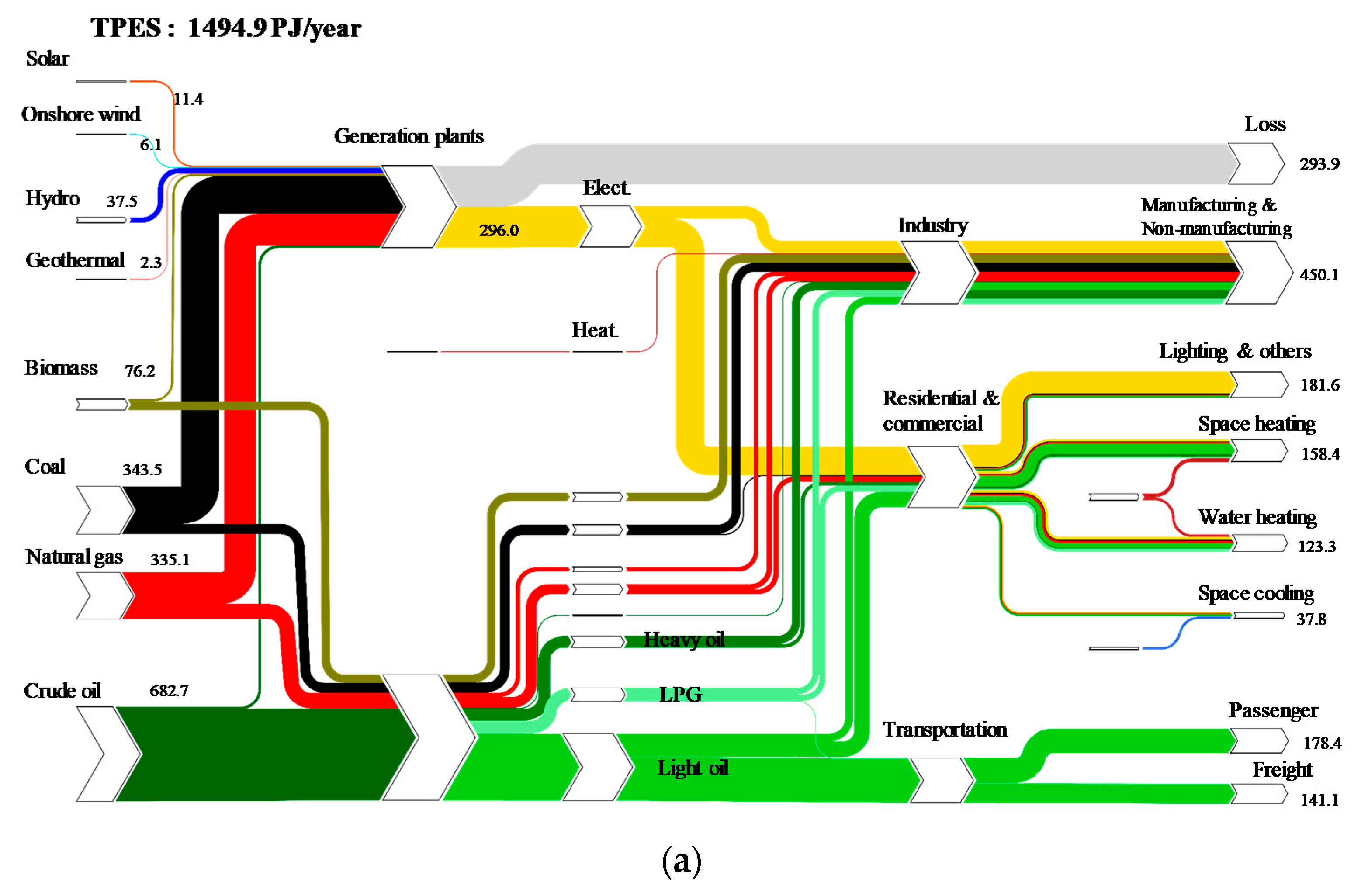
- From the analysis of energy flow, it is confirmed that in the optimization model proposed in this study, the synthetic fuels supplied to the industrial sector have a considerable influence on the amount of power generation.
- There is a concern that the capacity of storage batteries and energy conversion technologies will increase to cope with the peak of PV. In areas where the industrial energy share is high, P2H and V2G may help reduce the cost of synthetic fuels. In addition, P2G should be mainly aimed at producing synthetic fuels, not flexibility.
- To reduce the amount of renewable energy required, it is necessary to reduce the energy demand in the industrial sector and electrify the energy demand. To reduce energy demand in the industrial sector, it is important to transform lifestyles that were not considered in this study into sustainable ones.
- For future research, it is important to incorporate more technologies, improve the model’s accuracy with reliable data, and model the optimization on the demand side. It is also required to apply the model to all regions of Japan.
Author Contributions
Funding
Conflicts of Interest
Nomenclature
| Sets | |
| Hour | |
| Link of transmission line | |
| Other regions | |
| Synthetic fuels (methane, methanol, DME) | |
| Technology | |
| Conversion technology | |
| Generation technology | |
| Region | |
| Indices | |
| Total capital and O&M costs (million JPY/year) | |
| Total carbon capture costs (million JPY/year) | |
| Total costs for methane liquefaction (million JPY/year) | |
| Total annual system costs (million JPY/year) | |
| Total transmission costs (million JPY/year) | |
| , , | The total amount of captured CO2 (t-CO2/year) |
| Primary energy supply to CHP plants by woody biomass (GW) | |
| Primary energy supply to CHP plants by methane (GW) | |
| , | The amount of electricity stored in batteries (GWh) |
| The amount of hydrogen stored in high-pressure tanks (GWh) | |
| The amount of low-temperature heat stored in hot water tanks (GWh) | |
| , . | The amount of methane stored in gas and liquid state (GWh) |
| The amount of synthetic fuel stored in fuels tanks (GWh) | |
| Woody biomass stock (GWh) | |
| The amount of CO2 stored in tanks (t-CO2) | |
| Total allowed maximum vehicle-to-grid outputs (GW) | |
| Parameters | |
| Photovoltaic panel area (m2/kW) | |
| Overnight capital cost (million JPY/GW) | |
| Transmission line capacity (GW) | |
| The storage capacity of a battery in a vehicle (GWh/vehicle) | |
| CO2 demands for fuels synthesis (t-CO2/GWhydrogen) | |
| , | The carbon emission factor of woody biomass and methane (t-CO2/GWh) |
| Capital recovery factor (-) | |
| Annual fuels demand in the manufacturing industry (GWh) | |
| Annual fuels demand in the non-manufacturing industry (GWh) | |
| Electricity consumption by BEV driving (GW) | |
| Hourly electricity demand (GW) | |
| Hourly hydrogen demand (GW) | |
| Hourly low-temperature heat demand (GW) | |
| Desirable depth of discharge for stationary battery (-) | |
| , | Electricity consumption for DAC (GWh/t-CO2) |
| High-temperature heat consumption for DAC (GWh/t-CO2) | |
| Electricity consumption from methane liquefaction (GWh/GWh) | |
| Interest rate (-) | |
| A lifetime of technology (year) | |
| The number of vehicles (vehicle) | |
| The hourly output from renewables’ generation technology (GW/GW) | |
| Output ratio to battery capacity (-) | |
| Percentage of traveling vehicles (-) | |
| Annual utilization potential of woody biomass (GWh) | |
| Installation potential of renewables’ generation (GW) | |
| Solar radiation (MJ/m2/h) | |
| , | Desirable state of charge for battery in BEV (-) |
| Unit capital and O&M cost of technology t (million JPY/GW) | |
| The annualized unit cost of capital (million JPY/GW/year) | |
| , , | The unit cost of carbon capture from CHP plants and DAC (million JPY/t-CO2) |
| The annualized unit cost of fuel (million JPY/GW/year) | |
| Unit cost for methane liquefaction (million JPY/GWh) | |
| The annualized unit cost of capital, O&M, and fuel (million JPY/GW/year) | |
| The unit cost of electricity transmission (million JPY/GWh) | |
| The available daily factor of vehicles (-) | |
| Average trips per vehicle (-) | |
| Vehicle participation rate in V2G (-) | |
| , | Specific electrical power loss for CHP (-) |
| Energy conversion efficiency (-) | |
| , | Electrical efficiency of CHP plants (-) |
| The efficiency of battery storage (-) | |
| , | Carbon capture efficiency in CHP plants (-) |
| Heat exchange efficiency (-) | |
| The efficiency of hot water tank storage (-) | |
| The efficiency of heat recovery from fuel synthesizers (-) | |
| , | The efficiency of photovoltaic panel and power conditioner (-) |
| Allowed maximum vehicle-to-grid outputs per vehicle (GW) | |
| , | The power-to-heat ratio of CHP in back-pressure operation (-) |
| Decision variables | |
| Energy conversion from x into y by technology tc (GW) | |
| The capacity of technology t (GW) | |
| , | Electricity charging to stationary batteries (GW) |
| Low-temperature heat charging to hot water tanks (GW) | |
| CO2 captured by DAC (t-CO2) | |
| Heat recovery from electrolyzer (GW) | |
| Heat recovery from fuel cell (GW) | |
| The amount of liquefied methane (GW) | |
| Synthetic fuels supply to (non)manufacturing industry (GW) | |
| High-temperature heat supply to manufacturing industry (GW) | |
| The amount of electricity transmitted between regions (GW) | |
| Electricity discharged from BEV to the electrical grid (GW) |
References
- Lund, H.; Østergaard, P.A.; Connolly, D.; Mathiesen, B.V. Smart Energy, and Smart Energy Systems. Energy 2017, 137, 556–565. [Google Scholar] [CrossRef]
- Connolly, D.; Lund, H.; Mathiesen, B.V. Smart Energy Europe: The Technical and Economic Impact of One Potential 100% Renewable Energy Scenario for the European Union. Renew. Sustain. Energy Rev. 2016, 60, 1634–1653. [Google Scholar] [CrossRef]
- Niemi, R.; Mikkola, J.; Lund, P.D. Urban Energy Systems with Smart Multi-Carrier Energy Networks and Renewable Energy Generation. Renew. Energy 2012, 48, 524–536. [Google Scholar] [CrossRef]
- Thellufsen, J.Z.; Lund, H. Cross-Border versus Cross-Sector Interconnectivity in Renewable Energy Systems. Energy 2017, 124, 492–501. [Google Scholar] [CrossRef]
- Syranidou, C.; Linssen, J.; Stolten, D.; Robinius, M. Integration of Large-Scale Variable Renewable Energy Sources into the Future European Power System: On the Curtailment Challenge. Energies 2020, 13, 5490. [Google Scholar] [CrossRef]
- Tremel, A.; Wasserscheid, P.; Baldauf, M.; Hammer, T. Techno-Economic Analysis for the Synthesis of Liquid and Gaseous Fuels Based on Hydrogen Production via Electrolysis. Int. J. Hydrogen Energy 2015, 40, 11457–11464. [Google Scholar] [CrossRef]
- Götz, M.; Lefebvre, J.; Mörs, F.; McDaniel Koch, A.; Graf, F.; Bajohr, S.; Reimert, R.; Kolb, T. Renewable Power-to-Gas: A Technological and Economic Review. Renew. Energy 2016, 85, 1371–1390. [Google Scholar] [CrossRef] [Green Version]
- Guilera, J.; Ramon Morante, J.; Andreu, T. Economic Viability of SNG Production from Power and CO2. Energy Convers. Manag. 2018, 162, 218–224. [Google Scholar] [CrossRef]
- Ikäheimo, J.; Pursiheimo, E.; Kiviluoma, J.; Holttinen, H. Role of Power to Liquids and Biomass to Liquids in a Nearly Renewable Energy System. IET Renew. Power Gener. 2019, 13, 1179–1189. [Google Scholar] [CrossRef]
- Varone, A.; Ferrari, M. Power to Liquid and Power to Gas: An Option for the German Energiewende. Renew. Sustain. Energy Rev. 2015, 45, 207–218. [Google Scholar] [CrossRef] [Green Version]
- Blanco, H.; Nijs, W.; Ruf, J.; Faaij, A. Potential of Power-to-Methane in the EU Energy Transition to a Low Carbon System Using Cost Optimization. Appl. Energy 2018, 232, 323–340. [Google Scholar] [CrossRef]
- Nastasi, B.; Mazzoni, S.; Groppi, D.; Romagnoli, A.; Astiaso Garcia, D. Solar power-to-gas application to an island energy system. Renew. Energy 2021, 164, 1005–1016. [Google Scholar] [CrossRef]
- Bloess, A. Impacts of Heat Sector Transformation on Germany’s Power System through Increased Use of Power-to-Heat. Appl. Energy 2019, 239, 560–580. [Google Scholar] [CrossRef]
- Obara, S.; Ito, Y.; Okada, M. Electric and Heat Power Supply Network of Hokkaido in Consideration of the Leveling Effect by a Wide-Area Interconnection of Wind-Farm and Solar-Farm. Trans. JSME 2017, 83. [Google Scholar] [CrossRef] [Green Version]
- Ashfaq, A.; Kamali, Z.H.; Agha, M.H.; Arshid, H. Heat Coupling of the Pan-European vs. Regional Electrical Grid with Excess Renewable Energy. Energy 2017, 122, 363–377. [Google Scholar] [CrossRef] [Green Version]
- Taljegard, M.; Göransson, L.; Odenberger, M.; Johnsson, F. Impacts of Electric Vehicles on the Electricity Generation Portfolio—A Scandinavian-German Case Study. Appl. Energy 2019, 235, 1637–1650. [Google Scholar] [CrossRef]
- Child, M.; Nordling, A.; Breyer, C. The Impacts of High V2G Participation in a 100% Renewable Åland Energy System. Energies 2018, 11, 2206. [Google Scholar] [CrossRef] [Green Version]
- Brown, T.; Schlachtberger, D.; Kies, A.; Schramm, S.; Greiner, M. Synergies of Sector Coupling and Transmission Reinforcement in a Cost-Optimised, Highly Renewable European Energy System. Energy 2018, 160, 720–739. [Google Scholar] [CrossRef] [Green Version]
- Bailera, M.; Lisbona, P.; Peña, B.; Romeo, L.M. A review on CO2 mitigation in the iron and steel industry through power to X processes. J. CO2 Util. 2021, 46. [Google Scholar] [CrossRef]
- IEA. World Energy Balances 2018; IEA: Paris, France, 2018. [Google Scholar] [CrossRef]
- Takita, Y.; Furubayashi, T.; Nakata, T. Development and Analysis of an Energy Flow Considering Renewable Energy Potential. Trans. JSME 2015, 81. [Google Scholar] [CrossRef]
- Lehner, M.; Tichler, R.; Steinmüller, H.; Koppe, M. Power-to-Gas: Technology and Business Models; Springer: Berlin/Heidelberg, Germany, 2014. [Google Scholar] [CrossRef]
- Lund, H.; Werner, S.; Wiltshire, R.; Svendsen, S.; Thorsen, J.E.; Hvelplund, F.; Mathiesen, B.V. 4th Generation District Heating (4GDH). Integrating Smart Thermal Grids into Future Sustainable Energy Systems. Energy 2014, 68, 1–11. [Google Scholar] [CrossRef]
- Tohoku Electric Power Co., Inc. Power System Diagram (Primary System). Available online: https://www.tohoku-epco.co.jp/jiyuka/04/5001.pdf (accessed on 4 February 2020).
- Tohoku Electric Power Co., Inc. Normal Operation Capacity Used for Studying System Access of Trunk Transmission Lines in the Region. Available online: https://www.tohoku-epco.co.jp/jiyuka/04/02.pdf (accessed on 4 February 2020).
- Investigation Committee on Electricity Transmission Fee. Changes of Electric Charge and Transmission Fee. Available online: https://www.cao.go.jp/consumer/content/20180105_20160726_takuso_toshin_betu_shiryou.pdf (accessed on 4 February 2020).
- Tohoku Electric Power Co., Inc. Download Past Actual Data. Available online: http://setsuden.tohoku-epco.co.jp/download.html (accessed on 4 February 2020).
- Ministry of Economy, Trade and Industry. Energy Consumption Statistics by Prefecture. Available online: https://www.enecho.meti.go.jp/statistics/energy_consumption/ec002/ (accessed on 4 February 2020).
- E-Stat. Population Census. Available online: https://www.e-stat.go.jp/gis/statmap-search?page=1&type=1&toukeiCode=00200521 (accessed on 4 February 2020).
- Envirolife Research Institute Inc. Annual Household Energy Statistics (2017); Envirolife Research Institute Inc.: Tokyo, Japan, 2019. [Google Scholar]
- Fujii, S.; Furubayashi, T.; Nakata, T. Design and Analysis of District Heating Systems Utilizing Excess Heat in Japan. Energies 2019, 12, 1201. [Google Scholar] [CrossRef] [Green Version]
- Okumura, K.; Ikaga, T.; Kawakubo, S. Development of the Database for Stock and Flow Floor Area of Non-Residential Buildings Classified by Building Use Type and Area. AIJ J. Technol. Des. 2012, 18, 275–280. [Google Scholar] [CrossRef] [Green Version]
- Japan District Heating & Cooling Association. Handbook of District Heating and Cooling Technologies, 4th ed.; Japan District Heating & Cooling Association: Tokyo, Japan, 2013. [Google Scholar]
- Werner, S. District Heating and Cooling. In Reference Module in Earth Systems and Environmental Sciences; Elsevier: Amsterdam, The Netherlands, 2013. [Google Scholar] [CrossRef]
- Ministry of Land, Infrastructure, Transport and Tourism. Automotive Fuel Consumption Survey. Available online: https://www.mlit.go.jp/k-toukei/nenryousyouhiryou.html (accessed on 4 February 2020).
- Uchida, T.; Furubayashi, T.; Nakata, T. Well-to-Wheel Analysis and a Feasibility Study of Fuel Cell Vehicles in the Passenger Transportation Sector. Trans. JSME 2019, 85. [Google Scholar] [CrossRef] [Green Version]
- National Renewable Energy Laboratory. Fuel Cell Buses in U.S. Transit Fleets: Current Status 2018; National Renewable Energy Laboratory: Denver, CO, USA, 2018. [Google Scholar]
- Lee, D.Y.; Elgowainy, A.; Kotz, A.; Vijayagopal, R.; Marcinkoski, J. Life-Cycle Implications of Hydrogen Fuel Cell Electric Vehicle Technology for Medium- and Heavy-Duty Trucks. J. Power Sources 2018, 393, 217–229. [Google Scholar] [CrossRef]
- GoGoEV. Total Charging Record Information. Available online: https://ev.gogo.gs/special/using_report/ (accessed on 4 February 2020).
- Ministry of the Environment. The Study of Basic Zoning Information on Renewable Energy. Available online: https://www.env.go.jp/earth/ondanka/rep/ (accessed on 4 February 2020).
- Japan Meteorological Agency. Download Past Weather Data. Available online: https://www.data.jma.go.jp/gmd/risk/obsdl/ (accessed on 4 February 2020).
- KYOCERA Corporation. Catalog of Solar Power Generating Systems for Public/Industrial Use. Available online: https://www.kyocera.co.jp/solar/support/download/uploads/catalog_kyocera_solar_business_1.pdf (accessed on 17 February 2020).
- Japan Oceanographic Data Center. Coastal Maritime Meteorology Data. Available online: https://www.jodc.go.jp/jodcweb/JDOSS/fixed_wave_station_code_j.html (accessed on 4 February 2020).
- Forestry Agency. Current Status of Forest Resources. Available online: http://www.rinya.maff.go.jp/j/keikaku/genkyou/index1.html (accessed on 4 February 2020).
- Brynolf, S.; Taljegard, M.; Grahn, M.; Hansson, J. Electrofuels for the Transport Sector: A Review of Production Costs. Renew. Sustain. Energy Rev. 2018, 81, 1887–1905. [Google Scholar] [CrossRef]
- Power Generation Cost Verification Working Group. Report on Verification of Power Generation Costs to the Long-Term Energy Supply and Demand Outlook Subcommittee. Available online: https://www.enecho.meti.go.jp/committee/council/basic_policy_subcommittee/mitoshi/cost_wg/pdf/cost_wg_02.pdf (accessed on 17 February 2020).
- Dahl, M.; Brun, A.; Andresen, G.B. Cost Sensitivity of Optimal Sector-Coupled District Heating Production Systems. Energy 2019, 166, 624–636. [Google Scholar] [CrossRef] [Green Version]
- Rubin, E.S.; Davison, J.E.; Herzog, H.J. The Cost of CO2 Capture and Storage. Int. J. Greenh. Gas Control 2015, 40, 378–400. [Google Scholar] [CrossRef]
- Zakeri, B.; Syri, S. Electrical Energy Storage Systems: A Comparative Life Cycle Cost Analysis. Renew. Sustain. Energy Rev. 2015, 42, 569–596. [Google Scholar] [CrossRef]
- David, A.; Mathiesen, B.V.; Averfalk, H.; Werner, S.; Lund, H. Heat Roadmap Europe: Large-Scale Electric Heat Pumps in District Heating Systems. Energies 2017, 10, 578. [Google Scholar] [CrossRef] [Green Version]
- Schmidt, O.; Gambhir, A.; Staffell, I.; Hawkes, A.; Nelson, J.; Few, S. Future Cost and Performance of Water Electrolysis: An Expert Elicitation Study. Int. J. Hydrogen Energy 2017, 42, 30470–30492. [Google Scholar] [CrossRef]
- Energy Technology Systems Analysis Program (ETSAP). Technology Brief P03: Oil and Natural Gas Logistics; International Energy Agency (IEA): Paris, France, 2011; pp. 1–7. [Google Scholar]
- Fasihi, M.; Bogdanov, D.; Breyer, C. Long-Term Hydrocarbon Trade Options for Maghreb Core Region and Europe—Renewable Energy Based Synthetic Fuels for a Net Zero Emissions World. Sustainability 2016, 3, 306. [Google Scholar] [CrossRef] [Green Version]
- Staffell, I.; Brett, D.; Brandon, N.; Hawkes, A. A Review of Domestic Heat Pumps. Energy Environ. Sci. 2012, 5, 9291–9306. [Google Scholar] [CrossRef]
- NISSAN. NISSAN LEAF Web Catalog. Available online: https://www3.nissan.co.jp/content/dam/Nissan/jp/vehicles/leaf/1912/pdf/leaf_1912_specsheet.pdf (accessed on 4 February 2020).
- Tan, K.M.; Ramachandaramurthy, V.K.; Yong, J.Y. Integration of Electric Vehicles in Smart Grid: A Review on Vehicle to Grid Technologies and Optimization Techniques. Renew. Sustain. Energy Rev. 2016, 53, 720–732. [Google Scholar] [CrossRef]
- EPA. Direct Emissions from Stationary Combustion Sources. Energy Econ. 2008, 34, 1580–1588. [Google Scholar] [CrossRef]
- The Institute of Energy Economics, Japan, Japanese Version of Handbook of Japan’s & World Energy & Economic Statistics; The Institute of Energy Economics: Tokyo, Japan, 2019.
- Ministry of Economy, Trade and Industry. Petroleum Equipment Survey. Available online: https://www.enecho.meti.go.jp/statistics/petroleum_and_lpgas/pl006/ (accessed on 4 February 2020).
- Ministry of Economy, Trade and Industry. Gas Business Annual Report; Ministry of Economy, Trade and Industry: Tokyo, Japan, 2018. [Google Scholar]
- Persson, U.; Wiechers, E.; Möller, B.; Werner, S. Heat Roadmap Europe: Heat Distribution Costs. Energy 2019, 176, 604–622. [Google Scholar] [CrossRef]


| BEV | FCV | ||
|---|---|---|---|
| Passenger | Standard-sized | 0.16 | 0.30 |
| Large-sized | 1.19 | 3.54 | |
| Freight | Standard-sized | 0.16 | 0.30 |
| Large-sized | 2.09 | 3.00 |
| Unit | Overnight Cost [JPY] | Fixed O&M Cost [JPY/year] | Lifetime [year] | η [-] | References | |
|---|---|---|---|---|---|---|
| Solar PV | kWel | 294,000 | 6000.0 | 25 | 1.00 | [46] |
| Onshore wind | kWel | 300,000 | 6000.0 | 25 | 1.00 | [46] |
| Offshore wind | kWel | 565,000 | 22,500.0 | 25 | 1.00 | [46] |
| Run-of-river | kWel | 1,000,000 | 171,590.9 | 22 | 1.00 | [46] |
| Biomass-CHP (CCS) | kWel | 250,000 | 7125.0 | 40 | 0.35 | [47,48] |
| Gas-CHP (CCS) | kWel | 112,500 | 3750.0 | 25 | 0.47 | [47,48] |
| Geothermal | kWel | 790,000 | 33,000.0 | 15 | 1.00 | [46] |
| Battery (Li-ion) | kWh | 68,250 | 862.5 | 15 | 0.95 | [49] |
| Biomass-HOB | kWth | 100,000 | 7125.0 | 20 | 1.08 | [47] |
| Hot water tank | kWh | 1125 | 0.0 | 30 | 0.95 | [13] |
| Heat pump in DHS | kWth | 87,500 | 250.0 | 25 | 4.50 | [47,50] |
| Electric boiler | kWth | 8750 | 137.5 | 20 | 0.98 | [47] |
| Gas-HOB | kWth | 7500 | 250.0 | 25 | 1.03 | [47] |
| Electrolyzer (PEM) | kWel | 232,500 | 11,625.0 | 20 | 0.62 | [45,51] |
| High pressured tank | kWh | 16,250 | 0.0 | 20 | 1.00 | [49] |
| Fuel cell | kWel | 405,375 | 3125.0 | 20 | 0.42 | [49] |
| Methanation | kWfuel | 75,000 | 3000.0 | 25 | 0.77 | [45] |
| Methanol synthesis | kWfuel | 125,000 | 5000.0 | 25 | 0.79 | [45] |
| DME synthesis | kWfuel | 125,000 | 5000.0 | 25 | 0.80 | [45] |
| Methane liquefaction | kWfuel | 9533 | 0.0 | 25 | 1.00 | [52] |
| Direct Air Capture | tCO2/year | 28,500 | 1140.0 | 30 | [53] | |
| CO2 tank | tCO2 | 225,000 | 0.0 | 20 | 1.00 | [9] |
| Scenarios | Definition |
|---|---|
| Transportation | |
| All-FCV | All transportation is provided by fuel cell vehicles. |
| All-BEV | All transportation is provided by battery electric vehicles. |
| All-BEV-V2G | All transportation is provided by battery electric vehicles, and the normal-sized vehicle can be used for vehicle-to-grid. |
| Heat demand | |
| IND | All heat demand is met by individual heating. |
| HD300 | DHS is introduced in areas where the heat-demand density is over 300 TJ/km2 |
| HD120 | DHS is introduced in areas where the heat-demand density is over 120 TJ/km2 |
Publisher’s Note: MDPI stays neutral with regard to jurisdictional claims in published maps and institutional affiliations. |
© 2021 by the authors. Licensee MDPI, Basel, Switzerland. This article is an open access article distributed under the terms and conditions of the Creative Commons Attribution (CC BY) license (https://creativecommons.org/licenses/by/4.0/).
Share and Cite
Nagano, N.; Delage, R.; Nakata, T. Optimal Design and Analysis of Sector-Coupled Energy System in Northeast Japan. Energies 2021, 14, 2823. https://doi.org/10.3390/en14102823
Nagano N, Delage R, Nakata T. Optimal Design and Analysis of Sector-Coupled Energy System in Northeast Japan. Energies. 2021; 14(10):2823. https://doi.org/10.3390/en14102823
Chicago/Turabian StyleNagano, Naoya, Rémi Delage, and Toshihiko Nakata. 2021. "Optimal Design and Analysis of Sector-Coupled Energy System in Northeast Japan" Energies 14, no. 10: 2823. https://doi.org/10.3390/en14102823