Article

A Prediction Model for Battery Electric Bus Energy Consumption in Transit

Department of Civil Engineering, McMaster University, JHE-301, Hamilton, ON L8S 4L7, Canada
*
Author to whom correspondence should be addressed.
Energies 2021, 14(10), 2824; https://doi.org/10.3390/en14102824
Submission received: 23 April 2021 / Revised: 4 May 2021 / Accepted: 8 May 2021 / Published: 14 May 2021
(This article belongs to the Topic Exergy Analysis and Its Applications)

Abstract

:
This study investigates the impacts of vehicular, operational, topological, and external parameters on the energy consumption (EC) of battery-electric buses (BEBs) in transit operation. Furthermore, the study develops a data-driven prediction model for BEB energy consumption in transit operation that considers these four parameters. A Simulink energy model is developed to estimate the EC rates and validated using the Altoona’s test real-world data. A full-factorial experiment is used to generate 907,199 scenarios for BEB operation informed by 120 real-world drive cycles. A multivariate multiple regression model was developed to predict BEB’s EC. The regression model explained more than 96% of the variation in the EC of the BEBs. The results show the significant impacts of road grade, the initial state of charge, road condition, passenger loading, driver aggressiveness, average speed, HVAC, and stop density on BEB’s energy consumption, each with a different magnitude. The study concluded that the optimal transit profile for BEB operation is associated with rolling grade and relatively lower stop density (one to two stops/km).

1. Introduction

The transportation system has been contributing to a high share of greenhouse gas (GHG) emissions over the past two decades [1,2] Currently, transportation contributes to approximately 20% of global GHG emissions. In contrast, electricity is a clean source of energy (depending on generation), with the potential of net-zero GHG emissions [3,4]. In most developed countries, electricity generation is being shifted to more clean and renewable sources [5]. Therefore, electric mobility is considered a better alternative to reduce the transportation carbon footprint.
In this respect, the electrification of transportation systems is at the forefront of transportation researchers and transportation agencies. In particular, the bus transit system represents a very proper context to operate electric powertrain technology due to the nature of fixed routes and timely operation [3,6]. Electric bus (e-Bus) transit systems provide avenues to reduce GHG emissions and other advantages such as reducing noise and increasing energy efficiency [7,8]. However, before phasing out diesel buses, it is crucial for governments, transit providers, and utility companies to understand the impact of an all-electric fleet on the existing energy infrastructure [9,10,11,12].
In general, e-buses are classified into two main types: fuel cell e-bus (FCEB), which uses hydrogen fuel cells to generate energy on board for the electric motor; and battery e-bus (BEB), which stores the energy on an onboard battery that supplies the electric motor with the required energy [6]. The latter is argued to be more economically feasible due to the relatively lower premium cost and the potential for optimal utilization of the charging process during off-peak times. Besides, BEB technology is mature compared to FCEB, which still faces several technical challenges [6,13].
Implementing BEBs in transit systems requires meticulous infrastructure planning, where each bus route must have an appropriate charging scheme that adheres to the operation schedule [14]. In a BEB transit system, the charging stations and the on-board battery have the highest bearing on the total system cost. The cost of the on-board battery draws about one-third of the overall system cost [10,11,15,16]. Indeed, the state-of-the-art has been focusing on optimizing BEB systems and the associated infrastructure network, to minimize the total cost of ownership associated with BEB implementation in transit systems through the optimal allocation of resources [14,17,18,19]. However, this process depends on an accurate estimation of the consumed energy during operation.
Consequently, predicting an accurate energy consumption (EC) rate is the cornerstone for all BEB studies, including those focusing on fleet optimization, battery capacity/performance, the spatial distribution of infrastructure, component sizing (battery and charger), GHG emissions, and utility grid impact analysis [9,20,21,22,23,24,25].
BEB energy consumption is sensitive to several external operational and topological parameters such as stop density, road grade, driving behaviour, traffic condition, road condition, and temperature, to name just a few [20,26,27,28,29,30]. Furthermore, each transit route exhibits a unique operational and topological profile that contributes to energy demand, and the impact of these external parameters on energy consumption requires detailed modelling.
Although models have been developed in the electric vehicles (EVs) domain to account for such impact, surprisingly, there are a limited number of studies in transit application that relates the energy consumption of BEBs to the operational, topological, and external parameters of transit networks [31]. To better depict the value of such an analysis, one should consider that adjusting the spacing between bus stops or route speed might yield a significant reduction in energy consumption [23].
Therefore, there are valid calls to study the intertwined relationships between the energy consumption of BEBs on the one hand and the vehicular, operational, topological, and external features of transit networks on the other hand. Although some models have been developed to quantify the impact of several parameters of energy model (e.g., speed, rolling resistance, mass, temperature, and frontal area) on the energy consumption [19,29,32], our study contributes to understanding, and predicting, the relationship between the operational, topological, and external features of transit networks and the energy consumption of BEBs. This is curial for policymakers and transit providers to better plan BEB adoption in transit.
Toward that end, the present study aims at quantifying the association between the vehicular, operational, topological, and external parameters of the transit network and the energy consumption of BEBs. More specifically, our goals are to (1) develop a prediction model for BEB energy consumption from the features of transit networks, which in turn (2) is used to inform the design of the optimal transit operation profile that enhances BEB energy utilization.
Following the introduction, a comprehensive review of BEB energy consumption studies is presented in Section 2. Section 3 provides details on the energy consumption simulation model and the model validation. Furthermore, it illustrates the experimental design and the specification of the proposed prediction model. The results of the proposed prediction model are presented in Section 4, followed by a discussion highlighting the practical implications of the proposed model. Lastly, Section 6 concludes the study.

2. BEB Energy Consumption Models

BEB energy consumption varies significantly based on numerous parameters, classified into four groups; vehicular, operational, topological, and external, as illustrated in Figure 1.
First, vehicular parameters include all the physical parameters related to the bus and the battery. These parameters are defined in the literature as vehicle mass (m), which is the total weight of the bus components, including the curb weight, motor, gearbox, wheels, battery, and passengers (Table 1) [23,25,28,30,33,34,35,36], frontal area (AF) [33,35], drag coefficient (Cd) [23,36], the initial status of charge (SoCi), and battery temperature (TB) [23,29].
Second, operational parameters include the number of stops along the bus route (SN), stop spacing (SS) [34,37], average speed (Va), acceleration (a), and deceleration (d). Acceleration and deceleration rates are used to estimate the driving behaviour (i.e., slow, normal or aggressive) [35,37,38]. Third, topological parameters include route features such as route length (L) and road grade (GR). Fourth, external parameters include environmental and auxiliary parameters such as air density (Pa), which depends mainly on the ambient temperature (TA), and rolling resistance coefficient (Cr) which varies based on the road surface type and the weather [29,32]. Furthermore, external parameters include the HVAC system, which depends on the ambient temperature such as the model developed by [39] and used by [29], regenerative brake, and auxiliary systems such as bus doors and power steering and the hydraulic power for braking systems [29,34].
There are two common analyses used in the literature to study the association between the aforementioned parameters and BEB energy consumption: sensitivity analysis and regression analysis. Sensitivity analysis describes the importance of each input parameter in determining the variability of the model response. It defines how a variation in each parameter affects BEB energy consumption under a given set of assumptions and studying the uncertainty in these parameters [40]. In contrast, regression models determine the significance, or the lack thereof, of the independent input parameters on the energy consumption [20].
Concerning sensitivity-based studies, Franca [33] conducted a sensitivity analysis for the BEB energy consumption model using the bus mass, passenger loading, frontal area, drag coefficient, rolling resistance, drivetrain efficiency, and auxiliary power. Likewise, Basma [41] conducted a sensitivity analysis using the minimum state of charge and the battery service life to study their impact on the BEB optimal battery design and the total energy cost, while Vepsäläinen [37] used a surrogate modelling technique for BEB energy consumption based on the uncertainties in the weather and the operation parameters (i.e., driver aggressiveness and stops per km). Furthermore, a global sensitivity approach was used by [28] to compare the impact of the number of stops and the average number of passengers on BEB energy consumption.
These studies argued that the variation in ambient temperature causes a considerable change in energy consumption due to its impact on auxiliary power and HVAC system [33,37]. Additionally, the variation in the rolling resistance showed the second-highest impact [33]. Furthermore, passenger loading has a substantial effect on energy consumption rates [33]. Kivekäs [28] also found that the variation in the number of stops has more impact on energy consumption rates relative to passenger loading.
Although sensitivity-based studies provide a valuable contribution, sensitivity analysis falls short in accommodating the relationship between the independent parameters since it considers each parameter’s impact independently [42,43]. As such, the model might be biased when there are many correlated parameters. Additionally, sensitivity models identify only the magnitude of the impact, not the significance. In contrast, regression models identify the relative impact of several parameters all at once, as well as their levels of significance [44]. Regression analysis allows predicting accurate models to estimate energy consumption rates [20,45].
Relative to sensitivity analysis studies, a few studies employed regression models in analyzing the impact of the various parameters on the energy consumption of BEBs. Teoh [22] used a linear regression model to estimate the impact of route length and passenger loading on BEB energy consumption. They concluded that the route length and passenger loading are significant operational parameters; however, the authors argued that the operational parameters are greatly affected by various external parameters, including the headway and the charging type (e.g., normal or fast charging).
Vepsäläinen [37] conducted a sensitivity analysis based on the results of multiple linear regression analysis to interpret the variation in the energy consumption rates due to the operation and environmental parameters. They used a linear regression analysis to determine the correlated and uncorrelated operation parameters and select the parameters that affect energy consumption. They also concluded the significance of the driver’s aggressiveness and the stops per km on the consumed energy. After that, they performed the sensitivity analysis based on the selected parameters to interpret the energy consumption variation. That said, their utilized regression model suffered from multicollinearity issues.
In addition, a deep learning network model (DLN) was developed to estimate the BEB’s energy consumption [46]. They compared the DLN model to the results obtained from a multiple linear regression model (MLR). The comparison resulted in non-tangible differences between the two models. The results also indicated the high impact of the spacing between stops, travel time, elevation differences, and weather conditions on energy consumption.
Despite the scarcity of regression studies in the BEB domain, there is an abundance of studies that applied regression analysis in the electric vehicles (EVs) domain, as listed in Table 2. For example, Galvin [47] developed a multivariate linear regression model to study the impact of driving behaviour parameters such as acceleration/deceleration rates and average speed on EVs’ energy consumption, while ordinary least squares regression and multilevel mixed-effects regression models were used to assess the impact of the external parameters such as temperature and HVAC on the EC [20,48].
Furthermore, several multiple linear regression models were developed to predict the energy consumption based on vehicular parameters such as rolling resistance and drag coefficient, topological parameters such as road grade and route length, operational parameters such as average speed and acceleration/deceleration rates, and external parameters such as temperature, auxiliary power, and HVAC [20,27,44,45,48,49]. In this respect, the linear regression model is the dominant method utilized in the EV domain.
Previous studies concluded that the average speed and acceleration rates significantly affect energy consumption [45,47]. Intuitively, air conditioning and heating systems increase the consumed energy significantly [45,53]. For topological parameters, the road grade shows the greatest change in energy consumption rates. Moreover, there is a significant range in the consumed energy associated with positive and negative grades [20,45,48,53]. Furthermore, Qi [52] deduced that the consumed energy decreases when the trip distance or ambient temperature increases. Additionally, they argued that energy consumption does not change significantly when the initial state of charge changes.
A substantial variation was observed in the energy consumption rates for average speed less than 35 km/h, and a little variation occurred for average speeds more than 35 km/h, resulting in a non-linear relationship between the speed and the energy consumption [49]. The authors divided the dataset for each speed interval to overcome the nonlinearity in the regression model. Likewise, Badin [55] found a non-linear relationship between the average speed of less than 20 km/h and the energy consumption versus a linear relationship for more than 20 km/h. The authors found a high impact of the auxiliary power, driver aggressiveness, and the regenerative brake on the energy consumption rates at low speeds (less than 20 km/h), and this effect decreased with the speed increase.
Through this brief review, some research gaps are defined: (1) there is a lack of studies that quantify the impact of the transit networks’ operational parameters on the energy consumption of BEBs. (2) The impact of topological parameters on energy consumption is an under-researched area. (3) The initial state of charge (SoCi) also has a substantial impact on the operational features of the BEBs systems, which requires further assessment. (4) To the best of our knowledge, no prediction model has been developed to predict the energy consumption of BEBs based on the combined effect of vehicular, operational, topological, and external parameters.
Therefore, the present study provides original contributions to the existing literature. (1) We developed a simulation model to estimate BEB energy consumption under different vehicular, operation, topological, and external conditions. The model has several parameters such as road gradient, road condition, and the initial state of charge that have not been previously considered together in the BEB’s literature. The simulation model is calibrated to experimental BEB results. (2) We developed a prediction model using multiple linear regression to identify and predict the causal relationship between all four sets of parameters and BEB’s energy consumption. (3) We utilized the prediction model to inform the optimal bus route design that enhances BEB energy utilization.

3. Methodology

This study adopts a four-step sequential methodology, as depicted in Figure 2. The following subsections explain each step in detail.

3.1. BEB Energy Estimation Simulation Models

Indeed, the best way to measure energy consumption for BEB is through field observation. However, collecting real-world data across all ranges of parameters is a challenging task. A large dataset is required to accommodate all possible combinations of parameters affecting energy consumption. Therefore, the BEB literature is primarily based on the utilization of simulation models, which aim to mimic the real-world performance of BEBs under all the possible scenarios [19,23,56].
Toward that end, we developed a simulation model to predict BEB’s energy consumption using a MATLAB Simulink platform following the approach advised by [2,56], and taking into consideration the block designs used in the advanced vehicle simulator (ADVISOR). Figure 3 depicts the modelling blocks used for model development.
The required energy to propel the BEB is generated from the battery and passes through the vehicle powertrain components to the wheels. This energy is consumed during the bus’s longitudinal dynamic movement and under numerous external parameters such as environmental parameters and operational parameters. Therefore, to determine the amount of energy consumed to overcome the corresponding resistances during the movement, the tractive force acting on the longitudinal dynamic movement of the bus up to wheels is calculated using Newton’s second law of motion (Equation (1)) [33,57,58,59].
M · d = F
The tractive force (FT) should be equal or more than the summation of four resistance forces (Equations (2)–(5)) that face the bus during the movement, as illustrated in Figure 4. These forces include: rolling resistance (FR), which results from the friction between the tires and the road (Equation (2)); the magnitude of the rolling force, which is mainly based on the coefficient of rolling friction (Cr); vehicle mass (m); and gravitational acceleration (g) [60]. Second, aerodynamic drag resistance (Faero.) (Equation (3)) is the force required to overcome the air friction. The magnitude of the aerodynamic drag resistance is based on the frontal area of the bus, air density, aerodynamic drag coefficient, and the speed of the bus [61]. Third, grade resistance (Fg), which depends mainly on the bus mass (m) and the grade of the roadway (g) (Equation (4)). The force required to accelerate the vehicle (Fa) depends on the bus mass and the acceleration/deceleration rates (Equation (5)). If the bus decelerates, the energy resulting from this force is either stored in the battery with regenerative braking and/or is partially lost in the braking system [35,36,60,61].
F R = C r   ·   V   ·   m + m e q   ·   g   ·   sin α
F a e r o = 0.5   ·   p   ·   A F   ·   C d   ·   V 2
F g = m + m e q   ·   g   ·   cos α
F a = m   ·   A c c .   o r   D e c .
In this respect, a backward-facing estimation approach is implemented to estimate the required energy to propel the vehicle, which considers energy losses in each powertrain component including, inverter, motor, gearbox, and the battery [57,62].
Starting from the battery, we used the lithium-ion battery model used in the New Flyer XE40 electric bus. To perform the battery block model, we applied various equations to calculate different parameters such as the terminal voltage and the state of charge. The terminal voltage (Vt) is the difference between the open-circuit voltage and the internal resistance (R) multiplied by the current (I). The open-circuit voltage can be calculated based on the number of cells (n) and the depth of the discharge (DoD), where the DoD is the inverse of the SoC (DoD = 1 − SoC). The battery state of charge (SoC) can be estimated using the amount of electrical current in and out of the battery. The battery capacity (Q(I)) gives the amount of the current (electric charge) that the battery can deliver during the discharge state at the rated voltage (Equation (8)) [38]; where Wdischarge is the battery discharge power and Wcharge is the battery charge power from regenerated kinetic energy. The battery capacity is considered as 200 kWh in the developed simulation model [63].
V t = V I · R
V = n   ·   S u m c   ·   D o D k
S o C = 1 0 t W d i s c h a r g e W c h a r g e d t / Q I
Regarding the motor, we used Equation (9) to calculate the motor rotational speed (Wm). The Tm is the motor torque, Tload is the load torque, and the Jr is the rotor inertia. The torque on the motor (Tm) is calculated using Equation (10) by dividing the torque on the wheels (TW) over the gear ratio of the gearbox (grratio), differential gear ratio (fdratio), the efficiency of the gearbox (ηgr), and the efficiency of the final drive (ηfd) [2,35,64]. The torque on the wheels (TW) is estimated in Equation (11) by multiplying the tractive force (FT) by the radius of the wheel (Wr) and taking into consideration the powertrain’s inertial torque (TWi) [33].
W m t = 1 J r   ·   T m T l o a d d t
T m t = T w   t g r r a t i o   ·   η g r   ·   f d r a t i o   ·   η f d + T m i
T W t = F T   ·   W r + T W i
We calculate the mechanical power (Pm) by multiplying the motor torque (Tm) and the motor rotational speed (Wm), as shown in Equation (12).
P m t = T m t   ·   W m t
The electrical power is calculated by dividing the mechanical power (Pm) by the motor efficiency (ηm) (Equation (13)). The motor efficiency can be calculated by dividing the electric power coming from the battery (Pin) by the power required from the battery for the bus movement (Pout) (Equation (14)). The coefficient losses include copper losses (Kc), iron losses (Ki), and windage losses (Kw). The power required for bus movements (Pout) is estimated in Equation (16) while taking into consideration the efficiency of the inverter and the motor [2,33,35,64].
P e t = P m   t η m = V t   ·   I
η m = P o u t P i n
P i n t = P o u t t + P l o s s t
P o u t t = T m t   ·   W m t η m   ·   η i n v + P a u x . η i n v
P l o s s = k c   ·   T m 2 + k i   ·   W m + k w   ·   W m 3 + Constant   Power
The energy required for both HVAC and auxiliary (AUX) systems is added as a function of various parameters. The HVAC system was estimated as a function of the ambient temperature and humidity following the model developed by [39] and modified by [29]. The auxiliary power (AUX), including the power for the door’s air compressor, hydraulic control for the braking system, and other auxiliary devices, was assumed as a constant rate of 7 kW. This rate represents the worst-case scenario for AUX energy consumption, as reported by Vepsäläinen [29].
After developing the simulation model, a real-world BEB model is used as our base model. In this respect, we utilized the New Flyer XE40 electric bus, which is a standard 40 ft city transit bus. The input parameters for the base model, including the bus and operation parameters, are listed in Table 3. The charging is provided by a NewFlyer 100 kW portable depot charger. This charger charges four strings of seven lithium-ion batteries that supply power to the Siemens Model 1DB2016 drive motor and bus auxiliaries through the Siemens ELFA2 Electric Drive system.

3.2. Energy Consumption Model Validation

The validating process of BEB energy consumption models is applied, in the literature, using various methods. Essentially, the validation process is carried out using either real-world data or simulation models. In the present study, we validated our model using these two methods: real-world data and simulation mode.

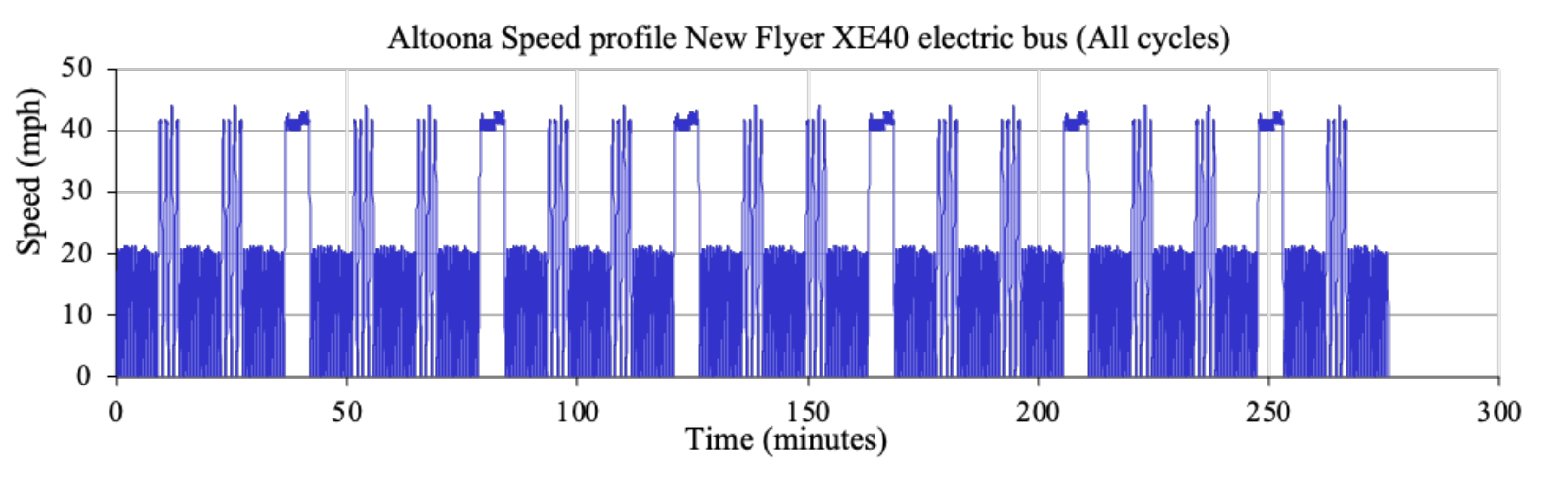
3.2.1. Validation Using Altoona Real-World Test Results

To validate our simulation model, we utilized the New Flyer XE40 Altoona test results [65]. The Altoona test is a real-world test for buses applied by Larson Transportation Institute’s Bus Research and Testing Center in Altoona, Pennsylvania. It is being used to test buses based on their performance, reliability, and fuel economy to provide a holistic assessment of bus performance [65].
The Altoona test, for the New Flyer XE40 BEB, utilized three driving cycles in the test procedures, including (a) the arterial (ART) cycle, with a length of 3.073 miles that represents the high capacity urban road with speed limits between 30 mph and 50 mph; (b) the central business district (CBD) cycle with a distance of 3.073 miles, which includes 14 repetitions of a basic cycle composed of idle, acceleration, and deceleration modes with an average speed of 20 mph; and (c) the commuter (COM) cycle, which represents urban cycles without any stops during the trip with an average speed of 40 mph [65]. We have extracted and used the three drive cycles (Appendix A) to validate the simulation model, which resulted in estimated energy consumption within ±3.81% (0.0381 kWh/km) accuracy (Figure 5). This is consistent with the results of [57]. More specifically, the differences in energy consumption between the Altoona test and our simulation model are 0.043 kWh/km (3%) in the ART cycle, 0.034 kWh/km (3.16%) in the CBD cycle, and 0.049 kWh/km (5.28%) in the COM cycle.

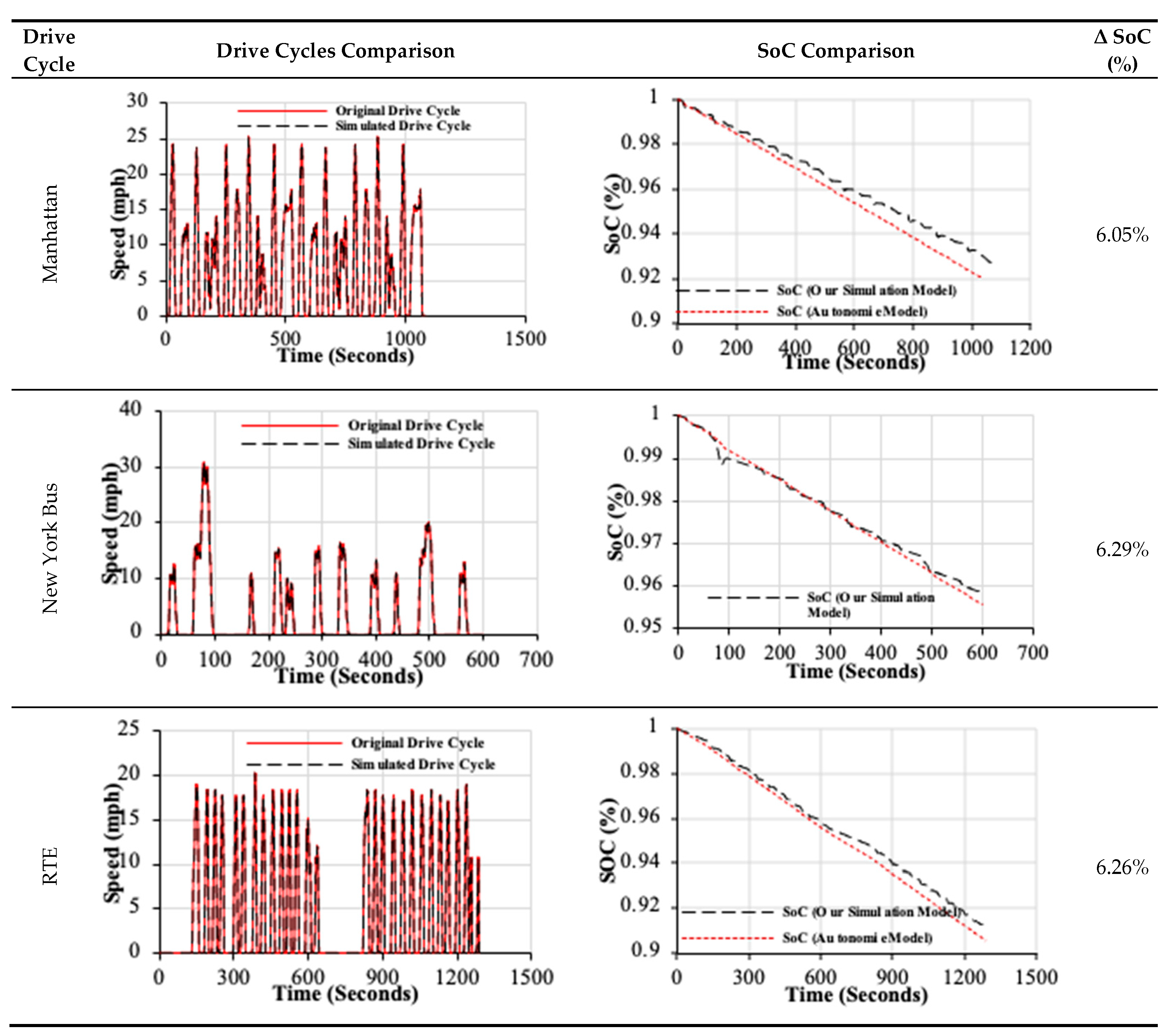
3.2.2. Validation Using Autonomie Software

Although the model validation through real-world Altoona test data provides a robust method to validate the model, some might argue that additional validation is required to cover the wide range of parameters used in the present study.
Therefore, we followed the approach utilized by Gao [38] and validated our model using Autonomie software. The Nova Bus model in Autonomie was reconfigured to include the powertrain parameters of the New Flyer XE40 BEB (Table 3). This reconfigured model was tested across three bus cycles; Manhattan, New York, and RTE. The Autonomie-predicted energy consumption is compared with our developed Simulink model across the same three cycles. The Autonomie validation process indicates only 6% error (simulated SoC minus Autonomie SoC), as depicted in Appendix B.

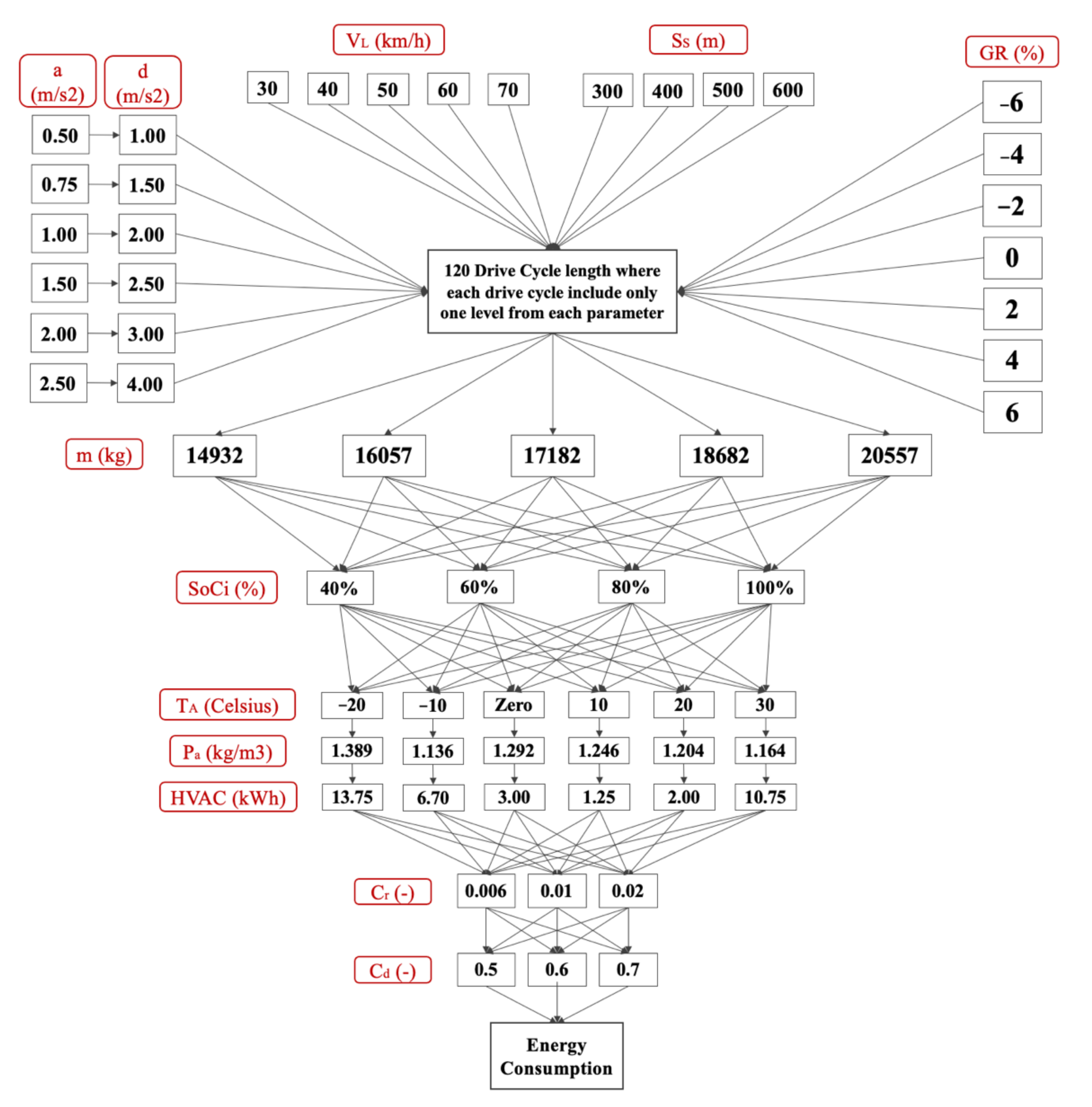
3.3. Full-Factorial Experiment Design

We designed a full-factorial experiment (i.e., all possible combinations) to generate scenarios for BEB operation and study the impacts of all parameters on BEB’s energy consumption. The experimental design included vehicular, operational, topological, and external parameters on different drive cycles. Although some might argue that the developed scenarios might reflect extreme conditions, their inclusion is fundamental for model development.
The parameters, and their levels, are defined based on the literature, as detailed in Table 4. We also collected field data and speed profiles for eight different bus routes with different terrains (using a high-definition GPS device) to ensure the diversity of the parameters such as road grade, speed limit, and spacing between stops. Since bus routes are inherently a mix of positive and negative gradients, it would not be accurate to model the effect of average grade on energy consumption. Therefore, we divided the eight-speed profiles into 120 drive cycles (i.e., segments) to accommodate the impact of parameters such as road gradient, average speed, acceleration rates, and deceleration rates on the energy consumption. Therefore, we obtained a constant road gradient for each drive cycle, following the assumptions of [20,66] to overcome the uncertainties in using the average road gradient.
Regarding vehicular and external parameters, we include four levels for the initial state of charge (40% till 100%, with 20% intervals). The total mass of the bus is calculated based on the curb weight and the number of passengers. The number of passengers is divided into five levels, where the minimum is zero passengers, while the maximum onboard capacity is 75 passengers. An average passenger weight (75 kg) is considered [51]. The HVAC power is estimated based on the ambient temperature following the model developed by [39] and modified by [29]. The ambient temperature (six levels) used to estimate the HVAC power has been considered to be between −20 °C and 30 °C based on the historical Canadian weather dataset [67]. The rolling resistance coefficient is considered based on the literature (three levels ranging from 0.006 to 0.02) [29,34,36].
Operational and topological parameters include the minimum and maximum rates for acceleration and deceleration, selected based on the literature and field observation, and represent both average and aggressive driving behaviours [34,36,68]. The rates varied between 0.50 m/s2 and 2.5 m/s2 for acceleration and 1 m/s2 to 4 m/s2 for deceleration, while the average speed is derived from the driving cycles. Furthermore, we used seven constant gradients levels ranging from −6% to 6%.
A total of 907,199 scenarios have been generated from all the possible combinations of the levels of the utilized parameters, using the full-factorial experimental design. We coded a loop in MATLAB to calculate the energy consumption rates for all generated scenarios, as shown in Figure 6. In the estimation process, only one parameter was changed, while all other parameters were fixed.

3.4. Prediction Model

Based on the inputs of the model, new parameters have been defined. The new parameters include passenger loading, which represents the number of passengers during the trip. The road condition includes three levels—I, II, and III—based on the utilized rolling resistance coefficient and taking into consideration a constant bus tire pressure. Level I refers to a good dry road condition that includes the rolling resistance coefficients ≤0.006. Level II refers to a fair wet road condition that includes rolling resistance coefficients ≥0.01 and <0.02, while level III refers to a poor icy road condition (slush) that includes rolling resistance coefficients ≥0.02.
The driver’s aggressiveness is defined based on the acceleration and deceleration rates of the bus drivers and divided into three levels. These levels are based on coupling six acceleration values with six deceleration values, resulting in a total of six pairs, which are grouped into three different levels, as depicted in Figure 6. Level I represents the slow driving behaviour with acceleration rates from 0.25 m/s2 to 0.5 m/s2 and deceleration rates from 1 m/s2 and 1.5 m/s2; level II represents the normal driving behaviour with acceleration rates from 1 m/s2 to 1.5 m/s2 and deceleration rates from 2 m/s2 and 2.5 m/s2; level III represents the aggressive driving behaviour with acceleration rates from 2 m/s2 to 2.5 m/s2 and deceleration rates from 3 m/s2 and 4 m/s2. In addition, a stop density parameter has been calculated by dividing the number of stops by the cycle length.
A multiple linear regression analysis (MLR) was applied to develop a prediction model for predicting the energy consumption of the BEBs. Besides, it quantifies the relationship between several independent parameters and a dependent parameter by fitting a linear equation to the observed dataset that we generated using the full-factorial experiment.
Given that the aim is to predict BEB energy consumption from vehicular, operational, topological, and external parameters, we used energy consumption (EC) as the dependant parameter. The independent parameters included the road grade (GR), driver aggressiveness (DAgg.), road condition (RC), HVAC, passenger loading (PL), stop density (SD), average speed (Va), the initial state of charge (SoCi), and route length (L), as depicted in Equation (18). Our model is based on predicting the EC in transit operation; thus, it can predict the EC for micro trips.
E C = β 0 + β 1 G R + β 2 D A g g + β 3 R C + β 4 H V A C + β 5 P L + β 6 S D + β 7 V a + β 8 S o C i + β 9 L + ε
where:
GR is the road grade (%),
DAgg. is the driver aggressiveness (three levels),
RC is the road condition (three levels),
HVAC is the consumed energy due to heating, ventilation, and air conditioning (kW),
PL is the passenger loading (passengers),
SD is the stop density ratio along the route (stops/km),
Va is the average speed during the trip (km/h),
SoCi is the initial state of the battery charge (%),
L is the route length (m).
A set of analyses has been carried out to evaluate the appropriateness for the model specification, including linearity, normality, homoscedasticity, and the outliers as recommended by [69]. The results of these analyses confirm the model specification.

4. Results

4.1. Descriptive Statistics

The descriptive statistics listed in Table 5 show the statistical properties of the parameters utilized in the model. The resultant energy consumption rates ranged between −2.490 kWh/km and 6.119 kWh/km with a mean of 1.654 kWh/km. It should be noted that negative energy consumption values are attributed to scenarios that include a constant negative grade. As such, the energy harnessed from the regenerative brake is higher than the energy consumed by the bus. The average number of passengers is approximately 38 passengers, while the stop density ranged between 1.651 stops/km and 3.486 stops/km. The driver aggressiveness and the road condition have a mean of 2.0 and standard deviation of 0.816, since both are divided into three levels.
The skewness and kurtosis are computed to test the normality of the data. The skewness values between 0.5 and −0.5 show the normal distribution of the utilized parameters [70]. The skewness values closer to zero indicate that the distribution is approximately symmetric, as shown in Table 5. The positive skewness values for Va, PL, SD, and HVAC indicate that the distribution is highly skewed to the left. Kurtosis between 2.0 and −2.0 is considered acceptable [70].
The correlation coefficients (Table 6) show significant correlations between the EC and the independent parameters. The results also indicate the lack of significant correlation between the independent parameters, except for route length and stop density (−0.979). Therefore, we excluded the route length parameter from the analysis. This was further assessed using statistical measures of multicollinearity (reported in the Results section) [71].

4.2. BEB Energy Consumption Prediction Model

Linearity, normality, multicollinearity, and homoscedasticity were evaluated to verify the multivariate statistical assumptions. The linearity test confirmed the linear relationship between the dependent and independent parameters through a high coefficient of determination (R2) for all the proposed regression models. Normality was confirmed through the errors between observed and predicted values (i.e., residuals), where a mean of 1.34 × 10⁻¹² and a standard deviation of 1.00 were obtained. Moreover, the linearity and normality of the model are tested graphically, as shown in Figure 7.
For multicollinearity, the magnitude of the correlation coefficients was less than 0.50 (Table 6), the variance inflation factor (VIF) values varied between 1.0 and 1.67 (<5), and tolerance ranged between 0.6 and 1.0 (>0.2), as shown in Table 7. These measures confirm the absence of multicollinearity between the parameters [64]. Finally, the homoscedasticity results indicate that the variance of error terms is similar across the independent parameters, given the absence of a systematic pattern of errors in the distribution in Figure 8 (1% of the data) and in Appendix C (100% of the data).
The model goodness-of-fit is evaluated by inspecting the residuals, the coefficient of determination (R2) (Table 7), outliers (Mahalanobis distance), and chi-square tests. The selected model shows a superior relationship between the dependent and independent parameters with an R2 of 0.961. The proposed model explained 96.1% of the variance in energy consumption rates. The t-test values exceeded ±1.96, indicating a significant difference in the effect of the independent parameters on the EC. Furthermore, the root means square error (RMSE) indicates the absolute fit of the model’s predicted values to the observed dataset. The RMSE value of 0.3167 reflects an accurate model.
Several relationships between the independent parameters and the dependent parameter (EC) are depicted in Figure 9. For each 3D plot, we fixed some independent parameters (bold top legend) while the remaining parameters varied. That said, the figure depicts the significant change in the energy consumption rates (at the bivariate level) resulting from the change in vehicular, operational, topological, and external parameters.
The standardized coefficients (betas) are used to compare the impact of each independent parameter on the energy consumption. Accordingly, road grade has a substantial impact on the EC (Std. β = 0.945), followed by the initial state of charge (Std. β = 0.172), road condition (Std. β = 0.132), HVAC (Std. β = 0.105), passenger loading (Std. β = 0.078), driver aggressiveness (Std. β = 0.033), and stop density (Std. β = 0.050), while the average speed has the lowest weight in affecting the EC (Std. β = 0.030). The prediction model is expressed mathematically in Equation (19).
E C = 0.782 + 0.380 G R + 0.0124 S o C i + 0.260 R C + 0.036   H V A C + 0.005 P L + 0.065 D A g g . + 0.128 S D + 0.007 V a + ε
Put another way, the increase in the road grade by 1% increases the EC by 0.380 kWh/km, while an increase in the initial state of charge by 10% increases the EC by 0.124 kWh/km. The variation in the road condition and driver aggressiveness from a level to another level affects the EC rates by 0.260 kWh/km and 0.065 kWh/km, respectively. The utilization of the HVAC system, which is attributed to temperature, has a significant bearing on the EC, while each 10 km/h increase in the average speed increases the EC rates by 0.07 kWh/km. Similarly, each increase in the stop density by one stop per km increases the EC rates by 0.128 kWh/km. An increase in the number of passengers by 10 passengers increases the consumed energy by 0.05 kWh/km, while an increase in HVAC by 1 kW increases the energy consumption by 0.036 kWh/km.

5. Discussion and Practical Relevance

5.1. Discussion of the Results

The estimated coefficients resulting from the multiple regression model show the significance of vehicular, operational, topological, and external parameters on the BEB’s consumed energy. Comparing our findings to previous studies shows that our model produced more significant parameters, as shown in Figure 10. The figure shows the normalized relative weight (per study) associated with the significant parameters reported to impact energy consumption. It considers the absolute impact ratio of the parameters without considering the sign to compare the results from regression models and sensitivity analysis.
The findings show that the main parameter driving the variation in the EC rates is the road grade. Considering that no previous study has investigated the impact of the road grade on the EC in the BEB literature, we compared our results with those in the EV literature. In this respect, [20,48,72] reported that road grade has the highest impact on EC, and it increases almost linearly with increasing the absolute gradient.
The road condition and the initial state of the charge are the second and third most significant parameters, respectively. Both parameters have a positive relationship with the EC rates, consistent with [29]. In contrast, Qi [52] found a negative relationship between the EC and the initial state of charge for EVs. However, Qi [21] argued that the state of charge is not significant in predicting the EC, yet it has a marginal impact on EC. Moreover, Vepsäläinen [29] indicated that the relation between energy consumption and the state of charge (less than 85%) is a fuzzy relationship. At the same time, the state of charge of more than 85% causes a lower energy recovery and therefore results in higher total energy consumption, which is in line with our results. We claim that the main reason for the high positive impact of the initial state of charge (SoCi) on the EC in the BEBs context is because our model is based on predicting the EC in transit operation, which exhibits micro trips. This might be the reason for the level of significance associated with the initial state of charge, especially in situations where the micro trip features a negative grade coupled with a full batter (i.e., SoCi around 100%). As such, the recovered energy from the regenerative break is marginal.
Regarding HVAC, the relationship between the ambient temperature and the consumed power is identified to have a non-linear relationship according to [73] and the model developed by [39]. To overcome this problem, the relationship between the ambient temperature and the HVAC power should be linearized around a specific value, as recommended by [27,37]. Our model was capable of capturing the significant impact of HVAC on EC by using the HVAC power as an input in our prediction model instead of using the ambient temperature.
Driver aggressiveness has a slightly low bearing, yet significant, on EC. The authors of [27,37,45] found a positive linear relationship between the driver aggressiveness and the EC. They concluded that the impact of driver aggressiveness on the EC is lower than the impact of the road condition, which supports our findings. Similarly, the increase in passenger loading causes a slight increase in EC rates. Franca [33] reported similar findings for BEBs.
Stop density has a positive relationship with the EC, indicating that increasing the number of stops contributes to higher energy consumption rates, which is in line with the results of [37], who stated a high positive linear relationship between the stop density and the energy consumption of BEB.
Comparing our model to the regression models available in the literature, our model has a higher goodness-of-fit than the previous models estimated by [37,46] and includes more significant parameters in the same model. The impact of road grade as a topological parameter in estimating the energy consumption is more representative than using the elevation difference mentioned by [46]. This is because using the elevation difference between points results in ignoring the distance between these points.
Overall, our study spans to cover energy consumption rates for various possible operation scenarios. This, in turn, mimics the real-world operation of bus transit systems, where the values of the utilized parameters are continuously changing during the bus trips. However, it should be noted that some additional variables might impact the energy consumption of BEBs that are not included in the present study.

5.2. Practical Implications

We aimed to develop a prediction model for BEB energy consumption that incorporates vehicular, operational, topological, and external parameters. Although this aim is achieved, the developed model holds significant practical implications to inform transit planners and decision-makers on the electrification of transit systems. These are articulated across two dimensions: BEB route selection and practical relevance.
First, we developed several hypothetical scenarios to inform transit planners on the best, moderate, and worst transit operational profile that enhances BEB energy utilization. The scenario development is based only on parameters associated with transit operation and design. Therefore, these scenarios incorporate average speed, stop density, passenger loading, driver aggressiveness, HVAC, and the initial state of charge, while they share a constant rolling grade (0%) and road condition (dry) (Table 8).
The scenario analysis indicates the significant bearing of transit network characteristics on the energy consumption of BEBs, which ranges from 1.109 to 3.055 kWh/km. Therefore, and considering operational parameters only, we encourage transit planners to implement BEBs on routes that feature lower stop density (one to two stops/km), coupled with higher traffic level of service (i.e., LoS A and B). The aim is to reduce the frequency of buses coming to a complete stop during operation. This recommendation is to enhance the energy utilization of BEBs, but not to say that BEBs are not feasible in routes with higher stop densities.
On the other hand, electrifying routes with higher average speed and/or low passenger loads would not significantly increase energy savings. That said, we also recommend transit planners to pay attention to road grade as the most significant parameter impacting BEB energy consumption.
Second, and concerning practical relevance, the proposed model could be implemented to quickly and efficiently model a transit network’s energy consumption without the need for sophisticated and technically advanced simulation models. Each route could be divided into several segments with similar characteristics (e.g., speed, stop density, and passenger loading) used as inputs in the proposed prediction model to estimate BEBs energy consumption. This would be very beneficial while planning for the electrification of transit networks.

6. Conclusions

The accurate estimation of BEB energy consumption is a challenging task that requires laborious work of identifying the details of the BEB transit networks and how they affect the consumed energy. In this respect, the present study reveals the causal relationship between the transit network parameters, including vehicular, operational, topological, and external parameters and BEB’s energy consumption, using multiple linear regression analysis. Furthermore, the study presents a prediction model for BEB energy consumption to inform the optimal bus route design that intensifies the BEB energy efficiency.
A simulation model had been developed to predict the energy consumption rates using MATLAB Simulink. The developed model is validated using New Flyer XE40 Altoona test results. The validation process shows very promising results with ±5% accuracy, which confirms the validity of the developed simulation model with respect to the range of parameters tested in Altoona cycles.
Moreover, we generated BEB energy consumption data using a full-factorial experiment and based on real-world data collection (907,199 scenarios). A multiple linear regression model (MLR) was developed from the selected scenarios to predict the relationship between the independent vehicular, operational, topological, and external parameters and the dependent energy consumption parameter.
The results reveal a significant relationship between the BEB energy consumption and the independent parameters, including the road grade, the initial state of charge, road condition, HVAC, passenger loading, driver aggressiveness, average speed, and stop density. Besides, the estimated coefficients show that the main parameter driving the variation in the energy consumption rates is the road grade, while the stop density had a lower impact. The validity of the prediction model was verified using the goodness-of-fit, which shows that the prediction model explains about 96.1% of the variance in energy consumption. The prediction model was validated using a second dataset of 169,344, showing a very accurate EC prediction.
Furthermore, we developed five hypothetical scenarios to inform the optimal transit operation profile design that improves energy efficiency. We encourage transit planners to pay attention to the road grade while planning the bus routes electrification since it is the most significant parameter that affects the BEB’s energy consumption. Additionally, routes with lower stop density should be considered for transit electrification. Simultaneously, the average speed and passenger loading do not have a considerable bearing, but a significant one, on the consumed energy compared to other parameters.
Although our results are in line with previous studies related to BEBs and EVs energy consumption, our study has some limitations. First, the regenerative braking energy recovery is considered in the energy consumption estimation. Yet, we did not study the impact of operational parameters on the change of the regenerative braking energy recovery. Additionally, in our model, auxiliary power was used at a constant rate, which is sensitive to the operation conditions (e.g., boarding/dwelling). Therefore, we encourage future studies to accommodate these limitations.

Author Contributions

Conceptualization, M.M.; methodology, H.A. and M.M.; software, H.A.; validation, H.A.; formal analysis, H.A.; investigation, H.A.; resources, M.M.; data curation, H.A. and M.M.; writing—original draft preparation, H.A. and M.M.; writing—review and editing, M.M.; visualization, H.A.; supervision, M.M.; project administration, M.M.; funding acquisition, M.M. Both authors have read and agreed to the published version of the manuscript.

Funding

This research was funded by the Natural Sciences and Engineering Research Council of Canada (NSERC) Grant No: RGPIN-2018-05994.

Institutional Review Board Statement

Not applicable.

Informed Consent Statement

Not applicable.

Data Availability Statement

Not applicable.

Acknowledgments

The authors would like to that the editor and the reviewers for their constructive comments.

Conflicts of Interest

The authors declare no conflict of interest.

Appendix A. Altoona Speed Profile

Figure A1. Altoona’s combined speed profiles.
Energies 14 02824 g0a1

Appendix B. Autonomie-Based Validation of the Developed Simulink Model

Figure A2. Autonomie based energy consumption model validation.
Energies 14 02824 g0a2

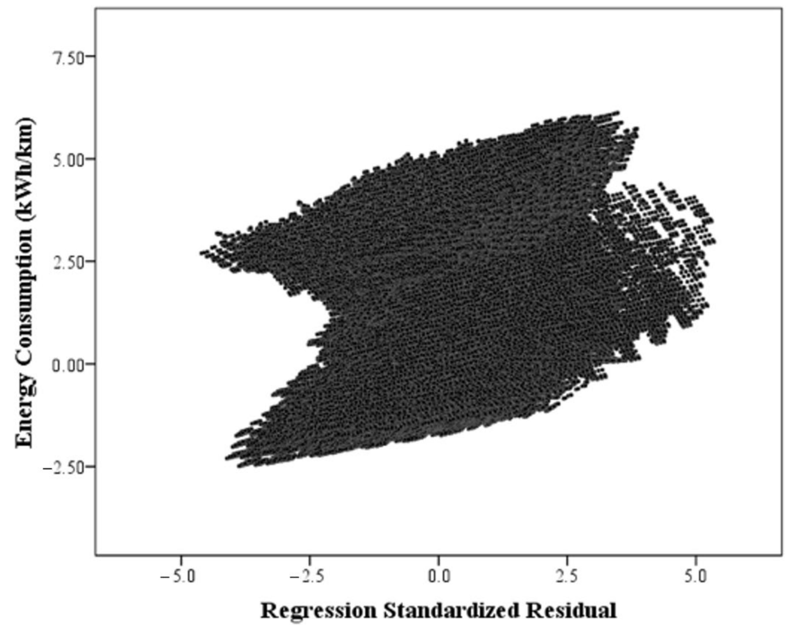
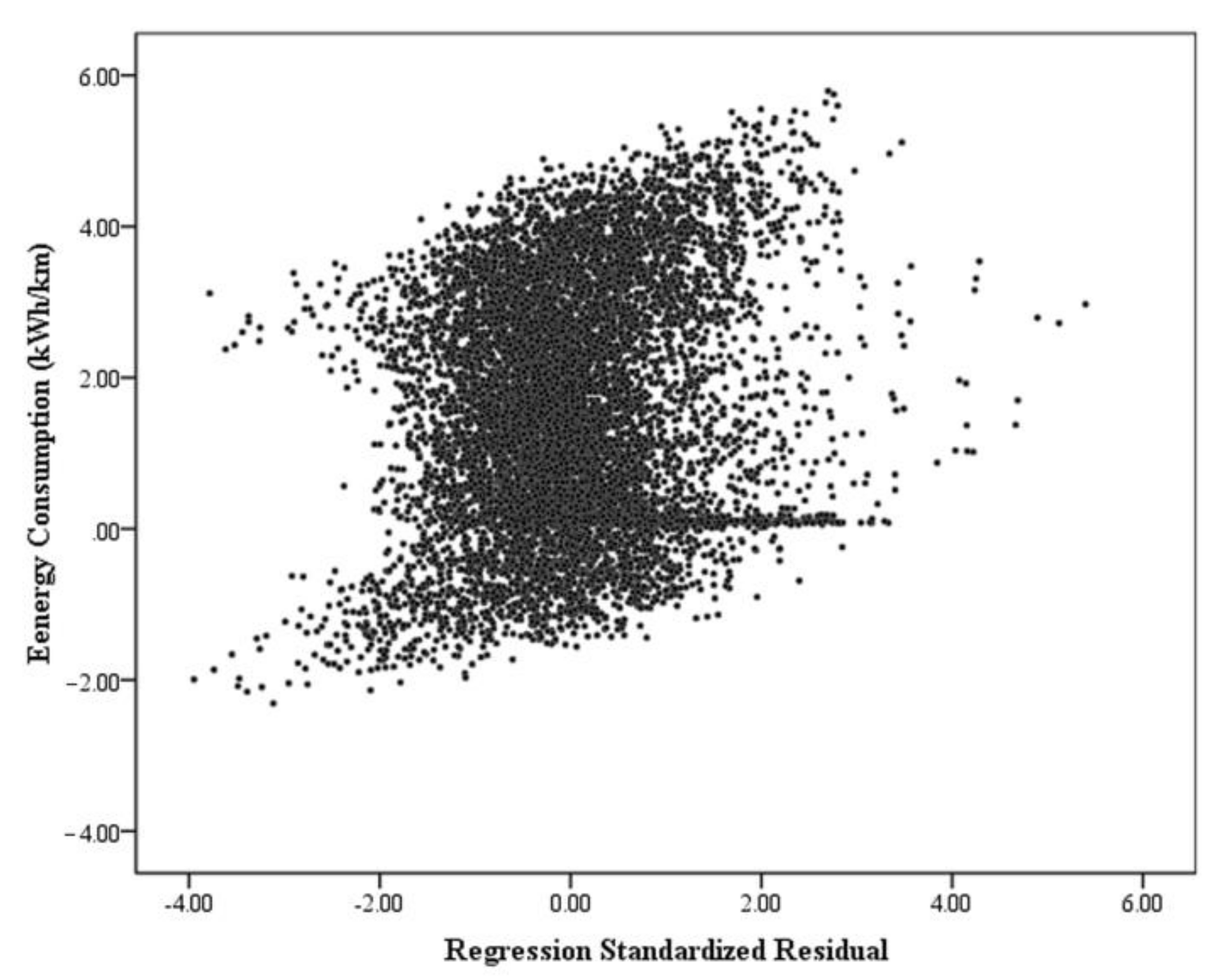
Appendix C. A Scatter Plot for the Regression Standardized Residuals (n = 907,199)

Figure A3. A scatter plot for the regression standardized residuals (n = 907,199)
Energies 14 02824 g0a3

References

  1. Perrotta, D.; Macedo, J.L.; Rossetti, R.J.; De Sousa, J.F.; Kokkinogenis, Z.; Ribeiro, B.; Afonso, J.L. Route Planning for Electric Buses: A Case Study in Oporto. Procedia Soc. Behav. Sci. 2014, 111, 1004–1014. [Google Scholar] [CrossRef] [Green Version]
  2. Markel, T.; Brooker, A.; Hendricks, T.; Johnson, V.; Kelly, K.; Kramer, B.; O’Keefe, M.; Sprik, S.; Wipke, K. ADVISOR: A systems analysis tool for advanced vehicle modeling. J. Power Sources 2002, 110, 255–266. [Google Scholar] [CrossRef]
  3. Ferguson, M.; Mohamed, M.; Maoh, H. On the Electrification of Canada’s Vehicular Fleets: National-scale analysis shows that mindsets matter. IEEE Electrif. Mag. 2019, 7, 55–65. [Google Scholar] [CrossRef]
  4. Mohamed, M.; Higgins, C.; Ferguson, M.; Kanaroglou, P. Identifying and characterizing potential electric vehicle adopters in Canada: A two-stage modelling approach. Transp. Policy 2016, 52, 100–112. [Google Scholar] [CrossRef]
  5. Kennedy, C. Key threshold for electricity emissions. Nat. Clim. Chang. 2015, 5, 179–181. [Google Scholar] [CrossRef]
  6. Mahmoud, M.; Garnett, R.; Ferguson, M.; Kanaroglou, P. Electric buses: A review of alternative powertrains. Renew. Sustain. Energy Rev. 2016, 62, 673–684. [Google Scholar] [CrossRef]
  7. Borén, S. Electric buses’ sustainability effects, noise, energy use, and costs. Int. J. Sustain. Transp. 2020, 14, 1–16. [Google Scholar] [CrossRef] [Green Version]
  8. Kühne, R. Electric buses—An energy efficient urban transportation means. Energy 2010, 35, 4510–4513. [Google Scholar] [CrossRef]
  9. Mohamed, M.; Farag, H.; El-Taweel, N.; Ferguson, M. Simulation of electric buses on a full transit network: Operational feasibility and grid impact analysis. Electr. Power Syst. Res. 2017, 142, 163–175. [Google Scholar] [CrossRef]
  10. Quarles, N.; Kockelman, K.M.; Mohamed, M. Costs and Benefits of Electrifying and Automating Bus Transit Fleets. Sustainability 2020, 12, 3977. [Google Scholar] [CrossRef]
  11. Wellik, T.K.; Griffin, J.R.; Kockelman, K.M.; Mohamed, M. Utility-transit nexus: Leveraging intelligently charged electrified transit to support a renewable energy grid. Renew. Sustain. Energy Rev. 2021, 139. [Google Scholar] [CrossRef]
  12. Mohamed, M.; Ferguson, M.; Kanaroglou, P. What hinders adoption of the electric bus in Canadian transit? Perspectives of transit providers. Transp. Res. Part D Transp. Environ. 2018, 64, 134–149. [Google Scholar] [CrossRef]
  13. Chen, F.; Fernandes, T.; Roche, M.Y.; Carvalho, M.D.G. Investigation of challenges to the utilization of fuel cell buses in the EU vs transition economies. Renew. Sustain. Energy Rev. 2007, 11, 357–364. [Google Scholar] [CrossRef]
  14. El-Taweel, N.A.; Farag, H.E.Z.; Mohamed, M. Integrated Utility-Transit Model for Optimal Configuration of Battery Electric Bus Systems. IEEE Syst. J. 2020, 14, 738–748. [Google Scholar] [CrossRef]
  15. Liu, Z.; Song, Z.; He, Y. Economic Analysis of On-Route Fast Charging for Battery Electric Buses: Case Study in Utah. Transp. Res. Rec. J. Transp. Res. Board 2019, 2673, 119–130. [Google Scholar] [CrossRef]
  16. Abdelaty, H.; Elsayed, M.; Mohamed, M. Assessing the feasibility of energy storage system for electric bus transit planning. In Proceedings of the 55th Annual Canadian Transportation Research Forum, Montreal, QC, Canada, 24–27 May 2020; pp. 1–21. [Google Scholar]
  17. El-Taweel, N.A.; Mohamed, M.; Farag, H.E. Optimal design of charging stations for electrified transit networks. In Proceedings of the 2017 IEEE Transportation Electrification Conference and Expo (ITEC), Chicago, IL, USA, 22–24 June 2017; pp. 786–791. [Google Scholar]
  18. He, Y.; Song, Z.; Liu, Z. Fast-charging station deployment for battery electric bus systems considering electricity demand charges. Sustain. Cities Soc. 2019, 48, 101530. [Google Scholar] [CrossRef] [Green Version]
  19. Rupp, M.; Rieke, C.; Handschuh, N.; Kuperjans, I. Economic and ecological optimization of electric bus charging considering variable electricity prices and CO2eq intensities. Transp. Res. Part D Transp. Environ. 2020, 81, 102293. [Google Scholar] [CrossRef]
  20. Liu, K.; Yamamoto, T.; Morikawa, T. Impact of road gradient on energy consumption of electric vehicles. Transp. Res. Part D Transp. Environ. 2017, 54, 74–81. [Google Scholar] [CrossRef]
  21. Qi, X.; Wu, G.; Boriboonsomsin, K.; Barth, M.J. Data-driven decomposition analysis and estimation of link-level electric vehicle energy consumption under real-world traffic conditions. Transp. Res. Part D Transp. Environ. 2018, 64, 36–52. [Google Scholar] [CrossRef] [Green Version]
  22. Teoh, L.E.; Khoo, H.L.; Goh, S.Y.; Chong, L.M. Scenario-based electric bus operation: A case study of Putrajaya, Malaysia. Int. J. Transp. Sci. Technol. 2018, 7, 10–25. [Google Scholar] [CrossRef]
  23. Vepsäläinen, J.; Kivekäs, K.; Otto, K.; Lajunen, A.; Tammi, K. Development and validation of energy demand uncertainty model for electric city buses. Transp. Res. Part D Transp. Environ. 2018, 63, 347–361. [Google Scholar] [CrossRef]
  24. Wang, J.; Kang, L.; Liu, Y. Optimal scheduling for electric bus fleets based on dynamic programming approach by considering battery capacity fade. Renew. Sustain. Energy Rev. 2020, 130, 109978. [Google Scholar] [CrossRef]
  25. Zhou, B.; Wu, Y.; Zhou, B.; Wang, R.; Ke, W.; Zhang, S.; Hao, J. Real-world performance of battery electric buses and their life-cycle benefits with respect to energy consumption and carbon dioxide emissions. Energy 2016, 96, 603–613. [Google Scholar] [CrossRef]
  26. Basso, R.; Kulcsár, B.; Egardt, B.; Lindroth, P.; Sanchez-Diaz, I. Energy consumption estimation integrated into the Electric Vehicle Routing Problem. Transp. Res. Part D Transp. Environ. 2019, 69, 141–167. [Google Scholar] [CrossRef]
  27. De Cauwer, C.; Van Mierlo, J.; Coosemans, T. Energy Consumption Prediction for Electric Vehicles Based on Real-World Data. Energies 2015, 8, 8573–8593. [Google Scholar] [CrossRef]
  28. Kivekäs, K.; Lajunen, A.; Vepsäläinen, J.; Tammi, K. City Bus Powertrain Comparison: Driving Cycle Variation and Passenger Load Sensitivity Analysis. Energies 2018, 11, 1755. [Google Scholar] [CrossRef] [Green Version]
  29. Vepsäläinen, J.; Otto, K.; Lajunen, A.; Tammi, K. Computationally efficient model for energy demand prediction of electric city bus in varying operating conditions. Energy 2019, 169, 433–443. [Google Scholar] [CrossRef]
  30. Abdelaty, H.; Mohamed, M. Uncertainty in Electric Bus Energy Consumption: The Impacts of Grade and Driving Behaviour. In Proceedings of the 55th Annual Canadian Transportation Research Forum, Montreal, QC, Canada, 24–27 May 2020. [Google Scholar]
  31. Abdelaty, H.; Al-Obaidi, A.; Mohamed, M.; Farag, H.E.Z. Machine Learning Prediction Models for Battery-Electric Bus Energy Consumption in Transit. Transp. Res. Part D Transp. Environ. 2021. [Google Scholar]
  32. Kunith, A.; Mendelevitch, R.; Goehlich, D. Electrification of a city bus network—An optimization model for cost-effective placing of charging infrastructure and battery sizing of fast-charging electric bus systems. Int. J. Sustain. Transp. 2017, 11, 707–720. [Google Scholar] [CrossRef] [Green Version]
  33. Franca, A. Electricity Consumption and Battery Lifespan Estimation for Transit Electric Buses: Drivetrain Simulations and Electrochemical Modelling; University of Victoria: Victoria, BC, Canada, 2015. [Google Scholar]
  34. Gallet, M.; Massier, T.; Hamacher, T. Estimation of the energy demand of electric buses based on real-world data for large-scale public transport networks. Appl. Energy 2018, 230, 344–356. [Google Scholar] [CrossRef]
  35. Lajunen, A. Energy consumption and cost-benefit analysis of hybrid and electric city buses. Transp. Res. Part C Emerg. Technol. 2014, 38, 1–15. [Google Scholar] [CrossRef]
  36. Lajunen, A. Lifecycle costs and charging requirements of electric buses with different charging methods. J. Cleaner Prod. 2018, 172, 56–67. [Google Scholar] [CrossRef]
  37. Vepsäläinen, J.; Ritari, A.; Lajunen, A.; Kivekäs, K.; Tammi, K. Energy Uncertainty Analysis of Electric Buses. Energies 2018, 11, 3267. [Google Scholar] [CrossRef] [Green Version]
  38. Gao, Z.; Lin, Z.; LaClair, T.J.; Liu, C.; Li, J.-M.; Birky, A.K.; Ward, J. Battery capacity and recharging needs for electric buses in city transit service. Energy 2017, 122, 588–600. [Google Scholar] [CrossRef] [Green Version]
  39. Lajunen, A.; Tammi, K. Energy consumption and carbon dioxide emission analysis for electric city buses. In Proceedings of the 29th World Electric Vehicle Symposium and Exhibition (EVS29), Montreal, QC, Canada, 19–22 June 2016. [Google Scholar]
  40. Diaz Alvarez, A.; Serradilla Garcia, F.; Naranjo, J.E.; Anaya, J.J.; Jimenez, F. Modeling the Driving Behavior of Electric Vehicles Using Smartphones and Neural Networks. IEEE Intell. Transp. Syst. Mag. 2014, 6, 44–53. [Google Scholar] [CrossRef]
  41. Basma, H.; Mansour, C.; Nemer, M.; Stabat, P.; Haddad, M. Sensitivity analysis of bus line electrification at different operating conditions. In Proceedings of the 8th Transport Research Arena TRA, Helsinki, Finland, 27–30 April 2020; pp. 1–10. [Google Scholar]
  42. Bajtelsmit, V. Risk Analysis and the Optimal Capital Budget; Lecture notes; University of Missouri: St. Louis, MO, USA, 1997. [Google Scholar]
  43. Christopher Frey, H.; Patil, S.R. Identification and Review of Sensitivity Analysis Methods. Risk Anal. 2002, 22, 553–578. [Google Scholar] [CrossRef]
  44. Yuan, X.; Zhang, C.; Hong, G.; Huang, X.; Li, L. Method for evaluating the real-world driving energy consumptions of electric vehicles. Energy 2017, 141, 1955–1968. [Google Scholar] [CrossRef]
  45. De Cauwer, C.; Verbeke, W.; Coosemans, T.; Faid, S.; Van Mierlo, J. A Data-Driven Method for Energy Consumption Prediction and Energy-Efficient Routing of Electric Vehicles in Real-World Conditions. Energies 2017, 10, 608. [Google Scholar] [CrossRef] [Green Version]
  46. Pamula, T.; Pamula, W. Estimation of the Energy Consumption of Battery Electric Buses for Public Transport Networks Using Real-World Data and Deep Learning. Energies 2020, 13, 2340. [Google Scholar] [CrossRef]
  47. Galvin, R. Energy consumption effects of speed and acceleration in electric vehicles: Laboratory case studies and implications for drivers and policymakers. Transp. Res. Part D Transp. Environ. 2017, 53, 234–248. [Google Scholar] [CrossRef]
  48. Wang, J.-B.; Liu, K.; Yamamoto, T.; Morikawa, T. Improving Estimation Accuracy for Electric Vehicle Energy Consumption Considering the Effects of Ambient Temperature. Energy Procedia 2017, 105, 2904–2909. [Google Scholar] [CrossRef]
  49. Neaimeh, M.; Hill, G.A.; Hübner, Y.; Blythe, P.T. Routing systems to extend the driving range of electric vehicles. IET Intell. Transp. Syst. 2013, 7, 327–336. [Google Scholar] [CrossRef] [Green Version]
  50. Kivekäs, K.; Vepsäläinen, J.; Tammi, K.; Anttila, J. Influence of Driving Cycle Uncertainty on Electric City Bus Energy Consumption. In Proceedings of the 2017 IEEE Vehicle Power and Propulsion Conference (VPPC), Belfort, France, 11–14 December 2017; pp. 1–5. [Google Scholar]
  51. Lajunen, A.; Kivekaes, K.; Baldi, F.; Vepsaelaeinen, J.; Tammi, K. Different Approaches to Improve Energy Consumption of Battery Electric Buses. In Proceedings of the 2018 IEEE Vehicle Power and Propulsion Conference (VPPC), Chicago, IL, USA, 27–30 August 2018; pp. 1–6. [Google Scholar]
  52. Qi, Z.; Yang, J.; Jia, R.; Wang, F. Investigating Real-World Energy Consumption of Electric Vehicles: A Case Study of Shanghai. Procedia Comput. Sci. 2018, 131, 367–376. [Google Scholar] [CrossRef]
  53. Liu, K.; Wang, J.; Yamamoto, T.; Morikawa, T. Exploring the interactive effects of ambient temperature and vehicle auxiliary loads on electric vehicle energy consumption. Appl. Energy 2018, 227, 324–331. [Google Scholar] [CrossRef]
  54. Zhang, R.; Yao, E. Electric vehicles’ energy consumption estimation with real driving condition data. Transp. Res. Part D Transp. Environ. 2015, 41, 177–187. [Google Scholar] [CrossRef]
  55. Badin, F.; Le Berr, F.; Briki, H.; Dabadie, J.-C.; Petit, M.; Magand, S.; Condemine, E. Evaluation of EVs energy consumption influencing factors, driving conditions, auxiliaries use, driver’s aggressiveness. In Proceedings of the 2013 World Electric Vehicle Symposium and Exhibition (EVS27), Barcelona, Spain, 17–20 November 2013; pp. 1–12. [Google Scholar]
  56. Hahn, B.; Valentine, D. SIMULINK® Toolbox. In Essential MATLAB for Engineers and Scientists; Academic Press: Cambridge, MA, USA, 2019. [Google Scholar]
  57. De Filippo, G.; Marano, V.; Sioshansi, R. Simulation of an electric transportation system at The Ohio State University. Appl. Energy 2014, 113, 1686–1691. [Google Scholar] [CrossRef]
  58. Rodríguez Pardo, M. Uncertainty in Electric Bus Mass and Its Influence in Energy Consumption; Aalto University: Espoo, Finland, 2017. [Google Scholar]
  59. Beckers, C.J.J.; Besselink, I.J.M.; Frints, J.J.M.; Nijmeijer, H. Energy consumption prediction for electric city buses. In Proceedings of the 13th ITS European Congres, Eindhoven, The Netherlands, 3–6 June 2019. [Google Scholar]
  60. Reimpell, J.; Stoll, H.; Betzler, J.W. The Automotive Chassis: Engineering Principles; Butterworth-Heinemann: Woburn, MA, USA, 2001. [Google Scholar]
  61. Hogan, C.M.; Latshaw, G.L. The relationship between highway planning and urban noise. In Proceedings of the ASCE Urban Transportation Division Environment Impact Specialty Conference, Chicago, IL, USA, 21–23 May 1973; pp. 109–126. [Google Scholar]
  62. Pelkmans, L.; De Keukeleere, D.; Bruneel, H.; Lenaers, G. Influence of Vehicle Test Cycle Characteristics on Fuel Consumption and Emissions of City Buses. SAE Trans. 2001, 110, 1388–1398. [Google Scholar]
  63. NewFlyer-XE40. Xcelsior Charge Technical Summary—40′ Electric Bus; New Flyer: Anniston, AL, USA, 2017. [Google Scholar]
  64. James, G.M.; Hastie, T.; Witten, D.; Tibshirani, R. An Introduction to Statistical Learning: With Applications in R; Springer: New York, NY, USA, 2013. [Google Scholar]
  65. Altoona. Federal Transit Bus Test, Manufacturer: New Flyer, Model: XE40; Pennsylvania Transportation Institute: Pennsylvania, PA, USA, 2015. [Google Scholar]
  66. Sagaama, I.; Kchiche, A.; Trojet, W.; Kamoun, F. Impact of Road Gradient on Electric Vehicle Energy Consumption in Real-World Driving; Barolli, L., Amato, F., Moscato, F., Enokido, T., Takizawa, M., Eds.; Springer International Publishing: Cham, Switzerland, 2020; pp. 393–404. [Google Scholar]
  67. Government of Canada. Canada Daily Data Report, Environment and Natural Resources. Weather, Climate and Hazard; Government of Canada: Toronto, ON, Canada, 2019.
  68. Kontou, A.; Miles, J. Electric Buses: Lessons to be Learnt from the Milton Keynes Demonstration Project. Procedia Eng. 2015, 118, 1137–1144. [Google Scholar] [CrossRef] [Green Version]
  69. Joseph, F.; Hair, J.; Black, W.C.; Babin, B.J.; Anderson, R.E. Multivariate Data Analysis, 7th ed.; Pearson Education Limited: Harlow, UK, 2009. [Google Scholar]
  70. George, D.; Mallery, P. SPSS for Windows Step by Step: A Simple Guide and Reference; Prentice Hall Press: Hoboken, NJ, USA, 2010. [Google Scholar]
  71. Hair, J.; Black, W.; Babin, B.; Anderson, R. Multivariate Data Analysis; Pearson Prentice Hall: Upper Saddle River, NJ, USA, 2010. [Google Scholar]
  72. Liu, K.; Wang, J.; Yamamoto, T.; Morikawa, T. Modelling the multilevel structure and mixed effects of the factors influencing the energy consumption of electric vehicles. Appl. Energy 2016, 183, 1351–1360. [Google Scholar] [CrossRef]
  73. Melaina, M.; Bush, B.; Eichman, J.; Wood, E.; Stright, D.; Krishnan, V.; Keyser, D.; Mai, T.; McLaren, J. National Economic Value Assessment of Plug-In Electric Vehicles; National Renewable Energy Laboratory (NREL): Golden, CO, USA, 2016.
Figure 1. Parameters impacting the energy consumption of battery-electric buses.
Energies 14 02824 g001
Figure 2. A simple flow chart of the four-step methodology.
Energies 14 02824 g002
Figure 3. MATLAB Simulink model configuration for BEB powertrain.
Energies 14 02824 g003
Figure 4. The longitudinal forces acting on the bus movements.
Energies 14 02824 g004
Figure 5. Energy consumption in the Altoona test compared to the developed simulation model.
Energies 14 02824 g005
Figure 6. Full-factorial experimental design parameters (907,199 scenarios).
Energies 14 02824 g006
Figure 7. The distribution of the regression standardized residuals.
Energies 14 02824 g007
Figure 8. A scatter plot for the regression standardized residuals (n = 9071 1% of the data).
Energies 14 02824 g008
Figure 9. 3D plots for the relationships between EC and the independent parameters.
Energies 14 02824 g009aEnergies 14 02824 g009bEnergies 14 02824 g009c
Figure 10. The relative weight (normalized per study) of significant parameters impacting electric powertrains energy consumption.
Energies 14 02824 g010
Table 1. Parameters affecting the energy consumption of BEB in the literature.
Vehicular ParametersOperational ParametersTopological ParametersExternal Parameters
MassFrontal AreaDrag CoefficientRolling ResistanceBattery TemperatureInitial State of ChargeNumber of StopsSpacing between StopsAverage SpeedAcceleration RateDeceleration RateRoute LengthRoad GradeAmbient TemperatureAir
Density
Auxiliary PowerHVAC
m‰
(ton)
A F
(m2)
C d C r T B
(°C)
S o C i
(%)
S N S s
(m)
V a
(Km/h)
a‰
(m/s2)
d‰
(m/s2)
L
(Km)
GR‰
(%)
T A
(°C)
P a
(Kg/m3)
A u x
(kW)
HVAC
(kW)
Gallet [34] 10.00
12.50
15.00
17.50
18.50
8.30
10.35
0.60
0.70
0.80
0.006
0.008
0.010
--5-11.50
18.90
19.10
20.00
36.60
0.70
1.00
2.00
1.00
1.50
2.50
0.236
0.384
0.600
0.662
0.948
--1.188
10
12
15
-
Vepsäläinen [29] 8.50
to
15.00
--0.006
to
0.020
15
to
30
100
to
50
-------−30 to 35-2 to 72 to 25
Vepsäläinen [23] 12.40
14.80
6.200.600.010208918-24.201.67 (max)2.57
(max)
10.100-51.27--
Kivekäs [50] 10.35
12.35
15.00
6.200.500.008--25-20.580.55
(avg.)
0.51
(avg.)
10.422 ---1.50-
Lajunen [35] 8.50 to
15.00
6.200.700.008----20.380.54
(avg.)
0.50
(avg.)
------
Lajunen [51] 12.70
14.65
--0.008
0.012
----10.9 to 41.20.15 to
0.33
-3.3 to 42.40.00 to
+9.69
--6.00
9.00
-
Franca [33] 16.928.900.660.008----20.231.50
1.30 (avg.)
2.50
2.70 (max)
3.22---2.50-
Gao [38] 10.44
15.63
8.500.790.0098----5.75
11.00
13.42
19.85
3.00
4.06
4.60
6.10
4.30
4.50
5.13
5.60
0.98
6.65
6.86
10.53
---3.75-
Lajunen [36] 10.006.200.600.010---99
175
344
384
714
1250
5.90
11.00
19.80
22.50
31.50
41.20
1.40
1.80
2.10
2.40
2.80
-
1.90
2.10
2.30
2.50
3.60
-
1.00
3.30
10.30
10.50
10.90
28.60
-----
Kunith [32] 12.50
17.50
8.28
10.35
0.660.008---------−15 to 301.292.57 to 17.06-
Minimum8.506.200.500.00615505995.750.150.500.2360.00−301.181.502.00
Maximum20.0010.350.800.0203010025125041.206.105.6042.409.69351.2917.0625.00
Mean,
(St. d)
14.260 (3.35)7.948 (1.674)0.661
(0.0920)
0.0094 (0.0035)21.667
(7.638)
79.667 (26.274)16
(10.149)
494.333 (427.15)20.262
(10.232)
2.000
(1.563)
−2.688
(1.504)
8.095
(10.486)
4.845
(6.852)
5
(28.062)
1.247
(0.059)
7.414
(5.072)
13.50
(16.26)
Table 2. A concise list of regression models used to predict energy consumption for BEBs and EV.
Model ParametersModel TypeMode
Pamula and Pamula [46]Spacing between Stops, Travel Time, Elevation Differences, Weather ConditionLinear RegressionBus
Teoh [22]Route Length, Number of PassengersLinear RegressionBus
Vepsäläinen [37] Idle Time, Driver Aggressiveness, Average speed, Stops per Km, Ambient Temperature, initial State of ChargeLinear RegressionBus
Qi [52]Initial State of Charge, Average Temperature, Route Length, Average SpeedLinear RegressionVehicle
Liu [53] HVAC, Average speed, Route Length, Ambient Temperature, Road Grade (−9% to 9%)Ordinary Least Squares Regression
Multilevel Mixed Effects Linear Regression.
Vehicle
Wang [48] Linear Regression
Multilevel Linear Regression
Vehicle
Liu [20] Route Length, Average Speed, A/C and Heater Usage Ratio, Road Grade (−9% to 11%)Linear Regression
Three-Level Mixed Effects Models
Vehicle
De Cauwer [45] Rolling Resistance, Aerodynamic Drag, Temperature, Auxiliary Power, Route Length, Travel Time, Acceleration/Deceleration Rates, Vehicle and Wind Speed, ElevationLinear RegressionVehicle
Yuan [44] Road Grade, Acceleration/Deceleration Rates, Air Conditioning, Rolling Resistance, Aerodynamic Drag, Ambient TemperatureLinear RegressionVehicle
Galvin [47] Acceleration/Deceleration Rates, Maximum Speed, Route Length, Average Speed, Travel TimeLinear RegressionVehicle
De Cauwer [27] Rolling resistance, Aerodynamic Drag, Auxiliary Power, Elevation, Acceleration/Deceleration RatesLinear RegressionVehicle
Zhang and Yao [54] Instantaneous Speed, Acceleration Rates, State of ChargeLinear RegressionVehicle
Neaimeh [49] Road Grade (−6% to 6%), Average SpeedLinear RegressionVehicle
Badin [55]Average Speed, Acceleration Rates, Stop Duration, Auxiliary Power, Regenerative BrakeSimulation Model resulted in a Non-linear effectVehicle
Table 3. Base model parameters for BEB energy consumption simulation.
ParameterValue
Bus SpecificationBattery Initial State of Charge (%)100
Max. Torque (N.m.)2500
Battery Capacity (kWh)200
Frontal area (m2)8.32
Dynamic Radius of the Tires (m)0.5
Gear Ratio4.66
Curb Weight (kg)14,860
Recharge Efficiency0.978
Round Trip Efficiency0.971
Motor Efficiency0.916
Discharge Efficiency0.992
Base-model SpecificationDrag Coefficient0.6
Rolling Resistance0.01
Air Density (kg/m3)1.27
Ambient Temperature (o)20
HVAC (kW)0
Auxiliary Power (kW)*0
* As Auxiliary power (AUX) is not reported in Altoona Test, a value of Zero was used in the base simulation model.
Table 4. List of input parameters used in full-factorial experiment design.
Parameter—Unit ParameterLevelsMin.Max.MeanStandard Deviation
Initial state of charge (SoCi)—%Vehicular and
External
44010070.0022.36
Mass (m)—Kg514,93220,55717,4821975.792
HVAC—kW61.2513.756.244.66
Rolling resistance (Cr)—Unitless30.0060.020.01200.0059
Road grade (GR)—%Operational
and
Topological
7−6+60.004.00
Average speed (Va)—Km/h12019.9949.9531.966.81
Maximum speed (Vm)—Km/h12031.6072.9151.6713.66
Acceleration rates (a)—m/s260.52.51.380.70
Deceleration rates (d)—m/s26142.330.99
Spacing between stops (SS)—m4300600450.00111.80
Cycle Length (L)—m120860.541817.0001347.89332.35
Total number of unique scenarios907,199
Table 5. Descriptive statistics of the dataset (n = 907,199).
ParameterMinMaxMeanStandard ErrorSt.DSkewnessSkewness
Std. Error
KurtosisKurtosis Std. Error
EC—(kWh/km)−2.4906.1191.6540.0021.6090.0550.003−0.8900.005
g—(%)−6.0006.0000.0000.0424.0000.0000.003−1.2500.005
SoCi—(%)40.000100.00070.0000.00023522.3610.0000.003−1.3600.005
RC—(level)1.0003.0002.0000.0010.8160.0000.003−1.5000.005
PL—(passenger)0.00075.00034.0000.02826.3440.2930.003−1.1900.005
DAgg.—(level)1.0003.0002.0000.0010.8160.0000.003−1.5000.005
Va—(km/h)19.98649.95431.9640.0076.8070.4590.003−0.5590.005
SD—(Stop/km)1.6513.4862.3770.00060.6250.4770.003−1.1940.005
HVAC—(kW)1.25013.7506.2420.0054.6610.4610.003−1.3590.005
L—(m)860.5361817.0001347.8910.350333.3540.0060.003−1.3530.005
Table 6. The correlation matrix for the utilized parameters.
ECgSoCiRCPLDAgg.VaSDHVACL
EC1.000
GR0.945 **1.000
SoCi0.172 **0.0001.000
RC0.132 **0.0000.0001.000
PL0.078 **0.0000.0000.0001.000
DAgg.0.049 **0.0000.0000.0000.0001.000
Va0.027 **0.0000.0000.0000.0000.491 **1.000
SD0.039 **0.0000.0000.0000.0000.025 **−0.388 *1.000
HVAC0.105 **0.0000.0000.0000.0000.0000.0000.0001.000
L−0.037 **0.0000.0000.0000.000−0.023 **0.389 **−0.979 **0.0001.000
* and ** refere to signficane at the 90% and 95% confidence levels, respectvily.
Table 7. Results of the energy consumption regression model.
ParametersUnstandardized CoefficientsStandardized
Coefficients
t-TestSig.Collinearity StatisticsAdjusted R SquareRMSE
BStd. ErrorBetaToleranceVIF
(Constant)−0.7820.003-−259.7780.000--0.9610.3167
GR0.3800.0080.9454572.3990.0001.0001.000
SoCi0.01240.0010.172834.5370.0001.0001.000
RC0.2600.0000.132638.5640.0001.0001.000
HVAC0.0360.0000.105506.8470.0001.0001.000
PL0.0050.0000.078379.6740.0001.0001.000
DAgg.0.0650.0000.033133.4590.0000.7041.420
SD0.1280.0010.050213.3280.0000.7881.269
Va0.0070.0000.030111.3800.0000.5991.670
Table 8. Energy consumption scenarios for BEB route selection.
ParameterUnitCoefficientScenario IScenario IIScenario IIIScenario IVScenario V
Road Grade%0.38000000
Initial State of Charge%0.01240505075100
Road ConditionLevel0.26033333
HVAC (Temperature)kWh (°C)0.0361.25 (20 °C)6.70 (−10 °C)6.70 (−10 °C)13.75 (−20 °C)13.75 (−20 °C)
Passenger loadingPassenger0.0052525507575
Driver AggressivenessLevel0.06511223
Stop DensityStops/km0.12822.5334
Average SpeedKm/h0.0072020303040
Energy ConsumptionkWh/kmDependent1.1091.4891.8132.4923.055
Difference (relative to Scenario I) %NA134.28%163.50%224.71%275.47%
Publisher’s Note: MDPI stays neutral with regard to jurisdictional claims in published maps and institutional affiliations.

