Research on the Evolution and Damage Mechanism of Normal Fault Based on Physical Simulation Experiments and Particle Image Velocimetry Technique

Abstract

The formation and evolution of (normal) fault affect the formation and preservation of some reservoirs, such as fault-block reservoirs and faulted reservoirs. Strain energy is one of the parameters describing the strength of tectonic activity. Thus, the formation and evolution of normal fault can be studied by analyzing the variation of strain energy in strata. In this work, we used physical simulation to study the formation and evolution of normal fault from a strain energy perspective. Based on the similarity principle, we designed and conducted three repeated physical simulation experiments according to the normal fault in the Yanchang Formation of Jinhe oilfield, Ordos Basin, China, and obtained dip angle, fault displacement, and strain energy via the velocity profile recorded by high-resolution Particle Image Velocimetry (PIV). As a result, the strain energy is mainly released in the normal fault line zone, and can thus serve as channels for oil/gas migration and escape routes connecting to the earth’s surface, destroying the already formed oil/gas reservoirs. One might need to avoid drilling near the fault line. Besides, a significant amount of strain energy remaining in the hanging wall is the reason why the normal fault continues to evolve after the normal fault formation until the antithetic fault forms. Our findings provide important insights into the formation and evolution of normal fault from a strain energy perspective, which plays an important role in the oil/gas exploration, prediction of the shallow-source earthquake, and post-disaster reconstruction site selection.

1. Introduction

In geology, a fault is a planar fracture or discontinuity in a volume of rock. If the rock mass above an inclined fault moves down, then the fault is termed normal, whereas, if the rock above the fault moves up, the fault is termed a reverse fault [1]. During conventional oil/gas exploration, the formation and evolution of normal fault are mainly studied using outcrop research, geostatistics, and finite element numerical simulation [2,3]. While these approaches can provide important information regarding the formation and evolution of normal fault, they bear certain drawbacks. For example, while strata have complex internal structures and mechanical properties, these conventional methods generally assume homogeneous rocks. Previous studies have shown that the formation and evolution of normal fault are due to the instability of energy-driven local strata, including micro-crack closure, elastic deformation, micro-defect expansion, and catastrophic failure [4,5]. During these processes, strata rocks continuously exchange energy with the adjacent ones, transforming external mechanical energy into strain energy, which produces a negligible amount of heat. The strain energy is then released in the form of electromagnetic radiation, acoustic emission, and kinetic energy. Such strain energy release causes the fault localizes and forms, leading to the formation and evolution of faults [4,5,6,7]. As a result, strain energy evolution relates to the formation and evolution of faults [8]. Thus, the knowledge about strata strain energy evolution is of significant importance for understanding the underlying mechanisms of the formation and evolution of normal fault.

Extensive studies were conducted to investigate the formation and evolution of normal fault from the strain energy perspective. Some works measured the accumulation and release of strain energy using theoretical approaches. They reported that the fault localizes and forms are due to not only the deformation exceeding fracture pressure of the strata, but also the release of strain energy [9,10,11,12]. Using the time and frequency domain methods, Akiyama et al. found that the sudden release of strain energy is the primary source for normal fault formation [13]. The seismic moment tensor from GPS data has been used to measure strata strain energy in geophysics. However, this approach is strictly limited due to the lack of seismic stations for recording the GPS data [14,15,16]. Recently, using acoustic emission technology and rock compression tests, previous studies found that the formation of faults is a rapid transitioning process from the triaxial stress state to a unidirectional stress one, in which it is difficult to measure the strain energy release in laboratory conditions [17,18,19]. Although these studies provide valuable insights for the understanding of the formation and evolution of normal fault, the underlying mechanism of strain energy release and its relation to the formation and evolution of normal fault are still unclear.

A physical simulation experiment is a powerful and effective tool for studying the formation and evolution of normal fault [20,21,22]. It can simulate structural deformation under various conditions, such as different boundaries and physical parameters. It can also simulate the basin and structures through direct visualization. The traditional physical simulation experiment uses an interval photographing method to record experimental data, while normal fault formation and evolution is a continuous process. In this work, we use the high-resolution particle imaging velocimetry (PIV), which can continuously monitor the experimental procedures. We use three layers of horizontally and homogeneously laid dry quartz sands in a simulation chamber to model the formation and evolution of normal fault and monitor the bending of the colored marker beds that will be incorporated into the model. The strain energy is calculated based on the velocity field of quartz sand particles, which is recorded by PIV. By applying the prototype similarity criterion, our physical simulation can monitor the formation and evolution of normal fault from the strain energy perspective to simulate real conditions.

We studied the damage mechanism of normal fault based on physical simulation experiments and particle image velocimetry technique. A case study conducted in Yanchang Formation is presented to demonstrate the efficiency of the proposed method. The validation results prove that this approach could effectively and accurately explain the tectonic deformation of normal faults. More importantly, this paper tries to give a new perspective to study the formation and evolution of normal faults, and it quantifies the formation and evolution process of normal faults with strain energy.

2. Experimental Section

2.1. Materials

We use the extensional structural model that was proposed by Cloos to study the formation and evolution of normal fault [23]. The basement and boundary of the normal fault model are both assumed to be rigid and simulated with transparent tempered glass. The internal friction angle is an important indicator of the rock shear strength. Previous studies have shown that the internal friction angle of dry quartz sand is approximately the same as that of strata [24,25]. Therefore, dry quartz sand has been widely used in the physical simulation experiments to simulate structural deformation [26,27,28]. The main material is white dry quartz sand (China ISO Standard Sand Co., Ltd. No. 45, Yanghe Road, Xinyang Industrial Zone, Haicang District, Xiamen City, Fujian Province, China) with a SiO₂ mass fraction of more than 99.5%. The density of dry quartz sand is 1.35 × 10³ kg/m³, with particle sizes between 0.30 mm and 0.45 mm and internal friction angle between 29° and 31°. Silicone resin has Newtonian fluid properties at low strain rates. Silicone resin is often used to simulate the plastic deformation of the upper crust [25]. Therefore, the detachment layers in the structural model were simulated with canvas that was coated with 15 mm thick silicone resin. The density of silicone resin is 0.92 × 10³ kg/m³, and the elongation is 600% to 700%.

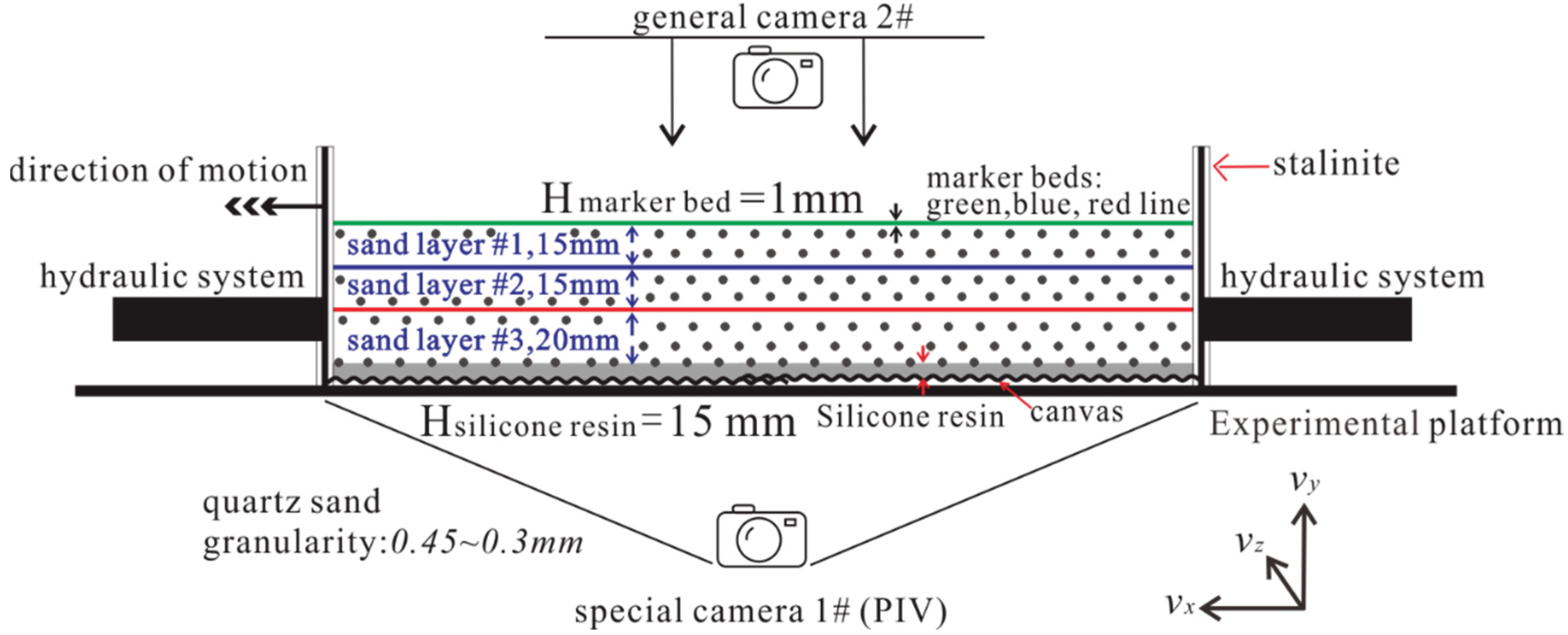
2.2. Experimental Setup

Figure 1 shows the experimental apparatus, which is a comprehensively experimental platform for the physical simulation of geological structural deformation, which is provided by the State Key Laboratory of Oil and Gas Reservoir Geology and Exploitation (Chengdu University of Technology). It includes a control system, a simulation chamber, a hydraulic system, a camera system, and a thermostat (air conditioner, with a temperature of 293.15 K).

The control system is used to control each system (including a simulation chamber, a hydraulic system, and a camera system) by computer (Figure 1). The simulation chamber is used to place dry quartz sands that simulates normal faults. Its size can be customized according to the experimental requirements, but it cannot be larger than 200 cm × 200 cm × 100 cm (length × width × height). The hydraulic system is used to provide tension or extrusion force with a maximum load of 10 kN and loading speed range of 0.0001 mm/s to 1 mm/s. The camera system includes a special camera 1# (PIV system, made by Beijing Cubetiandi Science and Technology Development Co., Ltd., Beijing, China) and a general camera 2# installed before and above the simulation chamber (Figure 2). The special camera 1# measures the displacement of the particles by processing the photo taking at 30-ms intervals. These photos are preprocessed using the Micro Vec 3 that comes with the PIV system and saved as digital format files (.dat); the digital format files can be opened using Tecplot. 360. 2010. The general camera 2# takes pictures of the experiment process and saves them.

We place the dry quartz sands in the simulation chamber, as shown in Figure 2. The hydraulic system provides tensions from the two ends of the simulation chamber. The recording system (the camera system) includes a special camera 1# (PIV system) and a general camera 2# installed before and above the simulation chamber, which is used to monitor the experiment continuously, as shown in Figure 2. The entire physical simulation is conducted at ambient conditions of 293.15 K, with the system temperature being maintained using a thermostat.

2.3. Experiment Procedure

The prototype of the normal fault in this study is from the Yanchang Formation of Jinhe oilfield, Ordos Basin, China, which has 289.31 million tons of oil-in-place and it is a vital development zone of the Sinopec North China Branch. The Jinhe Oilfield is located between Qingyang and Zhengning, where the area is 20 km × 17.5 km, as shown in Figure 3. Three Wells, JH 17, JH 62, and JH 64, have been drilled into this normal fault. The seismic interpretation and drilling indicate that this normal fault passes through the Yan’an, Yanchang and Ermaying Formation, and the thicknesses are 750 m, 750 m, and 1000 m, respectively; the Yanchang Formation sandstone is the main oil-producing layer in Jinhe Oilfield; the dip angle is in the range of 60°–65°; and, the fault displacement is falling in 30 m–45 m.

We set the experimental parameters following the similarity criterion between the model and prototype, including geometric, dynamic, and motion similarities [28,29,30]. Various similarity criteria are given, as follows:

(1) Geometric similarity. The area of the simulation chamber is 40 cm × 35 cm, while the area of the simulated strata is 20.0 km × 17.5 km with the geometric similarity ratio of L* = 2 × 10⁻⁵. The thicknesses of Yan’an, Yanchang, and Ermaying Formation in Jinghe Oilfield are 750 m, 750 m, and 1000 m, respectively. Therefore, we set the thicknesses of quartz sands in the simulation chamber as 15 mm, 15 mm, and 20 mm, respectively. Because the physical properties of the dry quartz sands do not change throughout the simulations, to facilitate the observation of structural deformation in the simulation chamber, millimeter-thick colored quartz sands are laid on each layer surface as a marker bed, as shown in Figure 3.

(2) Dynamic similarity. We use the density similarity ratio of ρ* = 0.5 and acceleration of gravity ratio of g* = 1, as presented in

Table 1. The experimental parameters between the model and prototype.

Parameters	Units	Model	Prototype	Similarity Ratio
geometric similarity (L*)	cm	40 (length)	20.0 × 105	2 × 10−5
		35 (width)	17.5 × 105	2 × 10−5
Density (ρ*)	kg/m3	1.35 × 10 3	2.7 × 103	0.5
acceleration of gravity (g*)	m/s 2	9.8	9.8	1
dynamic similarity (σ*)	σ* = ρ* × g* × L* = 0.5 × 1 × 2 × 10−5			1 × 10−5
coefficient of viscosity (η*)	Pa·s	1 × 104 (★)	1 × 1019 (★)	1 × 10−15
Kinematic similarity (v*)	v* = σ*/η* × L* = (1 × 10−5)/(1 × 10−15) × (2 × 10−5)			2 × 105

(^★) The viscosity coefficient of the silicone resin used to simulate the detachment layer is set as 1 × 10⁴ Pa·s in this experiment; the slip coefficient of sedimentary stratum is set as 1 × 10¹⁹ Pa·s [30,32,33].

. Consequently, the dynamic similarity ratio of σ* and kinematic similarity ratio v* are 1 × 10⁻⁵ and 2 × 10⁵, respectively.

(3) Kinematic similarity. Previous studies have shown that the detachment layers in the prototype slipped and deformed at a strain rate of 0.23 mm/year [31], so the uniform velocity of v = 1.5 µm/s is taken as the strain rate in our experiments based on the kinematic similarity ratio, as presented in Table 1.

We first layer-fill dry quartz sands in the simulation chamber, as shown in Figure 2. Subsequently, we fix the hydraulic system at the right end of the simulation chamber, while open the left end to stretch the canvas at the bottom of sand layers at a uniform velocity (v = 1.5 µm/s) until the occurrence of antithetic faults. The experimental phenomena are monitored by the general camera 2# and the special camera 1# (PIV system), which records data at a time interval of 30 ms. The entire experimental procedures are repeated three times for replicability.

2.4. Data Analysis

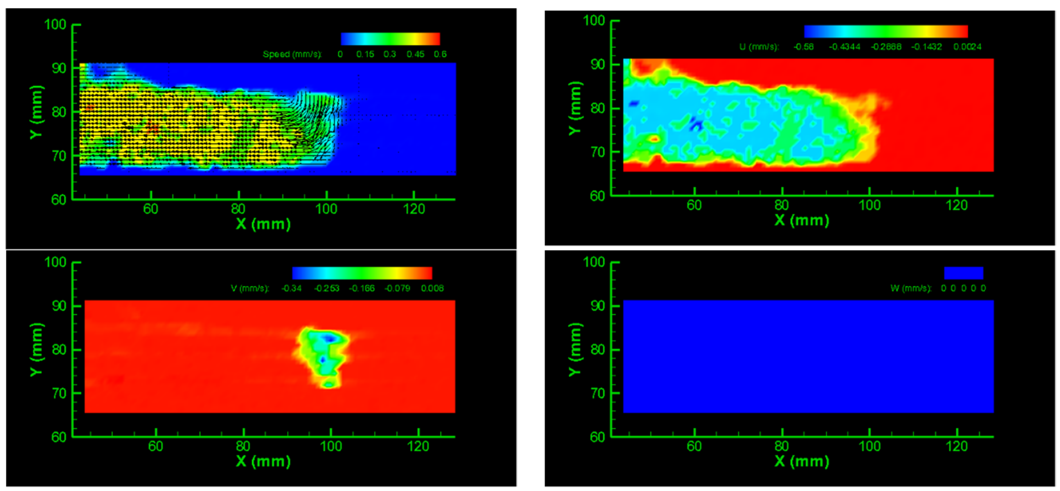
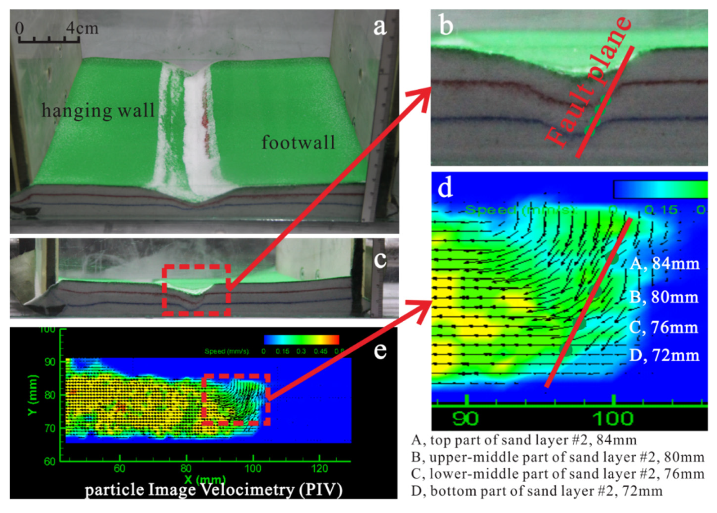
2.4.1. Data Collection by PIV Technique

The high-resolution Particle Image Velocimetry (PIV) is a technique, in which a series of images are obtained by a high-resolution special camera, and the velocity vectors of points are obtained by cross-correlation algorithms [34,35]. The PIV measurement can observe the whole dynamic process without disturbing the test object, and then obtain the instantaneous velocity profiles. The cross-correlation algorithms allow for the calculation of displacement vectors in the sand with sub-pixel accuracy (<0.1 pixels). With a given optical vector accuracy of better than 0.1 pixels, the absolute accuracy of the displacement vectors (dx) depends on the image scaling and correction [36].

In this study, the PIV system is from Beijing Cubetiandi Science and Technology Development Co., Ltd. (http://www.piv.com.cn, accessed on 1 April 2021) and has an optical resolution of 16 megapixels (4 k × 4 k) and a given optical vector accuracy of better than 0.5 pixels. In this experiment, with an optical resolution of 16 megapixels (4 k × 4 k) and an experiment with 40 cm width, the absolute accuracy of the length of displacement vectors is 0.1 mm. PIV is used to measure the displacement of the particles by processing the photos taken every 30 ms in this paper, as shown in Figure 4. Micro Vec 3 and Tecplot. 360. 2010 are the software used by the authors.

However, the inevitable micro-vibration of tempered glass baffles during the experiment and air disturbance on the top surface of sand layers in the simulated chamber would affect the experimental precision. In the actual analysis, the data within 2 cm near the glass baffle and within 1 cm of the top surface of sand layers in the simulated chamber are discarded. The data used for the analysis are between 85 mm and 110 mm in the x-coordinate and 70 mm and 90 mm in the y-coordinate. In addition, the hydraulic system takes about 30 min. to start and balance, so the initial recording time is from 2040 s to eliminate the systematic errors.

According to current metrological recommendations of GUM [37,38,39], every correctly performed measurement requires that its result be supplemented with a qualitative parameter characterizing this measurement, i.e., with the value of error or uncertainty.

To verify the accuracy of the measurement method and the measurement results by PIV, the velocity measurements at the center point (97.5 mm, 80 mm) of the simulation chamber were analyzed, as shown in Figure 4.

Table 2. The value of measurement uncertainty of PIV measured quantity.

Velocity [mm/s]	Mean	Standard Deviation	SE of Mean	Lower 95% CI of Mean	Upper 95% CI of Mean	Mean Absolute Deviation
total	0.439	0.03927	0.00674	0.42611	0.45341	0.03211
U	0.413	0.03171	0.00544	0.40247	0.42459	0.02685
V	0.145	0.03671	0.00629	0.13249	0.15811	0.03035

presents the information of standard deviation, standard error (SE) of mean, lower 95% confidence interval (CI) of mean, upper 95% CI of mean and mean absolute deviation values of 34 groups data of measurements for total velocity, U velocity, and V velocity by PIV. The result presented in Figure 2 shows that the measurement method and measurement results by the PIV technique can be compared with each other.

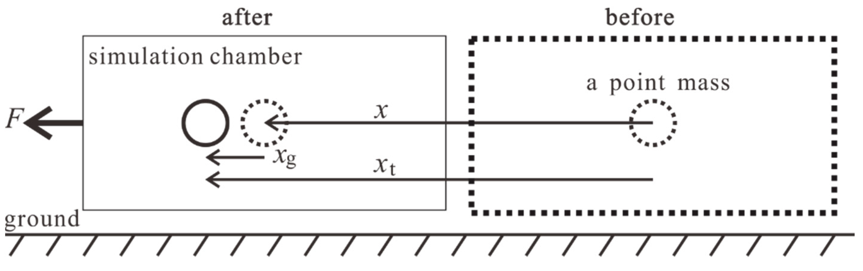
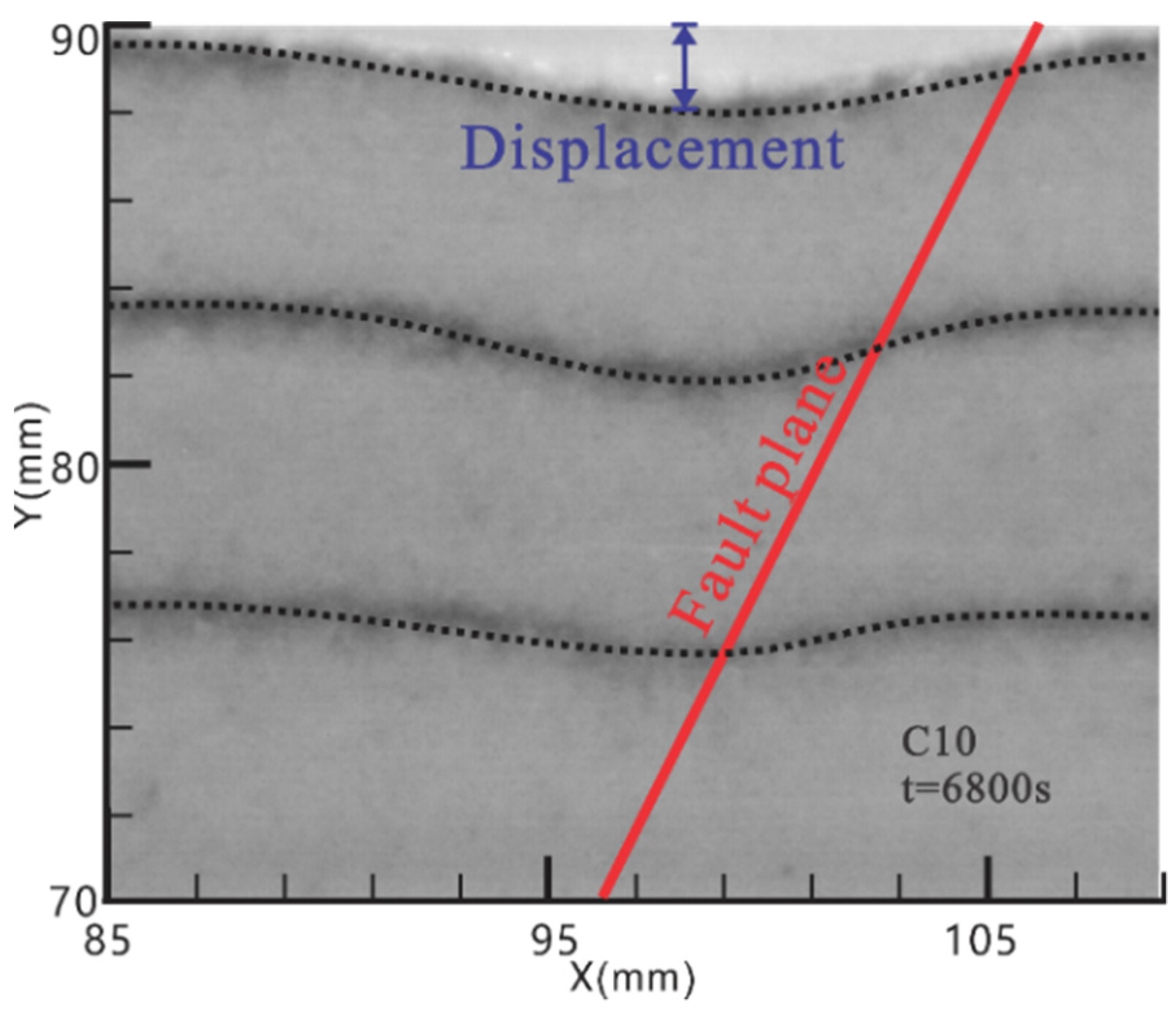
2.4.2. Dip Angle and Fault Displacement

The dip angle (α) in the unit of degree (°) is the angle between the normal fault line and horizontal projection line [40], which can be obtained as,

$$\alpha =\arctan \frac{v_y}{v_x}$$

(1)

where v_x and v_y are velocities in x- and y- coordinates in the unit of mm/s, respectively, where x- and z- are used as the directions in easting and northing, and y- would be the depth, as shown in Figure 2.

The sand layers in the simulation chamber are designed to be horizontally stressed, i.e., v_y = 0 mm/s, so that the dip angle is 0° or no dip angle is seen before the breakage of sand layers. α ≠ 0° indicates the fracture of sand layers. It is important to note that this is only true in this sandbox experiment.

In geology, a fault is a planar fracture or discontinuity in a volume of rock, across which there has been significant displacement as a result of rock-mass movement. This significant displacement is called fault displacement (L) [41], which can be calculated by,

$$L={\displaystyle \sum _{t=0}^{t=m}{L}_{i,j,\mathrm{t}}}={\displaystyle \sum _{t=0}^{t=m}(s_{i+1,j,t}-s_{i,j,t})={\displaystyle \sum _{t=0}^{t=m}(v_{i+1,j}-v_{i,j})t}}$$

(2)

where L is the fault displacement in the unit of m, S_i+1,j,t and S_i,j,t are the displacements of two adjacent points located on the same layer in the unit of m, v_i+1,j and v_i,j are the speeds of two adjacent points in the unit of m/s, and t is the total time in the unit of s.

2.4.3. Strain Energy and Strain Energy Density

Strain energy is the potential energy that is stored in strata in the form of strain and stress. Differential equations of motion in a single-degree-of-freedom system can only be transformed into energy balance equations under the horizontal tensile force [12]. Given a viscously damped single-degree-of-freedom system subjected to a horizontal earthquake ground motion, the equation of motion can be written as,

$$m{\ddot{x}}_t+c\dot{x}+f\left(x\right)=0$$

(3)

$$x_t=x+x_g$$

(4)

where m represents mass, c is the viscous damping coefficient, f(x) is the restoring force, x_t is the total displacement of the mass with respect to the ground, x is the displacement of the simulation chamber, and x_g is the relative displacement of the mass with respect to the simulation chamber, as shown in Figure 5.

Integrating Equation (3) with respect to x results in,

$${\displaystyle \int m{\ddot{x}}_{t}dx+}{\displaystyle \int c\dot{x}dx+}{\displaystyle \int f\left(x\right)dx=0}$$

(5)

Replacing x = x_t − x_g, in the first term of Equation (5), then

$${\displaystyle \int m{\ddot{x}}_{t}dx={\displaystyle \int m{\ddot{x}}_t\left(d{x}_{\mathrm{t}}-d{x}_g\right)={\displaystyle \int m\frac{{\dot{x}}_t}{dt}d{x}_t-{\displaystyle \int m{\ddot{x}}_{t}d{x}_g=m\frac{{\left({\dot{x}}_t\right)}^2}{2}-{\displaystyle \int m{\ddot{x}}_{t}d{x}_g}}}}}$$

(6)

Substituting Equation (6) into Equation (5) yields,

$$m\frac{{\left({\dot{x}}_t\right)}^2}{2}+{\displaystyle \int c\dot{x}dx+}{\displaystyle \int f\left(x\right)dx}={\displaystyle \int m{\ddot{x}}_{t}d{x}_g}$$

(7)

where $E_k=\frac{m{\left({\dot{x}}_t\right)}^2}{2}$ is the kinetic energy, $E_{\xi }=\int c\dot{x}dx$ is the damping energy, $E_a=\int f\left(x\right)dx$ is the absorbed energy, and $E_i=\int m{\ddot{x}}_{t}d{x}_g$ is the input energy.

We assume that the unit volume of rock has no heat exchange with the outside environment during the deformation process under external force, based on the first law of thermodynamics. Based on the first law of thermodynamics, we have

$$E_i=E_d+E_e$$

(8)

where: E_d is the unit dissipation, forming internal damage and shaping deformation, i.e., the change of internal state conforms to the trend of entropy increase; E_e is the unit released strain energy, in which the elastic strain energy can be released after unloading in strata [42].

Because the earth’s crust is an isothermal layer, we conduct the experimental data at a constant temperature without heat exchange. In other words, E_d = 0, so we have E_e as

$$E_e=E_i={\displaystyle \int m{\ddot{x}}_t}d{x}_g$$

(9)

The strain energy accumulated in the unit volume of strata is called the strain energy density [18], and it can be calculated as

$${\mathsf{\rho }}_e={\displaystyle \int }\frac{m}{V}{\ddot{x}}_{t}d{x}_g$$

(10)

where ${\mathsf{\rho }}_e$ is the unit released strain energy density and V is the unit volume.

The strain energy release rate (SERR) is an effective parameter to characterize normal fault formation and evolution [43]. In this study, the ratio of strain energy reduction to the total strain energy during the strain energy release process (E_eb > E_ea) is defined as the strain energy release rate that is given as [44],

$$SERR=\frac{E_{eb}-E_{ea}}{E_{eb}}\times 100\%$$

(11)

where E_eb is the total strain energy before the release and E_ea is the total strain energy after the release.

3. Results and Discussion

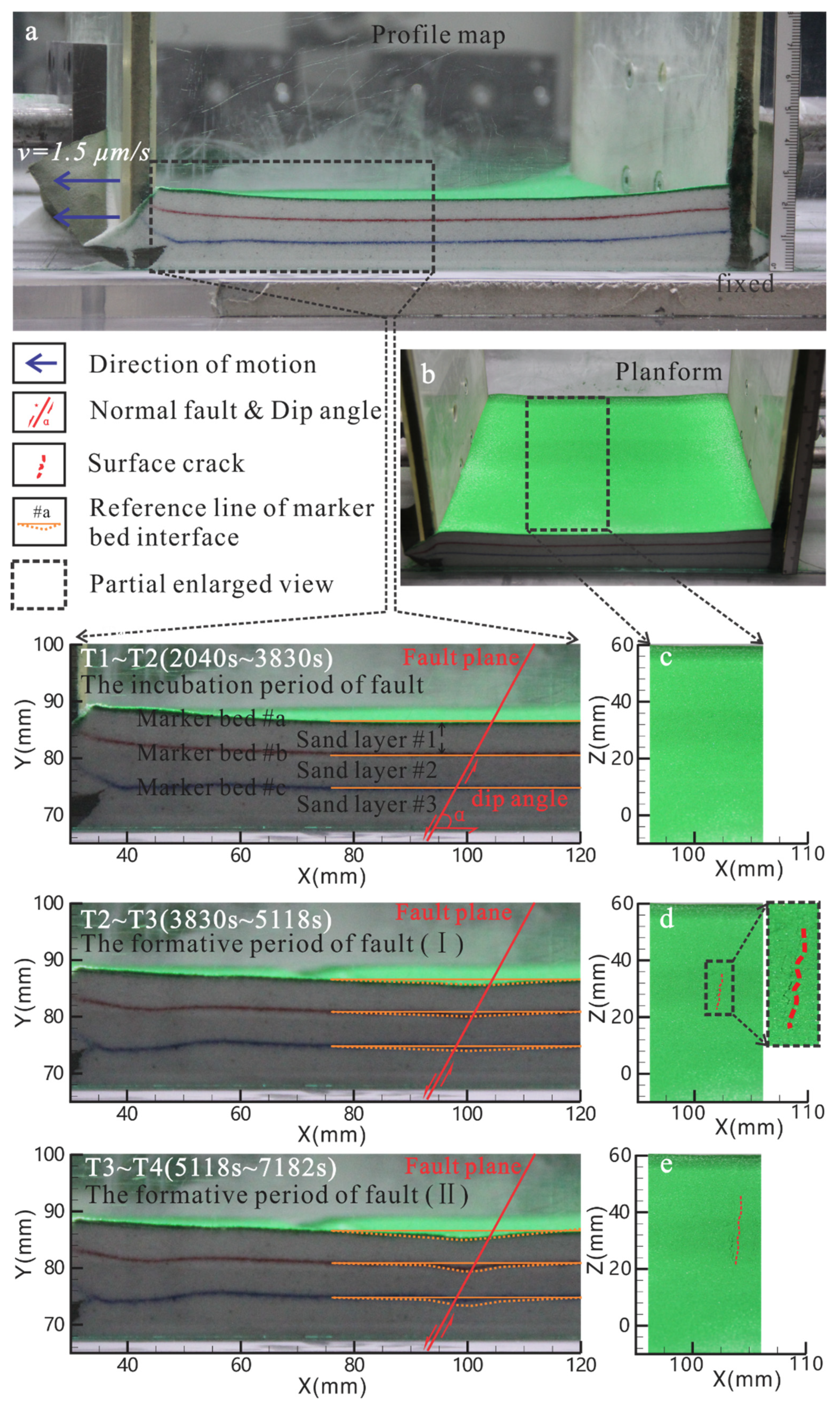
3.1. Identifying the Formation and Evolution of Normal Fault

In Figure 6, we present the digital image of the experimental procedures. The dry colored quartz sands laid on each layer surface comprise the marker bed, while track reflects the progress of normal fault tectonic deformation. The marker bed in the simulation chamber remains intact, and there is no sign of fracture from t = 2040 s to t = 3830 s, as shown in Figure 6. The marker bed is gradually bent to form the first depression and the vertical depression braking distance on the cross-section increases from t = 3830 s to t = 7426 s. Subsequently, a second depression forms from t = 7426 s to t = 8670 s. During the first depression period, the first micro-crack (the micro-crack refers to the fault line that can be seen on the top surface as shown in Figure 6) on the horizontal plane forms at t = 5118 s and the second at t = 7182 s. The length of the first micro-crack gradually increases until a distinct fault line forms on the horizontal plane from t = 5118 s to t = 7182 s and the second from t = 7182 s to t = 7426 s.

We depict the experimental phenomenon in detail and the calculated PIV, as shown in Figure 7. The triangular facet, which is the outcrop characteristic of the normal fault [45] can be observed in the simulation chamber. Generally, a fault line is a line that is commonly plotted on geologic maps to represent a fault and a fault plane where the fault can be seen or mapped on the surface. However, the fault plane is a plane that represents the fracture surface of a fault. In this study, we define the fault line as the localized shear zone, and the fault zone as the more distributed deformation around the localized shear zone. It is well known that the fault line is the central region of the normal fault that best reflects its formation and evolution. Four equally spaced recording points on the fault line are selected to analyze the dip angle and fault displacement change over time in this study.

According to the kinematic similarity (v* = 2 × 10⁵) seen in Table 1, the strain energy of normal fault in the experiment is converted into the energy of the real geological prototype, which is convenient to compare with the energy released when a real normal fault is formed. Figure 8 presents the strain energy that is obtained by Equation (9) between 85 mm and 110 mm in the x-coordinate and 70 mm and 90 mm in the y-coordinate from Figure 7d during the experiment.

The three repeated experiments show similar strain energy curves, as shown in Figure 9. As a result, we use the mean data of three experiments to illustrate the strain energy evolution, as shown in Figure 10 and Figure 11.

It is observed that the strain energy has a periodic variation of accumulation and release, conforming to the elastic rebound theory [46], which claims that the total strain energy that can be accumulated in the strata has a fixed upper limit, as shown in Figure 9. When such a limit is exceeded, the strata fracture will form normal fault and release strain energy. When the total strain energy stored in the strata declines to a certain low level, it begins to accumulate in a new cycle. Based on such strain energy evolution, we classify six different time intervals, as depicted in

Table 3. Time intervals during the formation and evolution of normal fault.

Timepoint	Time, s	Strain Energy, ×1013 J
T1	2040	0.0161
T2	3830	7.9011
T3	5118	4.7146
T4	7182	19.2356
T5	7426	22.7641
T6	8670	23.2352

. The first time interval, T1, is set at t = 2040 s, when the experiment starts; the second time interval, T2, is set at t = 3830 s, when the marker bed is bent to form the first depression; the third time interval, T3, is set at t = 5118 s, when the first micro-crack forms on the horizontal plane; the fourth time interval, T4, is set at t = 7182 s, when the second micro-crack forms on the horizontal plane; the fifth time interval, T5, is set at t = 7426 s, when the second depression forms; and, the sixth time interval, T6, is set at t = 8670 s, when the experiment ends. Overall, the formation and evolution of normal fault have distinct stages, which should be studied separately.

We depict the dip angle evolution during the third experiment in Figure 10. It shows that the dip angle is almost 0° and the sand layers do not have a fracture between T1 and T2. Between T2 and T3, the dip angle is between 0° and 3° and fracture occurs. Moreover, the dip angle increases sharply and can be up to 70° between T3 and T4. However, the dip angle shows a decreasing trend between T4 and T5, indicating that the normal fault activity begins to weaken, and it enters a stable stage. Between T5 and T6, the antithetic fault occurs with normal fault evolution, which is called the antithetic fault formation period. Additionally, we can find that the tendency of α decreases from the top part of sand layer #2 to bottom part of sand layer #2, indicating that, the shallower the buried depth of the sand layers, the more active normal fault.

Figure 11 presents the fault displacement of the normal fault. According to the geometric similarity (L* = 2 × 10⁻⁵) of Table 1, the fault displacement of the normal fault in the experiment is converted into the fault displacement of the real geological prototype, which is convenient to compare with the actual fault displacement. When the fault displacement is 0 mm, the sand layers do not fracture between T1 and T3, as shown in Figure 11. The fault displacement increases rapidly between T3 and T4, which is the main period of normal fault formation. The fault displacement tends to be stable between T4 and T5, indicating that the occurrence of antithetic fault weakens the normal fault activity. The fault displacement continues to increase during between T5 and T6, because the formation of the antithetic fault increases the total displacement. We can also find that the tendency of the fault displacement decreases from the top part of sand layer #2 to the bottom part of sand layer #2. The trend of the dip angle and fault displacement with buried depth is the same, showing that the activity of normal fault gradually increases as the buried depth increases.

According to the previous works [47,48], the dip angle, fault displacement, and strain energy characteristics, the formation and evolution of normal fault are divided into three distinct periods in this work: the incubation period, formative period, and antithetic fault period, as shown in

Table 4. The dividing basis of the formation and evolution of normal fault periods.

Items	Incubation Period	Formative Period			Antithetic Faults Period
		Elementary Stage	Unstable Stage	Stable Stage
time point (s)	T1~T2 (2040~3830)	T2~T3 (3830~5118)	T3~T4 (5118~7182)	T4~T5 (7182~7426)	T5~T6 (7426~8670)
dip angle (α, °)	almost 0	0~3	close to 70	decline	stable
fault displacement (L, m)	0	0	increase rapidly	stable	increase rapidly

.

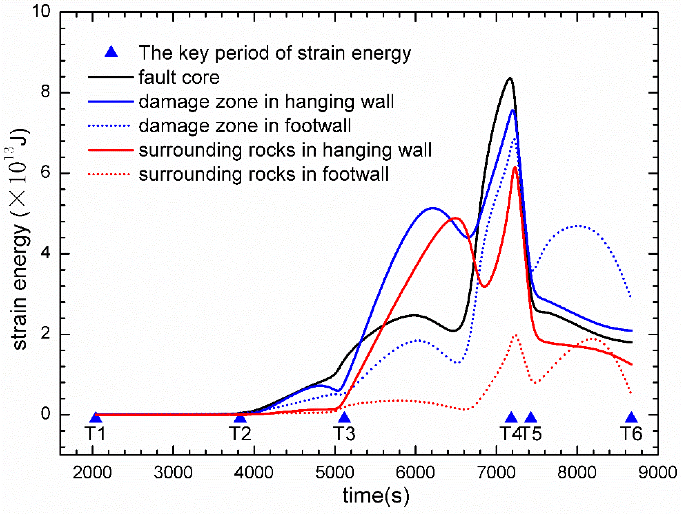
3.2. Strain Energy Density Variation during the Formation and Evolution of Normal Fault

In this section, we illustrate the variation of strain energy density in different periods of normal fault formation and evolution. The Surfer 12 software draws the contour maps of strain energy density.

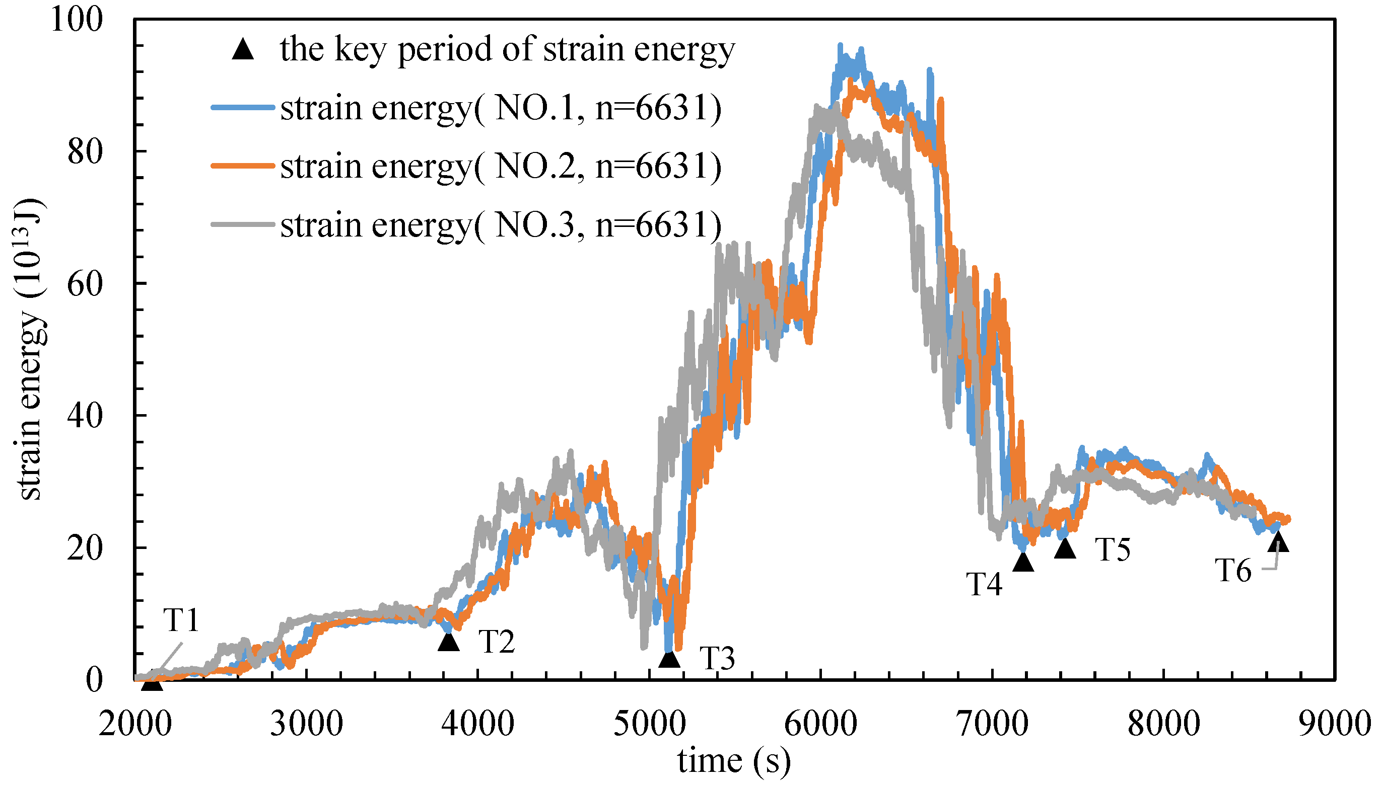
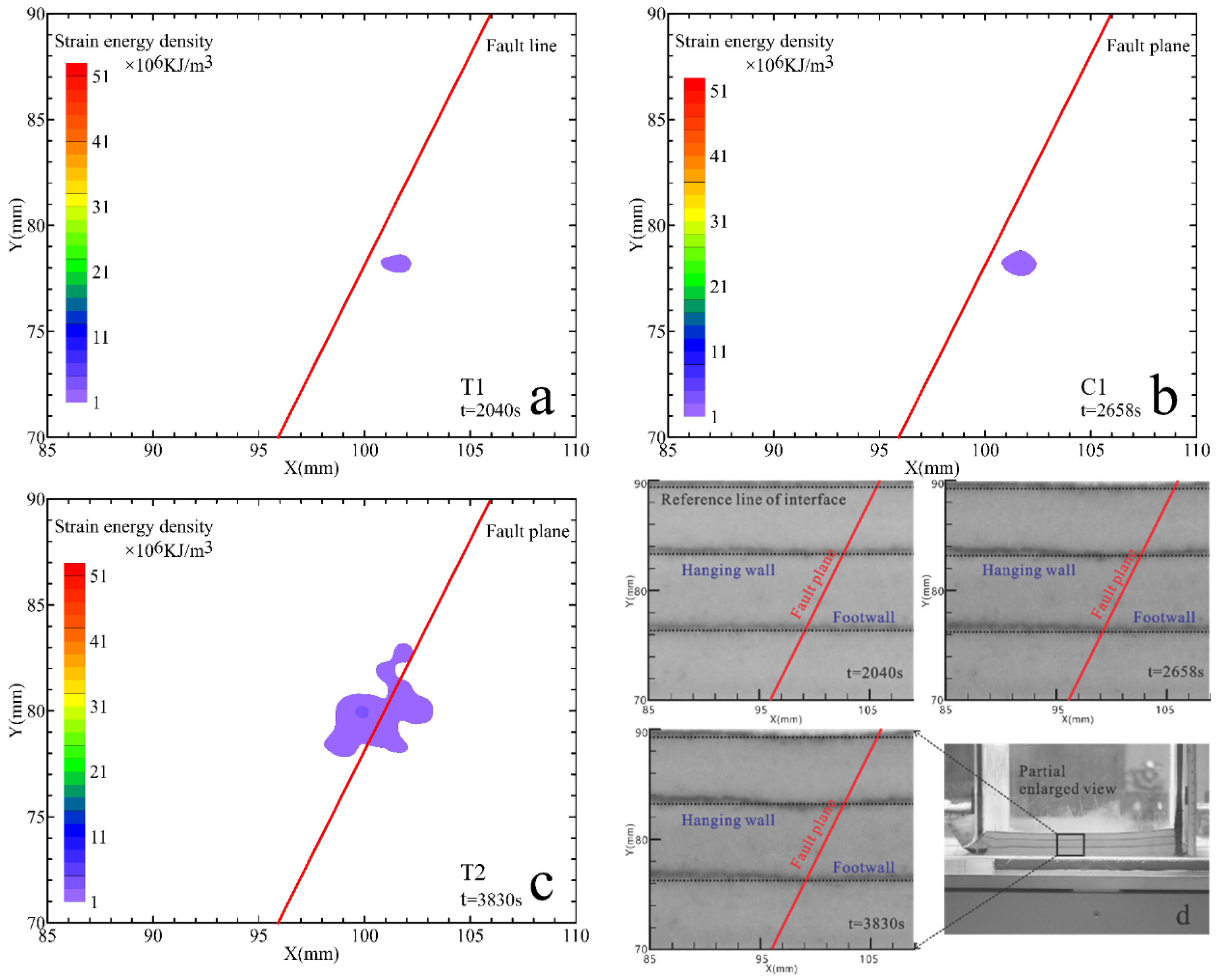
3.2.1. The Incubation Period (T1~T2)

During this period, the strain energy density increases gradually and slowly under the horizontal tectonic stress, as shown in Figure 12. The average strain energy density is less than 5 × 10⁶ KJ/m³, and the strata do not break to form a normal fault. The first region of strain energy accumulation forms and then expands below the fault line. As the structural stress continues, the strain energy accumulation occurs over the fault line. Finally, they merge to form the normal fault nucleation.

3.2.2. The Formative Period (T2~T5)

• The elementary stage (T2~T3)

During this stage, the strain energy density first increases and then decreases, as shown in Figure 13, and the average strain energy density is 10 × 10⁶ KJ/m³. The strain energy density of the fault line region increases fastest, reaches the limit of strata failure value E = 15 × 10⁶ KJ/m³, and then decreases first. Moreover, after that, the strain energy density of the hanging wall and footwall regions increases and forms two new strain energy accumulation regions, as shown in Figure 13c, and the strain energy density of the footwall reaches the limit of strata failure value E and is then released. The strain energy density of the hanging wall in the region (98 mm, 75 mm) is completely released at T3, as shown in Figure 13f,g. However, the sand layers in the simulation chamber remain stable, and the fault line does not appear, as shown in Figure 6d. We can conclude that the multi-region strain energy release is the precursor of normal fault formation.

2.

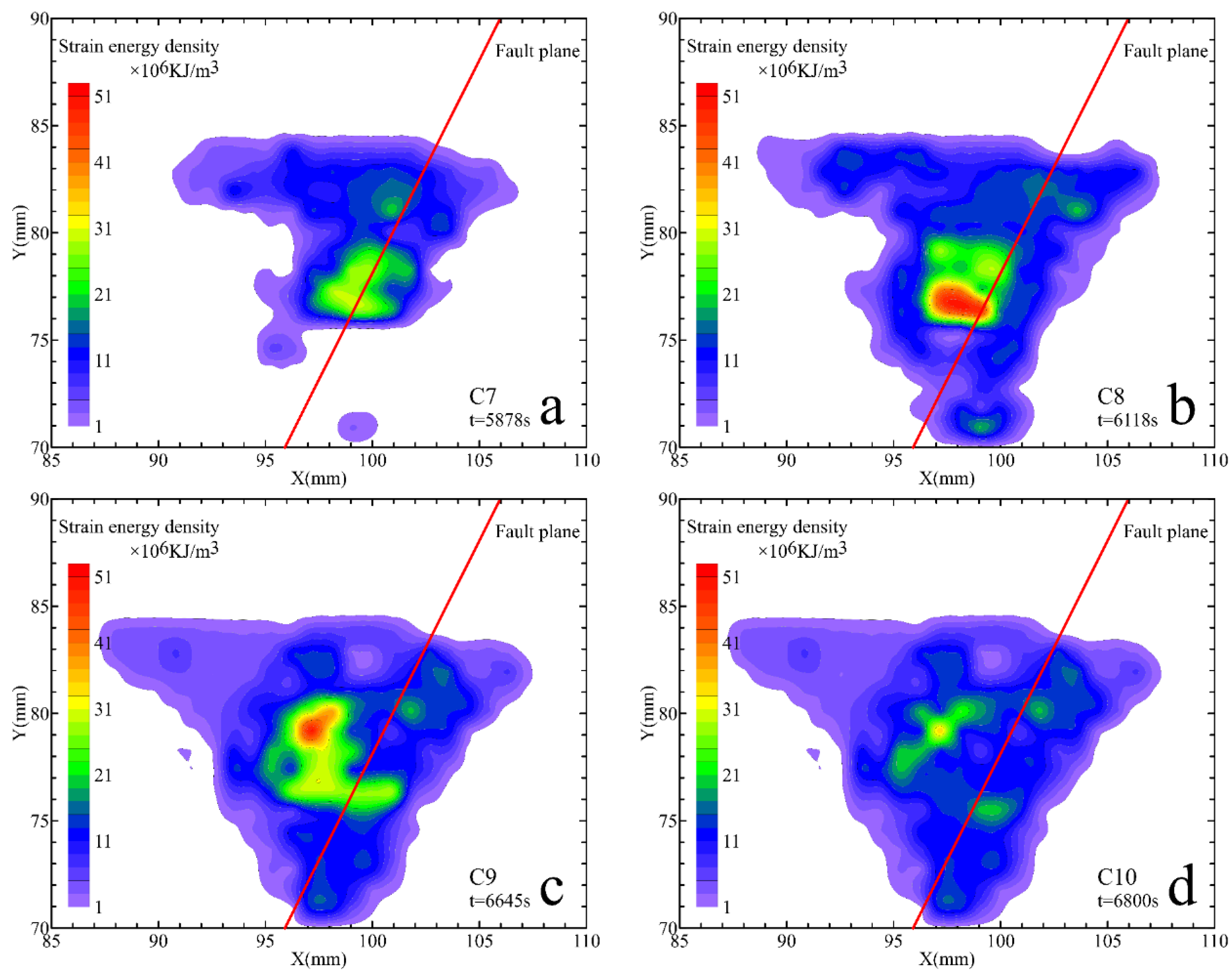
The unstable stage (T3~T4)

The strain energy is also accumulated before the release at this stage, as shown in Figure 14, but the average strain energy density is 20 × 10⁶ KJ/m³, which is quadruple that during the incubation stage. The strain energy of the hanging wall in the region (98 mm, 75 mm) is accumulated again, in a large area. A small area of strain energy accumulation region forms below the fault line and then merges into the large-scale one, which results in unstable strain energy density distribution in the layers. Figure 15 shows that the integrity of the fault zone is formed, and the fault line penetrates the strata. The main strain energy release occurs in the fault line zone, which is the reason for the fault line stability loss.

3.

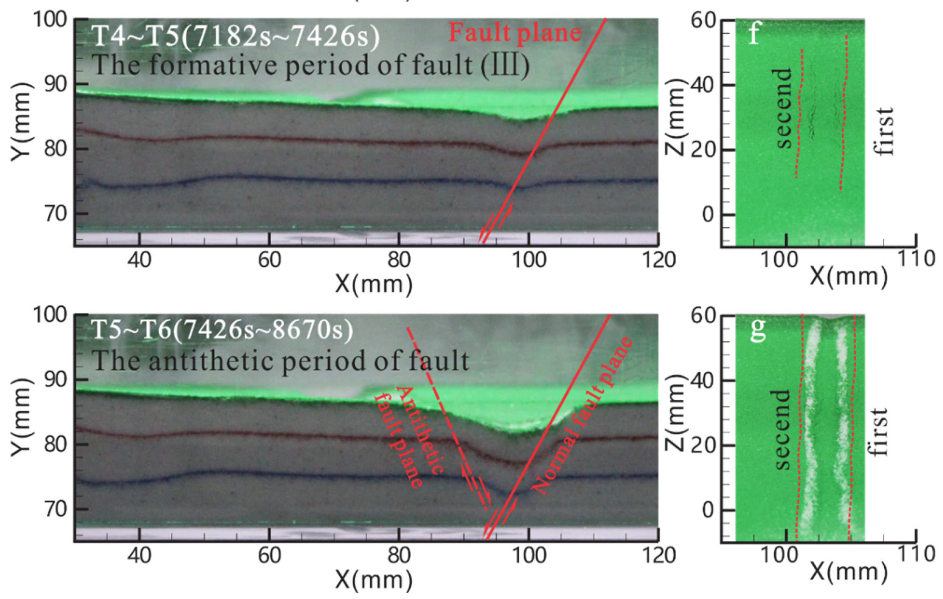
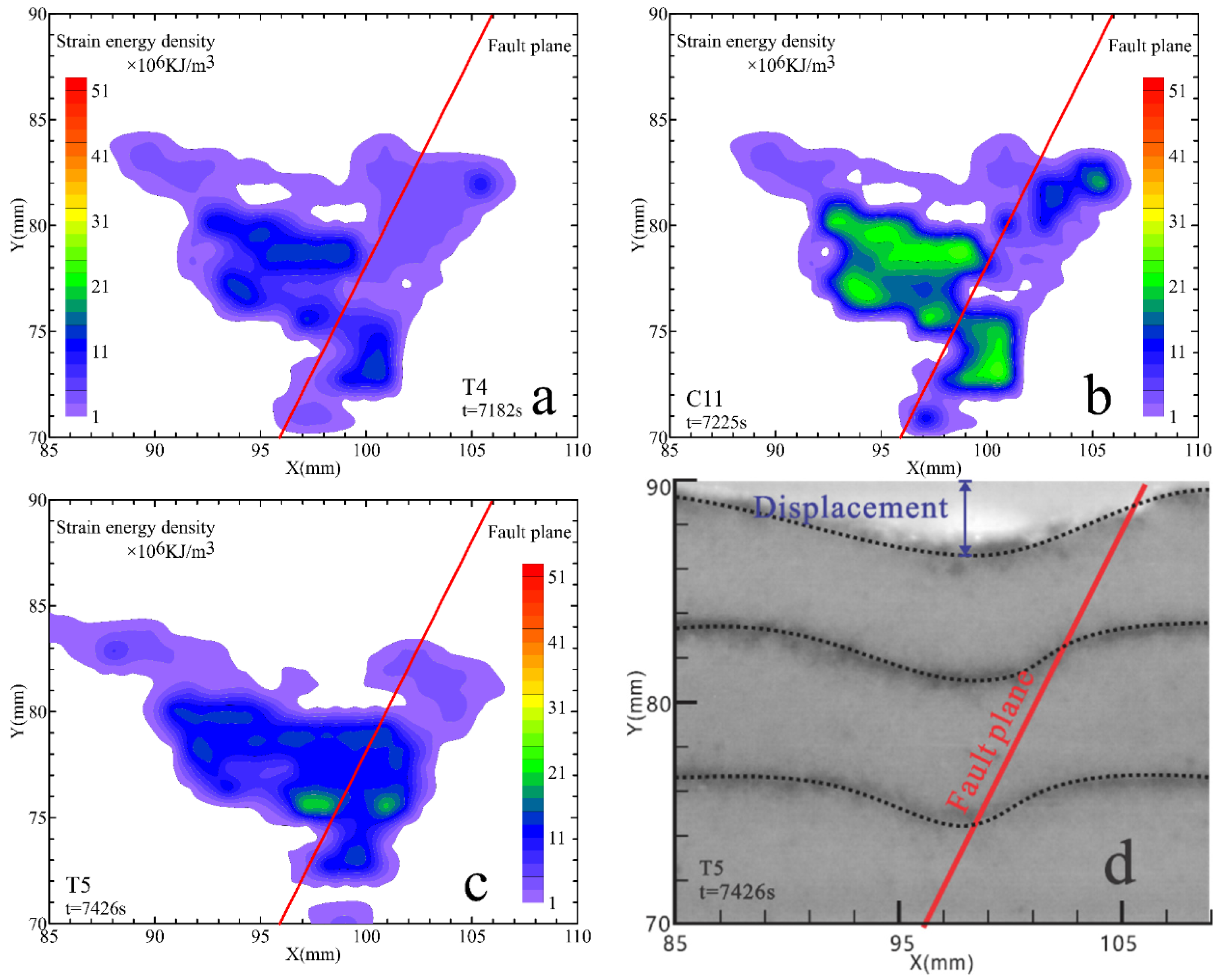
The stable stage (T4~T5)

A typical normal fault fracture zone structure is formed with the initiation of a fault line, a fault has formed. It then just continues to grow/propagate downwards at T5, as shown in Figure 16. The hanging wall moves past the footwall on the fault, which generates heat and dissipates strain energy. The amount of strain energy increase is equivalent to that of the released. The total strain energy tends to be stable, and the normal fault is in a stable period.

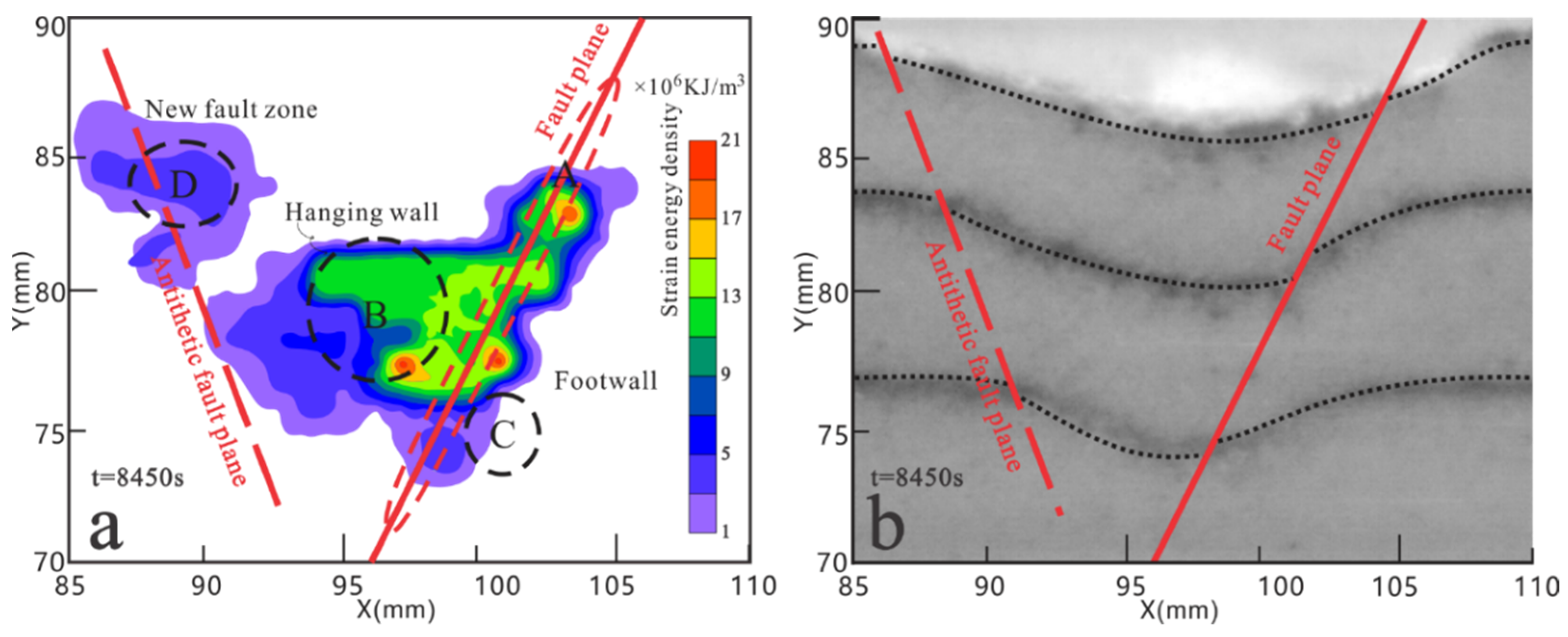
3.2.3. The Antithetic Fault Period (T5~T6)

Figure 17 shows that the fault lines cut off the connection between the hanging wall and footwall layers after flexure. The footwall is no longer subjected to the horizontal tectonic stress, and its strain energy gradually becomes stable. However, the hanging wall has been under structural stress, and its strain energy increases again after a short period of stability. As the strain energy of the hanging wall reaches the limit of strata failure value, the antithetic faults form in a region that is far from the fault line on the hanging wall. Moreover, the residual strain energy after the formation of normal fault is mainly located on the hanging wall, which is also the cause of the instability of the hanging wall.

3.2.4. The Strain Energy of Each Period

The average strain energy density at different periods has the following characteristics. The average strain energy density of the elementary stage is twice as big as the one of the incubation periods. The one at the stable stage is larger than the one at the antithetic fault period. The one at the unstable stage is 20 × 10⁶ KJ/m³, which is the largest among them. Therefore, the average strain energy density can be used as an indicator of normal fault formation and evolution.

Figure 18 presents that the different regions of strata have different strain energy density characteristics. The strain energy density in the hanging wall is larger than that of the footwall, which is only 75% of the hanging wall. The strain energy is mainly located in region B of the hanging wall, the C region of the footwall, and D region, where the antithetic fault is formed. The strain energy in the A region near the fault line is the biggest. The strain energy density has the characteristic that, the farther away from the fault line, the smaller it is in the footwall and the upper 10 mm of the hanging wall.

3.3. Strain Energy Characteristics of Normal Fault

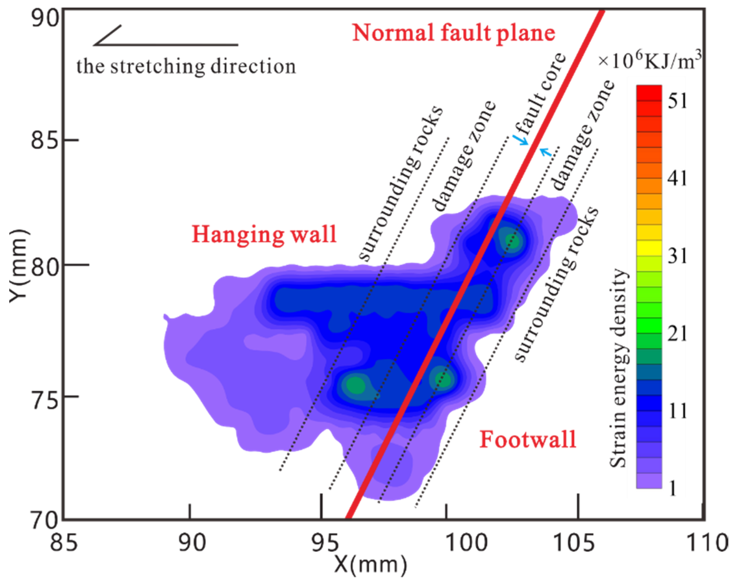
3.3.1. Distribution of Strain Energy Density

The strain energy distributions in the hanging wall and footwall are different, as shown in Figure 19. Thus, in this study, the normal fault zone is divided into five regions, namely the fault cores, damage zone in the hanging wall, damage zone in the footwall [49], surrounding rocks in the hanging wall, and surrounding rocks in the footwall, as shown in Figure 19. According to the previous achievements of the normal fault zone of Yanchang Formation in the Jinghe Oilfield, the distribution range of each region is known according to the geometric similarity ratio L*, as shown in

Table 5. Range conversion table for each region of the normal fault in the prototype and experiment (L* = 2 × 10⁻⁵).

Normal Fault Zones	Range in the Prototype, m	Range in the Model, mm
Fault core	(0, 50]	(0, 1]
damage zone in the hanging wall	(50, 140]	(1, 2.8]
damage zone in the footwall	(50, 125]	(1, 2.5]
Surrounding rocks in the hanging wall	(140, ∞)	(2.8, ∞)
Surrounding rocks in the footwall	(125, ∞)	(2.5, ∞)

.

Figure 20 shows that the five regions have similar strain energy characteristics. The strain energy of each region gradually increases during the incubation period. The strain energy of each region has a similar feature to increasing first and then decreasing. Among them, the normal fault core has the largest strain energy, and the rupture zone in the hanging wall is second during the elementary stage. The strain energy increases significantly after a brief decrease in all five regions, and the strain energy increases at the fastest rate in the region of the rupture zone in the hanging wall. The strain energy is reduced in all five regions during the stable stage. The strain energy begins to decrease after a brief increase in the surrounding rock in the hanging wall during the antithetic fault period.

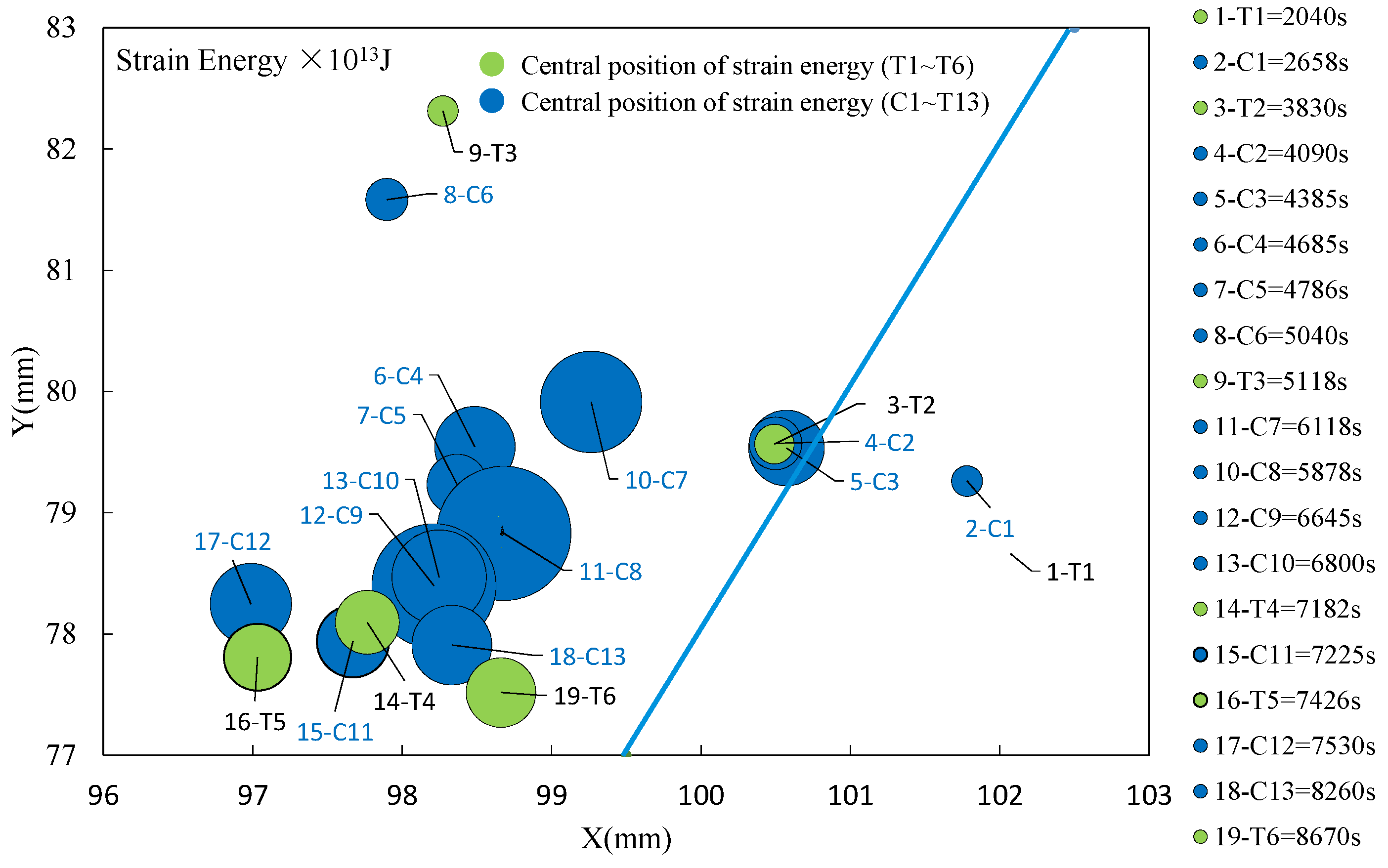
3.3.2. The Central Position of Strain Energy

In general, the energy source causing the tectonic deformation of the strata cannot be assumed as a point source. The size of structural deformation does not significantly affect the energy attenuation direction of normal fault. Therefore, the energy source of a normal fault can be assumed to be a point source [49]. Calculating the position of the energy source that causes the formation to generate a normal fault based on the material point method, also known as the central position of strain energy (CPSE). In this work, the CPSE is calculated by Equation (A8) in Appendix A and shown in Figure 21. The area of the dot represents the magnitude of the strain energy at each time point (19 in total), and the position of the dot represents the position of the strain energy at each time point, as shown in Figure 21. The CPSE is mainly located in the fault line and the hanging wall, and its position and magnitude change with time, as following: the CPSE is located at the bottom of the footwall and moving to the fault line during the incubation period, while it is located at the fault line during the elementary stage. As the strain energy reaches the limit of strata value and is released, the CPSE jumps from the fault line to the hanging wall. The strain energy release results in an unstable state of the hanging wall, forming a new CPSE. The CPSE moves to the depth of the hanging wall during the stable stage, while it moves to the bottom position of the fault line, and the strain energy first increases and then decreases during the antithetic fault period.

The CPSE change with time indicates that the location of the fracture is not fixed during normal fault formation and evolution. The fracture mainly occurs in the hanging wall, especially at the bottom of the hanging wall. The fracture at the bottom creates space, and the sands at the top of the strata collapse under gravity to replenish the missing space. The constant transformation of the CPSE is the reason why the associated fracture of the normal fault has both tension and shear cracks. The Anderson model of fault analysis from the perspective of triaxial force cannot explain this phenomenon. It is necessary to study the normal fault formation and evolution from the perspective of strain energy.

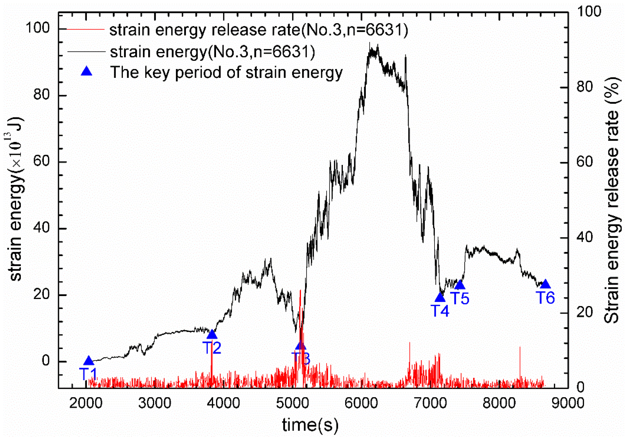
3.3.3. Strain Energy Release Rate

Figure 22 shows the strain energy release rate during normal fault formation. There is always strain energy release during the normal fault formation, but the release rate of strain energy is low, with a maximum value of 26.1% and an average value of 1.7%. The moment of strain energy release rate higher than average corresponds to the critical period of a normal fault (refers to T1–T6, as shown in Table 3). Therefore, the strain energy release rate is an indicator of the further evolution of normal fault. During the formation of a normal fault, the strain energy release rate has no relationship with the fracturing activity in the layers. On the one hand, the strain energy release rate during the normal fault formation period does not increase significantly, so the low strain energy release rate will not dictate that the layer fracture activity is weakened. On the other hand, the strain energy release rate increases significantly during the period before the stabilization period, which indicates that the sustained increase of the strain energy release rate is an indicator that normal fault is about to enter a stable period.

4. Discussion

Strain energy is one of the parameters that describes the strength of tectonic activity. Thus, the formation and evolution of (normal) fault can be studied by analyzing the variation of strain energy in stratas. Physical simulation experiments can only simulate the structural deformation under various conditions, but they cannot simulate basins and structures through direct visualization [20,21,22]. Therefore, we cannot study the formation and evolution of normal faults by this approach. In this paper, we use high-resolution particle imaging velocimetry (PIV), which can continuously monitor the experimental procedures, and the strain energy is calculated based on the velocity field of quartz sand particles, which is recorded by PIV. A case study in Yanchang Formation is presented to demonstrate the efficiency of the proposed method. The validation results prove that the approach in this paper could effectively and accurately explain the tectonic deformation of normal faults. As a result, the strain energy is mainly released in the normal fault line zone and, thus, can serve as channels for oil/gas migration and escape conduits connecting to the earth’s surface, destroying the already formed oil/gas reservoirs. Besides, a large amount of strain energy remaining in the hanging wall is the reason why the normal fault continues to evolve after the normal fault formation until the antithetic fault forms. One might need to avoid drilling near the fault line. More importantly, this paper may give a new perspective to study the formation and evolution of normal faults.

5. Conclusions

In this study, we used physical simulation experiments with PIV technology to study the formation and evolution of normal fault from the strain energy perspective. The following conclusions are drawn.

(1) The formation and evolution of normal faults are phased. We identified three phases, including the include incubation period, the formative period, and the antithetic fault period. During the incubation period, strain energy accumulates along the fault line, while it is generally small, and the strata are not broken. During the formative period, strain energy increases significantly, and it reaches the limit of strata and that in the fault line region is released, and normal fault tends to be in a stable stage. When the fault line cuts off the connection between the footwall and hanging wall before the antithetic fault period, the footwall is in a stable period, and the hanging wall would continue to move to form the antithetic fault period.

(2) Overall, the strain energy before normal fault formation is continuously accumulated. The normal fault is formed when the strain energy reaches the limit of strata. A low level of strain energy release randomly distributed cannot form normal faults. The main strain energy release occurs in the fault line zone. Consequently, one might need to avoid drilling near the fault line, but on the normal fault zone. The strain energy is released during the whole process of normal fault formation, and the maximum release rate is 26.1%. However, the low rate of strain energy release does not mean that the fault activity is weakened, and the sustained increase of strain energy release rate is a sign that the normal fault is about to enter a stable period.

(3) The average strain energy density is an indicator of the formation and evolution of normal fault. The farther from the fault line, the smaller the strain energy density. The influence range of the strain energy in the hanging wall is greater than that of the footwall. A large amount of strain energy remaining in the hanging wall is the reason why the normal fault continues to evolve after the normal fault formation until the antithetic fault is formed.

References

1. Wernicke, B.; Axen, G.J. On the role of isostasy in the evolution of normal fault systems. Geology 1988, 16, 848–851. [Google Scholar] [CrossRef]
2. Martinsen, O.J.; Pulham, A.J.; Haughton, P.D.; Sullivan, M.D. Outcrops Revitalized: Tools, Techniques and Applications; SEPM Tulsa: Tulsa, OK, USA, 2011. [Google Scholar]
3. Sibson, R. Fault rocks and fault mechanisms. J. Geol. Soc. 1977, 133, 191–213. [Google Scholar] [CrossRef]
4. Bernabé, Y.; Revil, A. Pore-scale heterogeneity, energy dissipation and the transport properties of rocks. Geophys. Res. Lett. 1995, 22, 1529–1532. [Google Scholar] [CrossRef]
5. Sujatha, V.; Kishen, J.C. Energy release rate due to friction at bimaterial interface in dams. J. Eng. Mech. 2003, 129, 793–800. [Google Scholar] [CrossRef]
6. Zhao, Z. Research on Rock Deformation and Failure Based on Energy Dissipation and Energy Release; Sichuan University: Chengdu, China, 2007. [Google Scholar]
7. Zhao, Z.; Lu, R.; Zhang, G. Analysis on Energy Transformation for Rock in the Whole Process of Deformation and Fracture. Min. Res. Dev. 2006, 26, 8–11. [Google Scholar]
8. Faulkner, D.; Jackson, C.; Lunn, R.; Schlische, R.; Shipton, Z.; Wibberley, C.; Withjack, M. A review of recent developments concerning the structure, mechanics and fluid flow properties of fault zones. J. Struct. Geol. 2010, 32, 1557–1575. [Google Scholar] [CrossRef]
9. Fajfar, P.; Vidic, T.; Fischinger, M. Seismic demand in medium and long period structures. Earthq. Eng. Struct. Dyn. 1989, 18, 1133–1144. [Google Scholar] [CrossRef]
10. Sucuoglu, H. Effect of connection rigidity on seismic response of precast concrete frames. PCI J. 1995, 40, 94–103. [Google Scholar] [CrossRef]
11. Teran-Gilmore, A. Performance-Based Earthquake-Resistant Design of Framed Buildings Using Energy Concepts; University of California: Berkeley, CA, USA, 1996. [Google Scholar]
12. Uang, C.M.; Bertero, V.V. Evaluation of seismic energy in structures. Earthq. Eng. Struct. Dyn. 1990, 19, 77–90. [Google Scholar] [CrossRef]
13. Akiyama, H. Earthquake Resistant Limit State Design for Buildings; University of Tokyo Press: Tokyo, Japan, 1985. [Google Scholar]
14. Holt, W.; Chamot Rooke, N.; Le Pichon, X.; Haines, A.; Shen Tu, B.; Ren, J. Velocity field in Asia inferred from Quaternary fault slip rates and Global Positioning System observations. J. Geophys. Res. Solid Earth 2000, 105, 19185–19209. [Google Scholar] [CrossRef]
15. Iinuma, T.; Ohzono, M.; Ohta, Y.; Miura, S. Coseismic slip distribution of the 2011 off the Pacific coast of Tohoku Earthquake (M 9.0) estimated based on GPS data—Was the asperity in Miyagi-oki ruptured? EarthPlanets Space 2011, 63, 24. [Google Scholar] [CrossRef] [Green Version]
16. Jing, Y.; Li, H.; Xiong, Y.Z.; Fan, L.L.; Zhang, S.Z.; Sun, Q.-W.; Dong, J.Y.; Liu, F.-Q.; Wang, H.-Z. Use Seismic Moment Tensor and GPS Data to Analyse the Recent CrustalM ovement Energy Distribution Characteristics of China Continent. Geol. J. China Univ. 2009, 1, 011. [Google Scholar]
17. He, M.; Miao, J.; Feng, J. Rock burst process of limestone and its acoustic emission characteristics under true-triaxial unloading conditions. Int. J. Rock Mech. Min. Sci. 2010, 47, 286–298. [Google Scholar] [CrossRef]
18. Sih, G.C. Strain energy density factor applied to mixed mode crack problems. Int. J. Fract. 1974, 10, 305–321. [Google Scholar] [CrossRef]
19. Young, W.C.; Budnyas, R.G. Roark’s Formulas for Stress and Strain; McGraw-Hill: New York, NY, USA, 2017. [Google Scholar]
20. Gutscher, M.A.; Klaeschen, D.; Flueh, E.; Malavieille, J. Non-Coulomb wedges, wrong-way thrusting, and natural hazards in Cascadia. Geology 2001, 29, 379–382. [Google Scholar] [CrossRef]
21. Lohrmann, J.; Kukowski, N.; Adam, J.; Oncken, O. The impact of analogue material properties on the geometry, kinematics, and dynamics of convergent sand wedges. J. Struct. Geol. 2003, 25, 1691–1711. [Google Scholar] [CrossRef]
22. Waltham, D. Folding and faulting in coulomb materials. Basin Res. 2002, 14, 319–328. [Google Scholar] [CrossRef]
23. Cloos, E. Experimental analysis of Gulf Coast fracture patterns. AAPG Bull. 1968, 52, 420–444. [Google Scholar]
24. McClay, K. Extensional fault systems in sedimentary basins: A review of analogue model studies. Mar. Pet. Geol. 1990, 7, 206–233. [Google Scholar] [CrossRef]
25. De Pater, C.; Cleary, M.; Quinn, T.; Barr, D.; Johnson, D.; Weijers, L. Experimental verification of dimensional analysis for hydraulic fracturing. SPE Prod. Facil. 1994, 9, 230–238. [Google Scholar] [CrossRef]
26. Bonini, M.; Corti, G.; Ventisette, C.D.; Manetti, P.; Mulugeta, G.; Sokoutis, D. Modelling the lithospheric rheology control on the Cretaceous rifting in West Antarctica. Terra Nova 2007, 19, 360–366. [Google Scholar] [CrossRef]
27. Costa, E.; Vendeville, B. Experimental insights on the geometry and kinematics of fold-and-thrust belts above weak, viscous evaporitic décollement. J. Struct. Geol. 2002, 24, 1729–1739. [Google Scholar] [CrossRef]
28. Hubbert, M.K. Theory of scale models as applied to the study of geologic structures. Bull. Geol. Soc. Am. 1937, 48, 1459–1520. [Google Scholar] [CrossRef]
29. Bonini, M. Deformation patterns and structural vergence in brittle–ductile thrust wedges: An additional analogue modelling perspective. J. Struct. Geol. 2007, 29, 141–158. [Google Scholar] [CrossRef]
30. Cotton, J.T.; Koyi, H.A. Modeling of thrust fronts above ductile and frictional detachments: Application to structures in the Salt Range and Potwar Plateau, Pakistan. Geol. Soc. Am. Bull. 2000, 112, 351–363. [Google Scholar] [CrossRef]
31. Xu, S.; Fukuyama, E.; Yamashita, F.; Mizoguchi, K.; Takizawa, S.; Kawakata, H. Strain rate effect on fault slip and rupture evolution: Insight from meter-scale rock friction experiments. Tectonophysics 2018, 733, 209–231. [Google Scholar] [CrossRef]
32. Couzens-Schultz, B.A.; Vendeville, B.C.; Wiltschko, D.V. Duplex style and triangle zone formation: Insights from physical modeling. J. Struct. Geol. 2003, 25, 1623–1644. [Google Scholar] [CrossRef]
33. Leturmy, P.; Mugnier, J.; Vinour, P.; Baby, P.; Colletta, B.; Chabron, E. Piggyback basin development above a thin-skinned thrust belt with two detachment levels as a function of interactions between tectonic and superficial mass transfer: The case of the Subandean Zone (Bolivia). Tectonophysics 2000, 320, 45–67. [Google Scholar] [CrossRef]
34. Adam, J.; Urai, J.; Wieneke, B.; Oncken, O.; Pfeiffer, K.; Kukowski, N.; Lohrmann, J.; Hoth, S.; Van Der Zee, W.; Schmatz, J. Shear localisation and strain distribution during tectonic faulting—New insights from granular-flow experiments and high-resolution optical image correlation techniques. J. Struct. Geol. 2005, 27, 283–301. [Google Scholar] [CrossRef]
35. White, D.; Take, W.; Bolton, M. Soil deformation measurement using particle image velocimetry (PIV) and photogrammetry. Geotechnique 2003, 53, 619–631. [Google Scholar] [CrossRef]
36. White, D.J.; Take, W.; Bolton, M. Measuring soil deformation in geotechnical models using digital images and PIV analysis. In Proceedings of the International Conference on Computer Methods and Advances in Geomechanics, Tucson, AZ, USA, 7–12 January 2001; pp. 997–1002. [Google Scholar]
37. Guide to the Expression of Uncertainty in Measurement, Joint Committee for Guides in Metrology (JCGM) 100:2008. Available online: https://www.bipm.org/documents/20126/2071204/JCGM_100_2008_E.pdf/cb0ef43f-baa5-11cf-3f85-4dcd86f77bd6 (accessed on 5 September 2008).
38. Golijanek-Jędrzejczyk, A.; Mrowiec, A.; Hanus, R.; Zych, M.; Świsulski, D. Uncertainty of mass flow measurement using centric and eccentric orifice for Reynolds number in the range 10,000 ≤ Re ≤ 20,000. Measurement 2020, 160, 107851. [Google Scholar] [CrossRef]
39. Golijanek-Jędrzejczyk, A.; Mrowiec, A.; Hanus, R.; Zych, M.; Świsulski, D. Determination of the uncertainty of mass flow measurement using the orifice for different values of the Reynolds number. Eur. Phys. J. Conf. 2019, 213, 02022. [Google Scholar] [CrossRef]
40. Lahee, F.H. Field Geology; McGraw-Hill Book Company, Incorporated: New York, NY, USA, 1923. [Google Scholar]
41. Newmark, N.M.; Hall, W.J. Pipeline design to resist large fault displacement. In Proceedings of the US National Conference on Earthquake Engineering, Ann Arbor, MI, USA, 18–20 June 1975; pp. 416–425. [Google Scholar]
42. Solecki, R.; Conant, R.J. Advanced Mechanics of Materials; Oxford University Press: New York, NY, USA, 2003; Volume 198. [Google Scholar]
43. Ding, Y.; Zhu, X. Probe into Input Energy for the Characterization of Earthquake Ground Motions. J. Beijing Jiaotong Univ. 2007, 31, 49–51. [Google Scholar]
44. Hussain, M.; Pu, S.; Underwood, J. Strain energy release rate for a crack under combined mode I and mode II. In Fracture Analysis: Proceedings of the 1973 National Symposium on Fracture Mechanics; Part II; ASTM International: West Conshohocken, PA, USA, 1974. [Google Scholar]
45. Ye, Q.; Yuan, M. Explanations of Common Terms in Oil and Gas Field Development; Petroleum Industry Press: Conshohocken, PA, USA, 1996. [Google Scholar]
46. Reid, H.F. The mechanics of the earthquake. In The California Earthquake of April 18, 1906, Report of the State Earthquake Investigation Commission; The Caknegie Institution of Washington: Washington, DC, USA, 1910. [Google Scholar]
47. Caine, J.S.; Evans, J.P.; Forster, C.B. Fault zone architecture and permeability structure. Geology 1996, 24, 1025–1028. [Google Scholar] [CrossRef]
48. Doughty, P.T. Clay smear seals and fault sealing potential of an exhumed growth fault, Rio Grande rift, New Mexico. AAPG Bull. 2003, 87, 427–444. [Google Scholar] [CrossRef]
49. Zhang, L.; Lv, Y.; Peng, Y.; Xie, Z. Analysis of Seismological Energy Density of Minor-moderate Earthquakes. Earthq. Res. China 2008, 24, 407–414. [Google Scholar]
Figure 1. The comprehensively experimental platform for physical simulation of geological structural deformation.
Energies 14 02825 g001
Figure 2. The schematic representation of the simulation chamber.
Energies 14 02825 g002
Figure 3. Prototype of physical simulation of geological structural deformation experiment. (a) The geographical position; (b) The seismic interpretation section of Jinhe Oilfield.
Energies 14 02825 g003
Figure 4. The instantaneous velocity profiles of the particles measured by the PIV technique (U, V, and W are the velocities in x-, y- and z-coordinates, respectively).
Energies 14 02825 g004
Figure 5. The relationship between x, xt, and xg.
Energies 14 02825 g005
Figure 6. Experimental phenomenon of a physical simulation experiment.
Energies 14 02825 g006aEnergies 14 02825 g006b
Figure 7. Experimental phenomena, including top (a) and front (c) views and partial enlargement (b). PIV results (e) and partial enlargement (d), as well as the four recording points, are depicted on the fault line.
Energies 14 02825 g007
Figure 8. Strain energy over time of three repeated experiments, and the key period of strain energy.
Energies 14 02825 g008
Figure 9. The mean and standard deviation values of strain energy over time of three repeated experiments.
Energies 14 02825 g009
Figure 10. The dip angle of the normal fault over time. The data from Figure 6d, between 85 mm and 110 mm in the x-coordinate and 70 mm and 90 mm in the y-coordinate.
Energies 14 02825 g010
Figure 11. The fault displacement of the normal fault over time. The data from Figure 6d, between 85 mm and 110 mm in the x-coordinate and 70 mm and 90 mm in the y-coordinate.
Energies 14 02825 g011
Figure 12. Strain energy density distribution at (a) T1, t = 2040 s; (b) C1, t = 2658 s; (c) T2, t = 3830 s. (d) the normal fault evolution observed from the simulation chamber. C refers to the time point between key periods.
Energies 14 02825 g012
Figure 13. Strain energy density distribution at (a) C2, t = 4090 s; (b) C3, t = 4385 s; (c) C4, t = 4685 s; (d) C5, t = 4786 s; (e) C6, t = 5040 s; (f) T3, t = 5118 s; and, (g) T3, t = 5118 s, the normal fault evolution observed from the simulation chamber.
Energies 14 02825 g013
Figure 14. Strain energy density distribution at (a) C7, t = 5878 s; (b) C8, t = 6118 s; (c) C9, t = 6645 s; and, (d) C10, t = 6800 s. Strain energy bullseye at the top left is the “incubation stage” of the antithetic fault.
Energies 14 02825 g014
Figure 15. The cross-sectional image from the simulation chamber at C10, t = 6800 s.
Energies 14 02825 g015
Figure 16. Strain energy density distribution at (a) T4, t = 7182 s; (b) C11, t = 7225 s; (c) T5, t = 7426 s; and, (d) the normal fault from the simulation chamber at T5, t = 7426 s. The inception stage of the antithetic goes into the start of the elementary stage for the antithetic fault.
Energies 14 02825 g016
Figure 17. Strain energy density distribution at (a) C 12, t = 7530 s; (b) C 13, t = 8260 s; (c) T6, t = 8670 s; and, (d) the normal fault from the simulation chamber at T6, t = 8670 s. The inception stage of the antithetic going into the start of the elementary stage for the antithetic fault.
Energies 14 02825 g017
Figure 18. Strain energy density distribution characteristics of different regions. (a) The strain energy density distribution mode, A is fault plane zone; B is hanging wall zone; C is footwall zone; D is new fault zone; (b) the normal fault from the simulation chamber at t = 8450 s.
Energies 14 02825 g018
Figure 19. Schematic diagram of the five regions of a normal fault.
Energies 14 02825 g019
Figure 20. The distribution of strain energy at different locations in the normal fault over time.
Energies 14 02825 g020
Figure 21. The central position of strain energy in each period.
Energies 14 02825 g021
Figure 22. Strain energy release rate during the formation and evolution of normal fault.
Energies 14 02825 g022