Realistic Optimization of Parallelogram-Shaped Offshore Wind Farms Considering Continuously Distributed Wind Resources

Abstract

Offshore wind power plants are becoming a realistic option for the renewable production of electricity. As an improvement tool to the profitability of OWFs, this work presents the first complete non-genetic (and non-binary) evolutionary algorithm to optimize the location, size and layout of a parallelogram-shaped offshore wind farm, as the arrangement that is becoming an standard for offshore wind farms. It has been tested in the HRI site. Most relevant economic data influencing the investment profitability have been taken into account. In addition, the paper introduces a new approach to offshore wind farm optimization based on a continuous behaviour of varying wind conditions, which allows a more realistic estimation of the energy produced. The proposed optimization approach has been tested based on the available information from HRI. Obtained solutions present similar values to the actual offshore wind farm in terms of investment and annual energy produced, but differs with respect to the optimal orientation and profitability. The contributions of this paper are: it details the first method to interpolate a continuous distribution of wind rose and Weibull parameters; it presents the first algorithm to obtain a realistic optimal solution to the location+sizing+micro-siting problem for regular arrangements; it is prepared to work with the most complete set of economic, bathymetric, and wind data.

1. Introduction

Offshore wind technology is becoming established as a realistic option for the production of electricity from renewable sources. The accumulated power capacity at the end of 2019 was 28.3 GW, of which 22 GW corresponds to Europe [1]. This represents only 0.3% of global energy production, albeit swith a growing role in the world electricity market.

The knowledge acquired in the development of previous power plants, and the determination of the sources and severity of the contingencies that delay the development of the project, make offshore wind farm (OWF) projects an investment that is less and less risky and therefore more attractive to potential developers.

However, it is yet one of the most expensive technologies in terms of cost-per-MW installed, and a thorough profitability analysis is necessary before considering the realization of an offshore wind farm. In this analysis, the site conditions must be taken into account in order to refine the cost of the investment and deduce the best arrangement of the turbines to maximize the production of electrical energy and minimize the investment.

1.1. Genetic and Non-Genetic Evolutive Algorithms

There are numerous papers that propose an algorithm to solve the micro-siting problem and obtain the optimal arrangement of the turbines in order to maximize the annual energy production (AEP). Serrano in [2] and Herbert-Acero in [3], among others, conduct a deep review of the literature about the wind farm optimization problem (WFOP). It should be noted that the vast majority of previous works that have tackled the problem of optimal micro-positioning of wind turbines have resorted to meta-heuristic optimization techniques to solve the problem. This is because it is a problem with multiple optimal solutions (convexity), and it is not possible to describe its objective function in a completely analytical manner, which makes the problem non-derivable, thus preventing the use of classical gradient-based optimization techniques.

Kirchner-Bossi [4] uses two GA parametrizations to determine the position of the turbines that optimize the energy produced, assuming that the turbines are restricted to the area occupied by Horns Rev I (HRI) and for Princess Amalia. Gao et al. [5] presented a multi-population genetic algorithm for a case study optimization applied to an offshore wind farm in Hong Kong. A similar study was also performed by Pookpunt and Ongsakul [6], in this case for an offshore wind farm in Thailand, by means of a binary particle swarm algorithm. Chowdhury et al. [7] introduced a particle swarm algorithm to optimize the location of wind turbines and considered different wind conditions over the study area. Furthermore, a particle swarm optimization algorithm was proposed by Hou et al. [8] to address the design of large offshore wind farms. Salcedo et al. [9] relied on a novel coral reef algorithm with the objective of maximizing the output of offshore wind projects. Feng in [10] uses a random search algorithm to maximize the power production in HR1. A hybrid method based on a genetic algorithm (GA) combined with local search was proposed by Mittal et al. [11]. A newly reported mutation operator was developed by Mayo with the objective of maximizing energy yield [12]. In a similar way, but referring to large wave farm consisting of fully submerged wave energy converters, Neshat et al. [13] use different approaches to evolutionary algorithms to maximize the harnessed power. Five of the approaches fall into the group of continuous methods, like the one used in the present work, and four of them in that of the discrete methods, of which GAs are its greatest exponent.

After reviewing these works and other similar ones, we found that they are mostly based on two approaches to model the WFOP:

• Defining a discrete computational domain in the form of a grid in which the turbines can be located in the centre of each cell. This is the most popular method. For example, Kunakote et al. in [14] conduct a comparative performance of twelve metaheuristics to optimize the layout of a wind farm after discretizing the studied area into $10\times 10$ grids. Binary reasoning is applied to discriminate whether each cell includes a turbine or not.
• Assuming a predefined number of wind turbines in the wind farm and optimizing the value of the two geographic coordinates of each wind turbine.

These approaches generally result in power plants with very irregular layouts. This characteristic is not desirable in real OWFs due to the problems that it originates in navigation and the access to turbines for maintenance and repair.

Despite this, little work has been done to limit solutions to OWFs with evenly distributed turbines [15,16,17,18], which is a solution that is increasingly being adopted by designers of real OWFs. Among them, parallelogram-shaped wind farms are a particular and frequent case. In cases with a very limited concession area where the optimal solution will hardly have a regular shape, Serrano et al. in [15] uses a search algorithm for a parallelogram-shape solution to determine the distance between turbines, orientation and angle of the parallelogram that maximize energy production. Neubert in [16] uses a deterministic algorithm to investigate a discrete number of cases with the motivation of achieving an appealing visual impact and presumably reduce the infrastructure cost for cables. Feng in [17] uses a parallelogram shape solution in a first stage of the WFOP to deduce the best orientation and shape of the OWF, before performing the complete layout optimization. Finally, Stanley in [18] uses five parameters to define the solutions bounded in a concession area with the benefit of reducing the computational expense. For other renewable sources, a continuous exploration of the position and orientation of a solar array is presented in [19].

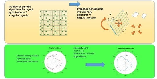
1.1.1. Contribution 1. Non-Genetic Evolutionary Algorithm Searching in a Vast Concession Area

By exploiting the complexity reduction derived from considering parallelogram-shape layout solutions (with evenly distributed turbines), this work introduces a complete WFOP that searches the optimal values for position, size and layout of the OWF in order to maximize the project profitability. Contrary to existing works based on a GA, the proposed method can search within a vast concession area without compromising the computation time. Such a complete search spectrum is only possible if the idea of using GAs to independently position each turbine is abandoned. Instead, this work proposes a non-genetic evolutionary algorithm (NGEA) that works with eight continuous variables regarding the centre coordinates, number of rows, number of turbines per row, distances between rows and between turbines in a row, row orientation and parallelogram angle.

As a relative drawback, the turbine locations cannot freely be located in the OWF area and are forced to be uniformly distributed, thus reducing the spectrum of possible candidates to the optimum. However, optimizations made with and without the restriction of uniformly distributed turbines show a very small difference in the resulting net energy yield, less than 1% [4,16,17].

1.1.2. Contribution 2. Analysis of the Optimal Orientation for Rows and Columns

The proposed method has been tested in the popular HR-I site (see Figure 1). This OWF has been used in many research works as a testing bench to prove the validity of a proposed optimization algorithm, or as a method to evaluate the wake losses. For the first objective, the output of most of the tested algorithms was a layout with turbines irregularly distributed along the concession area, and hence no useful information resulted about the preferential directions of the turbine alignments.

However, few research papers have been found discussing whether the choice of orientation and inclination of the concession area was appropriate. Gerdes in [20] stated that the turbine spacing was chosen as 560 m both between rows and along a row (equivalent to seven rotor diameter of the upwind turbine (D)), based on a wide wind direction distribution that revealed no clear preferable orientation and demanded an equal-distance spacing for both wind farm axes. The report [21] exposed that the modeled wake losses varied by only 0.11% over the full range of grid rotation, which was relatively unimportant in determining the total plant losses.

The present work analyzes the optimal values for orientation and inclination for a parallelogram-shaped OWF and compares the result to the actual layout. An additional advantage of using uniformly distributed turbines is that two of the variables defining the optimum, orientation, and inclination provides the designer with information about the preferred directions to align the turbines with the aim of being used in future for the selection of the concession area that is most attractive to developers. If the concession area is large enough, albeit with limitations in the number of turbines or MW to be installed, the algorithm also finds the optimal solution by completely defining its location, distance, orientation, inclination and layout (distribution in rows and columns).

1.2. Wake Loss Model

Regarding the models used for the evaluation of the energy produced, Archer et al. in [22] reviews and compares six popular analytical wake loss models. Among them, the vast majority of published works use the Jensen model [23] (also named as the PARK model) to calculate the wake effect at distances in excess of three turbine [24] diameters. This is the analytical model used in commercial software packages such as WAsP, WindPro and Meteodyn to evaluate the production of wind farms. In addition to the analytical models, there are others based on computational fluid dynamics (CFD) that allow a more accurate assessment of the effect of wakes. Walker et al. in [25] benchmarks the performance of four commonly used wake models against production data from five offshore wind farms. Nevertheless, the very high computational cost required makes their applicability to the optimal wind turbine micro-siting problem unfeasible in practical terms.

On the other hand, due to unavailability of the complete wind series or difficulty in their treatment, wind roses or Weibull parameters distributed in few sectors are generally used. The consideration of a discrete wind rose leads to the fact that the wake effect for incoming wind directions close to the transition zone between two sectors is not properly evaluated, which in turn causes discontinuities and unrealistic estimates of the produced energy. This aspect is even more important in the case of large offshore wind farms based on parallelogram-shaped layouts, since the errors made by concentrating all the probability on the bisector of a wind rose sector are amplified due to the high degree of symmetry, being successively reproduced for all the rows or columns.

Contribution 3. Continuous Interpolation of Sectorized Wind Data

For this reason, it is necessary to transform a sectorized wind rose into a continuous probability distribution, and analogously for the Weibull parameters. In the reviewed examples [26], the estimated distribution matches the available wind rose fairly well. However, instead of looking for a high match, a more realistic distribution will be estimated that yields the same mean value or the same cumulative probability at each sector.

To sum up, the literature review shows the existence of two gaps in the current body of knowledge on the problem of optimal micro-siting of OWFs. On the one hand, there are no previous works published that deal efficiently with the problem of optimal micro-siting of offshore wind farms based on parallelogram-shape layout, which is also one of the most common types of configurations. On the other hand, all previous works on optimal wind farm design have considered a discrete wind rose (usually composed of 8, 12 or 16 sectors), which can lead to errors in the evaluation of the wake effect with respect to a realistic situation in which the wind direction has a continuous evolution. Therefore, the present work introduces two significant improvements by developing an efficient optimization approach for parallelogram-shaped offshore wind farm designs and by introducing a new realistic model for evaluating the energy produced based on the continuous evolution of the wind resource.

The remaining of the paper is structured as follows:

• Section 2 lists the expressions for two of the most popular economic indicators used to assess the profitability of a investment, presents a brief but complete description of the Park model to evaluate the wind speed deficit, introduces a new method to interpolate a continuous distribution of the wind rose and the Weibull parameters when data for a reduced number of sectors are given, and presents the basis of the NGEA used to solve the WFOP.
• Section 3 presents and discusses the results obtained after testing it in the HR-I site;
• Finally last Section exposes the conclusions extracted from the work.

2. Materials and Methods

2.1. Economic Indicators

Rodrigues in [27] explains different economic functions to evaluate the profitability of a prospective investment over time. Among them, the levelized cost of energy (LCOE), the internal rate of return (IRR), the discounted payback time, the return on investment, or the benefit to cost ratio are used as measurements of the operation risk and the investment quality. On the other hand, the net present value (NPV) is suitable to choose between mutually exclusive options for OWF layouts and hence should be used as objective function in optimization algorithms, although limiting the maximum investment to a certain value.

Since NPV is the difference between the present value of a company’s cash inflows and the present value of cash outflows over a given time period, it can be expressed as:

$$\mathrm{NPV}=\sum _{k=1}^T\frac{AEP{p}_{kWh}{(1+\Delta p_{kWh})}^{k-1}-OPEX{(1+\Delta OPEX)}^{k-1}}{{(1+r)}^k}-CAPEX-D_{ec}$$

(1)

where T is the utility life-time, AEP is the annual net energy production (after discounting the total losses due to wake interferences and in the electrical infrastructure), p_kwh and $\Delta p_{kWh}$ are the energy price and its annual increment, OPEX and $\Delta OPEX$ are the operation and maintenance cost and its increment, CAPEX is the total investment cost and D_ec is the on-time decommissioning cost after deducing the residual price of the plant. Finally, r is the discount rate, obtained from the nominal interest rate r_i and the inflation inf as

$$r=\frac{1+r_i}{1+inf}-1.$$

(2)

The annuity factor (a) can be defined as

$$a=\sum _{k=1}^T\frac{1}{{(1+r)}^k}=\frac{1-\frac{1}{{(1+r)}^T}}{r}$$

(3)

and LCOE can be expressed as

$$\mathrm{LCOE}=\frac{CAPEX/a+OPEX}{AEP}.$$

(4)

In some research works, the discount rate is assumed to be similar to the weighted average cost of capital (WACC) and slightly higher to adjust for risk. WACC is more difficult to obtain [28], although reference values are given in [29] for Denmark, oscillating between 7.4% in 2001 and 8.9% in 2013. In this work, r_i = 9.4% and inf = 1.5% have been used, yielding r = 7.78%.

The main drawbacks of NPV are:

• A positive value is indicative of a profitable investment but does not give an idea of its quality since, in general, NPV will increase with the OWF size. It cannot be used to compare two OWFs with different sizes, locations or bid prices.
• The value of LCOE is strongly influenced by the discount rate, while the value of IRR is influenced by the sale price of the energy produced. The calculation of NPV is determined by both data, and the variation in one of them will not only produce an erroneous value in the objective function but will also distort the selection between individuals. For example, if a too low energy price or a too high discount rate have been taken, then the best solution found will tend to reduce the distances between turbines more than what is ideal.

A value of 58 €/MWh can be assigned to the energy price, as the sum of the feed-in tariff and the market price (at least during 10 years) [20,30]. Nevertheless, with this energy price, profitability is doubtful. As a consequence, LCOE has been chosen instead of NPV or IRR as a objective function, since this indicator does not depend on the energy price.

2.2. Annual Energy Production (AEP)

The annual energy produced by a wind power plant can be obtained by adding together the energy, $E_k$, produced by each of the $N_t$ turbines, for every wind direction $\phi$ and for every wind speed u. Throughout a year ($T_y=8766h$), AEP can be expressed as:

$$AEP=\sum _{k=1}^{N_t}{E}_k=T_y\sum _{k=1}^{N_t}{\int }_{u_{cut-in}}^{u_{cut-out}}{\int }_0^{2\pi }{P}_c\left({\nu }_k\right)fr(\phi ,u)\mathrm{d}u\mathrm{d}\phi$$

(5)

where $u_{cut-in}$ is the cut-in speed, $u_{cut-out}$ is the cut-out speed, $P_c$ is the electrical energy at a certain wind speed given by the turbine power curve and $fr(\phi ,u)$ is the density of probability at speed $\nu$ and wind direction $\phi$. In this expression, the power produced by a turbine k of the array depends of the effective speed of the air flow that reaches the k-th turbine, ${\nu }_k$. Due to the wake effect, this effective speed is smaller than the free-flow air speed u. There are different methods to estimate the wind speed deficit caused by the wakes.

The simplest and most popular wake model used by researchers in WFOP is the PARK model [31]. It was first proposed by Jensen and Katic [23], and starting from a diameter of the wake ($D_w$) equal to the rotor diameter of the upwind turbine (D), it assumed a expansion of the wake behind the upwind wind turbine linear with the projection of the distance between turbines onto the wind direction (s) (see Figure 2)

$$D_w=D+2k_{w}s$$

(6)

The proportionality factor is the wake decay constant (k_w), which can be expressed as a function of the tower hub height (h) and the surface roughness length (z₀)

$$k_w=\frac{0.5}{ln\left(h\right)-ln\left(z_0\right)}.$$

(7)

For the first evaluations, a value of 0.0525 was used, obtained from $z_0=0.005$ (as usual for offshore sites) and $h=70$. However, the resulting park efficiency for the HR-I layout yielded 91.5%, higher than the observed one (89% in [32]). In fact, the value obtained from (7) should be adjusted to take into account the turbulence intensity $TI$, considering that the lower the stability, the higher the $k_w$ [33]. When $TI$ is not available, authors fit $k_w$ so that the results obtained from the wake loss model match the observed values, or more frequently, they use $k_w=0.04$ for offshore sites [34]. This is the value used in this work.

According to the momentum theory, the wake expansion produces a wind speed deficit δ that depends on the upwind thurst coefficient (C_t) through

$$\delta \left(s\right)=\frac{v_{\infty }-v}{v_{\infty }}=\left(1-\sqrt{1-C_t}\right){\left(\frac{D}{D_w}\right)}^2$$

(8)

where v is the wake velocity at the downstream position and $v_{\infty }$ is the undisturbed wind speed.

In the case of turbines that are perturbed by more than one upwind turbines, the effect of the wakes must be added to obtain the effective wind speed deficit. Different methods of aggregation have been suggested [31], and among them, the preferred one is the root sum of squares

$${\delta }_{agg}^2=\sum _{i=1}^N{\delta }_i^2$$

(9)

which obtains the total wind speed deficit at any turbine as the root mean square of the deficits at downstream place due to the single wake from the N upstream turbines. In the work of Tian et al. [35], this combination method is the one that exhibits the best match with the observed power data.

The previous expression can be easily modified to account for the situation in which the downwind turbine is only partially affected by the wake. Figure 2 illustrates this situation that allows the calculation of the effective surface of the downwind rotor affected by the upstream weak (A_eff) once the projection s and the transversal separation between turbines (y) are known.

$$A^{eff}=\left\{\begin{array}{ccc}0\hfill & \mathrm{if}\hfill & y>R_w+R_t\hfill \\ \pi R_t^2\hfill & \mathrm{if}\hfill & y<R_w-R_t\hfill \\ R_w^2\left({\gamma }_w-\frac{sin\left(2{\gamma }_w\right)}{2}\right)+R_t^2\left({\gamma }_t-\frac{sin\left(2{\gamma }_t\right)}{2}\right)\hfill & \multicolumn{2}{c}{\mathrm{otherwise}}\end{array}\right.$$

(10)

with

$$\begin{array}{c}{\gamma }_w={cos}^{-1}\left(\frac{R_w^2-R_t^2+y^2}{2y{R}_w}\right)\hfill \\ {\gamma }_t={cos}^{-1}\left(\frac{R_t^2-R_w^2+y^2}{2y{R}_t}\right)\hfill \end{array}$$

(11)

and expression (9) for the wind speed deficit turns into

$${\delta }_{agg}^2=\sum _{i=1}^N{\delta }_i^2{A}_i^{eff}$$

(12)

where $A_i^{eff}$ is the surface of the partial wake of the upwind turbine i affecting the downwind turbine under study.

2.3. Continuous Distribution of Magnitudes Given by the Wind Rose and Averaged Values

Inspecting (5) makes it clear that accurate data for the density of probability $fr(u,\phi )$ are mandatory for an adequate AEP evaluation. Complete wind data sets are frequently unavailable to researchers or for a first site assessment. It is more common to have such data as values collected and summarized in a wind rose or as a set of mean values for each of the ns sectors under study.

In the case of HR-I, several sources can be found with different values, although they share the existence of a prevailing wind coming from NW. This work will use the ones obtained from [36], represented in

Table 1. Values for probability, and Weibull parameters (scale factor A at 62 m and shape factor K) for every sector.

Sector	N	NNE	NEE	E	EES	ESS	S	SSW	SWW	W	WWN	WNN
freq (%)	3.8	4.3	5.5	8.3	8.7	6.7	8.4	10.5	11.4	12.2	13.9	6.1
$Wei{b}_A$ (m/s)	8.71	9.36	9.29	10.27	10.89	10.49	10.94	11.23	11.93	11.94	12.17	10.31
$Wei{b}_K$	2.08	2.22	2.41	2.37	2.51	2.75	2.61	2.51	2.33	2.35	2.58	2.01

, resulting in the wind rose of Figure 3.

It is necessary to adjust the scale parameter A from the measurement height ($z_{ref}=62$ m) to the hub height ($z_{hub}=70$ m) due to the wind shear effect. The relationship between scale factors, and in general between wind speeds, at different heights is given by

$$A=A_{ref}\frac{ln\left(z_{hub}\right)-ln\left(z_0\right)}{ln\left(z_{ref}\right)-ln\left(z_0\right)}$$

(13)

As previously mentioned, the usual value of z₀ for offshore sites is 0.005, which is also consistent with the wind profiles presented in [36].

Logically, these data do not present a continuous evolution, and in general there appear abrupt changes in the edge from one sector to another. This unrealistic distribution prevents a proper evaluation of produced energy, leading to inconsistent situations and solutions that are far from the real one. It is therefore necessary to obtain a distribution that, although estimated, is more realistic and consistent with the continuous distributions of parameters and probabilities that are assumed for the site. Feng [26] proposed a way to obtain a continuous distribution starting from cubic spline interpolations. The result effectively describes an evolution that passes through the bisectors of the $ns$ sectors, but in general it will give rise to distributions that do not have the same mean value (in the case of the Weibull parameters), or the same cumulative probability (in the case of the wind rose) as the starting data.

Instead, this article proposes a way to obtain a continuous distribution from the averaged data for the different sectors, while respecting the aforementioned concerns. In the following, we will assume that the average value for a certain magnitude x is available for the ns sectors. At the end of this section, we will recover the Weibull parameters as this magnitude. For simplicity, we define a sector $s_i$ as

$${\mathrm{s}}_i=\left[\left.\frac{2\pi }{ns}(i-1),\frac{2\pi }{ns}i\right)\right.$$

(14)

although the explanation can be easily extended to ${\mathrm{s}}_i=\left[\left.\frac{2\pi }{ns}(i-1.5),\frac{2\pi }{ns}(i-0.5)\right)\right.$ in order to centre the first sector at the origin (0 deg). The average value for a sector i can be expressed as:

$$\overline{x_j}=\frac{ns}{2\pi }{\int }_{\frac{2\pi }{ns}(j-1)}^{\frac{2\pi }{ns}j}x\mathrm{d}\phi j\in \mathbb{N},j\le ns$$

(15)

where x can be considered as unavailable and hence unknown.

Let us define the uniform knot vector, and a vector of $ns+1$ ordinates

$$\begin{array}{cc}\hfill \mathbf{t}\hspace{1em}:=\hspace{1em}& \left\{0,t_1,\dots ,t_{ns}\right\}\mathrm{with}{t}_i=i\frac{2\pi }{ns}i\in \{0,1,\dots ns\}\hfill \end{array}$$

(16)

$$\begin{array}{cc}\hfill \mathbf{y}\hspace{1em}:=\hspace{1em}& \left\{0,y_1,\dots ,y_{ns}\right\}\mathrm{with}{y}_i=\frac{2\pi }{ns}\sum _{j=0}^i\overline{x_j}\hfill \end{array}$$

(17)

where for convenience, we can consider or define ${\overline{y}}_0={\overline{x}}_0:=0$.

A cubic spline $S\left(\phi \right)$ can be obtained as a piecewise function defined from a series of polynomials

$$P_i:[t_i,t_{i+1})\to \mathbb{R}$$

(18)

passing through the $ns+1$ points $(t_i,y_i)$, i.e., satisfying

$$S\left(t_i\right)=S\left(i\frac{2\pi }{ns}\right)=\frac{2\pi }{ns}\sum _{j=0}^i\overline{x_j}$$

(19)

On the other hand, since $S\left(t\right)$ is a cubic (i.e., smooth) spline, its derivative exits, is finite and continuous $\forall \phi \in [0,2\pi ]$. By calling

$$\tilde{x}\left(\phi \right)\frac{\mathrm{d}S\left(\phi \right)}{\mathrm{d}\phi }$$

(20)

it yields that, along a sector i, the mean value for $\tilde{x}$ is

$$\overline{\widetilde{x_i}}=\frac{ns}{2\pi }{\int }_{\frac{2\pi }{ns}(i-1)}^{\frac{2\pi }{ns}i}\widetilde{x_i}\mathrm{d}\phi =\frac{ns}{2\pi }\left(S\left(t_i\right)-S\left(t_{i-1}\right)\right)=\sum _{j=0}^i\overline{x_j}-\sum _{j=0}^{i-1}\overline{x_j}=\overline{x_i}$$

(21)

with the result that that $\tilde{x}$ is a coherent estimation of the unknown x.

Consequently, for a certain magnitude x, by finding the derivative of the cubic spline of the sum of its average values, it is possible to obtain a continuous distribution of this magnitude while keeping its mean along a sector. The procedure is:

• Calculate the accumulated sum of the average values from (16).
• Obtain the cubic spline S satisfying (19).
• An estimation of x can be found as the derivative of S.

This procedure can be applied to Weibull parameters, starting from their mean values for each of the sectors. Figure 4 shows the original discrete values for the Weibull parameters, together with their obtained continuous distributions.

The case of the wind rose is conceptually different, because the available data are the probability $P{S}_i$ that the wind comes from sector i, and the goal is to obtain a continuous distribution with the same accumulated probability at the end of each sector. However, the procedure is analogous, with the only difference of defining $y_i$ as

$$y_i:=\sum _{j=0}^{i}P{S}_i$$

(22)

with

$$P{S}_i:={\int }_{\frac{2\pi }{ns}(i-1)}^{\frac{2\pi }{ns}}p\left(\phi \right)\mathrm{d}\phi i\in \{1,2,\dots ,ns\}$$

(23)

where $p\left(\phi \right)$ is the probability density that the wind blows in the direction $\phi$ and $P{S}_i$ is the probability that the wind comes from sector i, defined by the wind rose. The estimated probability density $\tilde{p}$ is the derivative of the cubic spline, and satisfies that its aggregated value along sector i is

$$\overline{\widetilde{p_i}}={\int }_{\frac{2\pi }{ns}(i-1)}^{\frac{2\pi }{ns}i}\widetilde{p_i}\mathrm{d}\phi =\left(S\left(t_i\right)-S\left(t_{i+1}\right)\right)=\sum _{j=0}^{i}P{S}_j-\sum _{j=0}^{i-1}P{S}_j=P{S}_i$$

(24)

Therefore, $\tilde{p}$ is a coherent estimation for the probability density.

The procedure in the case of calculating a continuous probability distribution of the wind speed is:

• Obtain $P{S}_i$ from the wind rose.
• Calculate the accumulated sum of the probabilities along the sectors from (22).
• Obtain the cubic spline S.
• An estimation of p can be found as the derivative of S.

With this procedure, a continuous distribution is obtained in the interval $(0,2\pi )$ as shown in the central plot of Figure 5. However, a traditional spline interpolation does not take into account that $p\left(0\right)=p\left(2\pi \right)$. To fix this, the procedure has been repeated $ns=12$ times, exploiting the periodicity and starting the interpolation at different angles ($0,30deg,60deg\dots ,330deg$). Then, the results have been averaged to give rise to the final distribution plotted at the right of Figure 5.

2.4. Description of the Non-Genetic Evolutionary Algorithm

The aim of the WFOP is to obtain the optimal position and layout for an OWF in the concession area, such that it optimizes a certain objective function, which in this work is the LCOE. Unlike almost all of the articles reviewed, it does not seek to position each of the turbines independently [5,6,7,9,10,11,12,14,26,27], which would lead to irregular layouts. Instead, in this work, the individuals of each generation are parallelogram-shaped OWFs in which the turbines are evenly distributed. It is defined by the following 8-tuple: coordinates X and Y of the centre; number of rows (n_r); number of turbines per row (n_tr); distance between rows, in diameters (d_r); distance between turbines in a row, in diameters (d_tr); orientation of an array with respect to North, in deg, sense CW (θ); parallelogram angle; equal to 90 deg for rectangle (ϕ). Figure 6 represents these decision variables.

$$(X_c,Y_c,n_r,n_{tr},d_r,d_{tr},\theta ,\varphi ).$$

(25)

Therefore, the proposed non-genetic evolutionary algorithm (NGEA) must obtain these eight decision variables defining the OWF that minimizes the LCOE. Among them, six are real numbers and two (number of rows and columns) are discrete values. These two variables do not add additional complication because they can easily be converted to continuous values. Thus, the algorithm can be considered to work with continuous values.

In general, the following limitations apply to the presented algorithm:

• All of the turbines are of the same type and the rotors are at the same height. Therefore, it is only valid for offshore sites.
• Turbines are uniformly distributed forming a parallelogram-shaped OWF. All of the rows have the same number of turbines.
• The cable size and the substation position are optimized, but not the connection between turbines; i.e, all of the turbines of a row must be connected from the last one to the first one following a radial cable arrangement as in HR-I [37].
• The HV cable trajectory from the offshore substation to the coast transition is not optimized.

For this particular case of study, the following constraints apply:

• A maximum of 80 turbines are allowed.
• The turbine positions are limited to the shallow waters plotted in clear blue in Figure 1 (Note: the shallow waters at the right of the dashed line is considered as forbidden zone and hence disregarded). The search area in this study is limited to a reduced space, but in general the search area can be enlarged to thousands of km², without compromising the computation time.
• For the first optimization, distances between turbines in a row d_tr, and between rows d_r are fixed and equal to 7 D. For the second optimization $d_r,d_{tr}\in [5D,20D]$.

A GA like the one used by most authors working on WFOP is not appropriate for handling continuous variables. In this sense, an NGEA operating with real values has been programmed to determine the eight decision variables that define the optimal parallelogram-shaped OWF. It has basically the same structure as a typical GA, although adapting its crossover and mutation operators to work with continuous variables. The algorithm has been programmed following the operation sequence of Figure 7, where the term crossover is substituted by recombination, as usually preferred in NGEA to design the operator that combines the parents’ genotype to generate new offspring. Its operative specifications are: size of the population, 150; maximum number of generations, 250; repetitions to finish, 40; individuals in the initial population, 100; crossing probability, 80%; mutation probability, 12%.

3. Optimization Results

3.1. Anticipation of the Optimal Orientation and Inclination Angle

Before launching the algorithm that performs a complete search for the optimal solution in terms of location, dimensions and layout, an exhaustive scan has been carried out to determine the optimal orientation and inclination for a given number of turbines and separation between them. This task is not mandatory, but it will provide the designer with certain hints about the validity of the complete algorithm solutions.

The objective is to obtain the energy lost due to the wake effect, assuming the following conditions:

• The wind rose and the Weibull parameters are those specified for the HR-I site during the period 1999–2002, obtained from [36] and reproduced in Table 1. Data have been interpolated according to the method explained in Section 2.3 to estimate a continuous distribution of the density of probability and Weibull parameters.
• The number of rows and turbines per row are $n_r=10$ and $n_{tr}=8$, respectively.
• The separation between turbines of a row as well as between rows is $d_r=d_{tr}=7$ D.
• The turbines are Vestas V80, 70 m high tower. Power and thrust data were obtained from [38,39] and are shown in

  Table 2. Power and Thrust curve for Vestas V80.

  Wind Speed (m/s)	1	2	3	4	5	6	7	8	9	10	11	12	13
  Power (kW)	0	0	0	66	154	282	460	696	996	1341	1661	1866	1958
  Thrust coef	0	0	0	0.818	0.806	0.804	0.81	0.81	0.807	0.793	0.739	0.709	0.409
  Wind speed (m/s)	14	15	16	17	18	19	20	21	22	23	24	25
  Power (kW)	1988	1997	1999	2000	2000	2000	2000	2000	2000	2000	2000	2000
  Thrust coef	0.314	0.249	0.202	0.17	0.14	0.119	0.102	0.088	0.077	0.067	0.06	0.05

  .

Under these conditions, the energy deficit caused by the wake effect has been calculated for each of the possible orientations of the arrays between 0 and 180 deg, as well as for different angles of the parallelogram, between 45 and 135 deg, both with a discretization of 1 deg. The resulting AEP is shown in Figure 8. Maximum values of the produced energy are obtained for an orientation of $\theta =65deg$, and an inclination of $\varphi =91deg$. The actual layout orientation is considerable different, $\theta =173deg$, $\varphi =83deg$. Layouts producing 99.9% of the maximum energy yield are contoured in blue, highlighting that there is a large region of values for which the energy yield remains almost in its highest value. The right-hand plot shows the AEP dependence on θ for different values of ϕ. In fact, the maximum variation in AEP is 4 GWh, that represents 0.55% of the maximum yield, a reduction of 0.30 €/MWh in the LCOE, and an increase of 1.65 M€ in the NPV. This visualizes the importance of an adequate selection of these parameters.

As deduced from the wind rose of Figure 5, the most frequent wind directions are centered at the WWN direction, with very frequent winds coming from West, for which the actual OWF layout is very sensitive in terms of wind speed deficit. Thus, higher OWF efficiencies are reasonably expected for a layout arranged to alleviate the wake effect for these wind directions (see central layout of Figure 9).

The same evaluation was performed in other three situations, whose results are presented in Figure 10. The left-hand plot represents the results for a similar layout with half of the arrays and half of the columns ($5\times 4$). High similarity with the left-hand plot is observed, with a slight difference in the maximum location. This deviation is negligible because the zone contoured in blue (indicating 99.9% of the maximum energy) is very similar to that of the original $10\times 8$ layout, and any solution inside this contour will give rise to the highest (or almost) values for AEP.

The central plot chart shows an analogous representation for a quincunx layout (see the right-hand layout of Figure 9), in which the even rows are displaced by $d_{tr}^q/2$, where $d_{tr}^q$ is the distance between turbines (in a row) in this quincunx layout. In order to occupy the same concession area, $d_{tr}^q/2$ is obtained from the distance between turbines in a row, in diameters (d_tr), as

$$d_{tr}^q=d_{tr}\ast \frac{n_{tr}-1}{n_{tr}-0.5}=7·7/7.5.$$

(26)

Results are not better than the original parallelogram-shaped OWF, and it is not expected that using a quincunx layout will increase the energy yield if the distance between turbines is reduced according to (26).

Finally, the right-hand plot of Figure 10 corresponds to evaluations using the original sectorized data from sectors, without performing any interpolation. Although a logical similarity exists between this representation and that from Figure 8, there are significant differences in the maximum magnitude and location. Even when the actual values of the wind resources are unknown, the continuous distribution is more likely to behave as the real one, and the sectorized solution will give rise to erroneous results.

3.2. Possibility to Limit the Speed Range for the Deficit Calculation

During the evaluation of the energy deficit of the possible layout, the complete set of speeds is evaluated. Figure 11 plots the contribution of every speed and wind direction to the final produced energy, evidencing that only wind speeds between 5 m/s and 15 m/s are of consideration for the deficit evaluation. At lower wind speeds, the extracted power is reduced. At the other end, at speeds higher than 15 m/s, C_t is lower than 0.25 (see Table 2) and, from expression (8), the impact of wakes is reduced. In addition, the slope of the curve v-P is low at these high speeds, and moderate speed reductions will not provoke significant power deficits.

3.3. Results of the Layout Optimization Search

The algorithm shown in Section 2.4 was performed ten times to determine the best layout for a wind farm in the site where HR-I is.

The first five optimization searches were made with the constraint of limiting the turbines to the clear area corresponding to shallow waters (<10 m) of Figure 1, excluding the extraction areas and sensitive zones close to the coast. Results are presented in Figure 12. As can be seen, there is no dispersion in the location of the OWF centre (left-hand plot). The orientation and inclination are also fairly constant (central plot). The right-hand plot reflects that solutions with very long distances are preferred, since they reduce the wake effect (the maximum distance between turbines was limited to 20 D). However, concession areas are usually reduced to smaller zones, and developers are forced to reduce the separation between turbines.

According to this concern, distances were fixed to 7D, a new battery of five searches was performed, and the results are presented in Figure 13. Again, the center is well located in the middle of the concession area. Orientation values vary between 55 deg and 95 deg, while the parallelogram angles are between 85 and 95 deg. The right-hand plot shows the most frequent layouts and the mean of LCOE for every layout. The layout of 16 × 5 is the most frequent one, with the lower (i.e., best) values for the objective function LCOE. Some solutions exist with 10 × 8, 11 × 7 and 13 × 6, these two last ones including less turbines than allowed by the concessionary. These solutions hardly appear at the end of the search process if NPV is chosen as the objective function.

The evolution of the fitness at each generation is displayed in Figure 14, showing that the optimum is usually reached in less than 100 generations. The computation time is also presented, with an average of 2100 s per optimization search for long distances between turbines and 2700 s for normal separations.

Figure 15 represents the evolutions of the most frequent orientations for the rows and columns. The column orientation is obtained by subtracting the orientation and the inclination (see Figure 9). The preferred alignment directions are around 60 deg and 150 deg, trying to avoid the wind directions with more energy deficit (90 deg and 170 deg from Figure 11).

Finally,

Table 3. Configuration and cost breakdown for the actual layout, the optimal solution assuming 7D as d_r and d_tr, and the optimal solution.

	Actual	Optim	Optim		Actual	Optim	Optim
	Layout	$\mathit{d}=7\mathit{D}$	$\mathit{d}\in [5\mathit{D},20\mathit{D}]$		Layout ${}^1$	$\mathit{d}=7\mathit{D}{}^1$	$\mathit{d}\in [5\mathit{D},20\mathit{D}]{}^1$
dtr (D)	7	7	5.35	Turbines	154.8	154.8	154.8
dr (D)	7	7	19.98	Foundations	48.18	49.08	48.51
ntr	8	5	16	Electrical Offshore	58.04	60.04	58.04
nr	10	16	5	Electrical Onshore	15.88	15.88	15.88
θ (deg)	173	71.05	62.5	Others	16.60	16.60	16.60
ϕ (deg)	83	91.16	99.97	OPEX	14.24	14.47	14.97
AEP (GWh)	712.47	723.55	748.60	LCOE (€/MWh)	61.26	60.95	59.34
Elect. losses (GWh)	9.83	8.53	16.35	IRR	13.78%	13.99%	14.41%
Wake losses (GWh)	76.81	64.35	40.68	NPV (M€)	72.93	77.47	86.09

¹ Estimated costs.

lists the decision variables of the final optimum for both types of searches and compares them with the one of the actual HR-I OWF, together with the breakdown of estimated costs.

With regard to the actual layout for HR-I, the estimated park efficiency is 90.27% ($\frac{712.47}{712.47+76.81}$), reasonably close to the observed value (89%). Costs and prices were obtained from [40]. Starting from these, the estimated cost for the actual layout is EUR 293.5 M, which means 1.83 M EUR/MW. The real project cost, obtained from [20], was EUR 278 M.

The third column corresponds to the optimization result when distances between turbines are fixed and equal to 7D between rows, and between turbines in a row. Optimum orientations for rows and columns are different from the actual ones and similar to the central plot of Figure 9. However, the main difference lies in the number of rows, which in this case increases to 16, trying to orientate as much turbines as possible in the less frequent direction (71 deg together with 251 deg). The AEP improvement is 1.56% ($\frac{723.55-712.47}{712.47}$). Finally, the column $Optim[5D,20D]$ refers to the optimization result when distances are bounded between 5 and 20D. In this case, the solution results in the maximum distance (20D) between the five rows, and reduced distances (5.35D) between turbines in a row, which are aligned along less frequent wind directions. The AEP improvement is 5.09% ($\frac{748.60-712.47}{712.47}$).

With regard to the economic indicators, the investment cost hardly varies from one solution to another. An exception is the significant reduction in the collection MV electrical infrastructure for the $Optim7D$, due to grouping of sixteen turbines in the same row, for which the cable section can be optimized. For any of the solutions, the values for LCOE indicate that the price of the energy should be sufficiently higher than 60 EUR/MWh to make this project attractive to developers.

4. Conclusions and Discussion

There are numerous research works carried out on the energy losses suffered by the wake effect, especially relative to the HR-I OWF. Genetic algorithms also abound that obtain the layout that maximizes the return on investment, although none takes into account all of the factors that affect the profitability of the project. In addition, they give rise to configurations that are not desirable due to their lack of uniformity in the location of the turbines.

In this work the result of a complete optimization algorithm is presented:

• that takes into account all of the factors (or at least more than any other paper found) required for the economic evaluation;
• that fully defines the position, size and configuration of the optimal OWF with regularly distributed turbines and shaped like a parallelogram;
• that, alternatively, indicates what should be the orientation and inclination of the concession area to make it more attractive to potential developers of wind farms.

With the fixed electricity production feed-in tariff provided for grid connections at that moment equal to 0.058 EUR/kWh [20,30], the project is not profitable except for very low interest rates. In the case of uncertain values for the energy price, the most suitable indicator to evaluate the project profitability is the LCOE.

From the exploration of the results obtained with a wide concession area, a tendency is observed for the algorithm to search for very dispersed OWFs, with little exploitation of the available surface. If, to reduce the occupied area, the distance between turbines is limited to, for example, seven diameters (as is the case with HR-I), a solution search algorithm with regular patterns offers the optimal orientation, inclination and layout. In this case, and assuming the rows and columns configurations of (4 × 20, 5 × 16, 8 × 10, 10 × 8, 16 × 5, 20 × 4), an exhaustive search only needs $180\times 90\times 6\simeq$ 90,000 evaluations to calculate the optimal configuration, so that the use of a random search algorithm is meaningless. With regard to the orientation and inclination, results show that optimal solutions tend to avoid the more frequent wind direction given by the wind rose.

However, if the algorithm also has to find the exact location, orientation, inclination and optimal separation distances between turbines (respecting a more or less wide concession area), the number of possibilities increases to the extent of requiring an efficient algorithm that can handle these variables. Under these requirements, a traditional GA is not appropriate. Instead, an NGEA that operates with real values has been used to determine the decision variables that define a parallelogram-shaped OWF. The inspection of the results shows that other regular layouts were possible with a better site exploitation.

In order to have a confident estimation of wind resources, a novel method of interpolating the data given for a reduced number of sectors is presented. Consequently, the discontinuous values describing the wind direction probability and Weibull parameters are interpolated along 360 deg using cubic splines, with the concern of maintaining the accumulated probability (in the case of the wind rose) or the average value (in the case of the Weibull parameters) at each sector. Obtained results show significant differences between the optimal orientation values when the algorithms uses continuous distributions for the wind resources and when it uses sectorized data.

Additional contributions from this project are:

• discussion on the optimal orientation of the concession area for HR-I,
• recommendation to reduce the range of speeds to be studied when evaluating the orientation and inclination of the OWF during the optimization algorithm execution,
• possibility to deduce the optimal orientation and inclination replacing the original layout into a scaled version of the OWF, with half of the rows and half of the turbines per row,
• the evaluation of a quincunx configuration, which does not entail an increase in the energy produced, mainly if the position of the turbines must be limited to a certain concession area.

References

1. Walsh, C. Offshore wind in Europe. Refocus 2019, 3, 14–17. [Google Scholar]
2. Serrano González, J.; Burgos Payán, M.; Santos, J.M.R.; González-Longatt, F. A review and recent developments in the optimal wind-turbine micro-siting problem. Renew. Sustain. Energy Rev. 2014, 30, 133–144. [Google Scholar] [CrossRef]
3. Herbert-Acero, J.F.; Probst, O.; Réthoré, P.E.; Larsen, G.C.; Castillo-Villar, K.K. A review of methodological approaches for the design and optimization of wind farms. Energies 2014, 7, 6930–7016. [Google Scholar] [CrossRef]
4. Kirchner-Bossi, N.; Porté-Agel, F. Realistic wind farm layout optimization through genetic algorithms using a Gaussian wake model. Energies 2018, 11, 3268. [Google Scholar] [CrossRef] [Green Version]
5. Gao, X.; Yang, H.; Lin, L.; Koo, P. Wind turbine layout optimization using multi-population genetic algorithm and a case study in Hong Kong offshore. J. Wind. Eng. Ind. Aerodyn. 2015, 139, 89–99. [Google Scholar] [CrossRef]
6. Pookpunt, S.; Ongsakul, W. Design of optimal wind farm configuration using a binary particle swarm optimization at Huasai district, Southern Thailand. Energy Convers. Manag. 2016, 108, 160–180. [Google Scholar] [CrossRef]
7. Chowdhury, S.; Zhang, J.; Messac, A.; Castillo, L. Optimizing the arrangement and the selection of turbines for wind farms subject to varying wind conditions. Renew. Energy 2013, 52, 273–282. [Google Scholar] [CrossRef]
8. Hou, P.; Hu, W.; Soltani, M.; Chen, Z. Optimized Placement of Wind Turbines in Large-Scale Offshore Wind Farm Using Particle Swarm Optimization Algorithm. IEEE Trans. Sustain. Energy 2015, 6, 1272–1282. [Google Scholar] [CrossRef] [Green Version]
9. Salcedo-Sanz, S.; Gallo-Marazuela, D.; Pastor-Sanchez, A.; Carro-Calvo, L.; Portilla-Figueras, A.; Prieto, L. Offshore wind farm design with the Coral Reefs Optimization algorithm. Renew. Energy 2014, 63, 109–115. [Google Scholar] [CrossRef]
10. Feng, J.; Shen, W.Z. Solving the wind farm layout optimization problem using random search algorithm. Renew. Energy 2015, 78, 182–192. [Google Scholar] [CrossRef]
11. Mittal, P.; Kulkarni, K.; Mitra, K. A novel hybrid optimization methodology to optimize the total number and placement of wind turbines. Renew. Energy 2016, 86, 133–147. [Google Scholar] [CrossRef] [Green Version]
12. Mayo, M.; Daoud, M. Informed mutation of wind farm layouts to maximise energy harvest. Renew. Energy 2016, 89, 437–448. [Google Scholar] [CrossRef] [Green Version]
13. Neshat, M.; Alexander, B.; Sergiienko, N.Y.; Wagner, M. Optimisation of large wave farms using a multi-strategy evolutionary framework. In Proceedings of the 2020 Genetic and Evolutionary Computation Conference, Cancun, Mexico, 8–12 July 2020; pp. 1150–1158. [Google Scholar]
14. Kunakote, T.; Sabangban, N.; Kumar, S.; Tejani, G.G.; Panagant, N. Comparative Performance of Twelve Metaheuristics for Wind Farm Layout Optimisation. Arch. Comput. Methods Eng. 2021. [Google Scholar] [CrossRef]
15. Serrano González, J.; Trigo García, Á.L.; Burgos Payán, M.; Riquelme Santos, J.; González Rodríguez, Á.G. Optimal wind-turbine micro-siting of offshore wind farms: A grid-like layout approach. Appl. Energy 2017, 200, 28–38. [Google Scholar] [CrossRef]
16. Neubert, A.; Shah, A.; Schlez, W. Maximum Yield From Symmetrical Wind Farm Layouts. In Proceedings of the DEWEK 2010, Bremen, Germany, 17–18 November 2010; pp. 1–4. [Google Scholar]
17. Feng, J.; Shen, W.Z. Co-optimization of the shape, orientation and layout of offshore wind farms. J. Phys. Conf. Ser. 2020, 1618. [Google Scholar] [CrossRef]
18. Stanley, A.P.; Ning, A. Massive simplification of the wind farm layout optimization problem. Wind Energy Sci. 2019, 4, 663–676. [Google Scholar] [CrossRef] [Green Version]
19. Lv, M.; Li, J.; Du, H.; Zhu, W.; Meng, J. Solar array layout optimization for stratospheric airships using numerical method. Energy Convers. Manag. 2017, 135, 160–169. [Google Scholar] [CrossRef]
20. Gerdes, G.; Albrecht, T.; Zeelenberg, S. Case Study: European Offshore Wind Farms—A Survey for the Analysis of the Experiences and Lessons Learnt by Developers of Offshore Wind Farms; Technical Report; Deutsche WindGuard GmbH: Varel, Germany, 2005. Available online: https://tethys.pnnl.gov/publications/case-study-european-offshore-wind-farms-survey-analysis-experienceslessons-learnt (accessed on 14 May 2021).
21. Musial, W.; Parker, Z.; Fields, J.; Scott, G.; Elliott, D.; Draxl, C. Assessment of Offshore Wind Energy Leasing Areas for the BOEM Massachusetts Wind Energy Area; Technical Report October; National Renewable Energy Laboratory, 2012. Available online: https://www.nrel.gov/docs/fy14osti/60942.pdf (accessed on 14 May 2021).
22. Archer, C.L.; Vasel-Be-Hagh, A.; Yan, C.; Wu, S.; Pan, Y.; Brodie, J.F.; Maguire, A.E. Review and evaluation of wake loss models for wind energy applications. Appl. Energy 2018, 226, 1187–1207. [Google Scholar] [CrossRef]
23. Katic, I.; Højstrup, J.; Jensen, N. A Simple Model for Cluster Efficiency Publication date. In Proceedings of the European wind energy association conference and exhibition, Rome, Italy, 7–9 October 1987; Volume 1, pp. 407–410. [Google Scholar]
24. Barthelmie, R.J.; Folkerts, L.; Larsen, G.C.; Rados, K.; Pryor, S.C.; Frandsen, S.T.; Lange, B.; Schepers, G. Comparison of Wake Model Simulations with Offshore Wind Turbine Wake Profiles Measured by Sodar. J. Atmos. Ocean Technol. 2006, 23, 888–901. [Google Scholar] [CrossRef]
25. Walker, K.; Adams, N.; Gribben, B.; Gellatly, B.; Nygaard, N.G.; Henderson, A.; Marchante Jimemez, M.; Schmidt, S.R.; Rodriguez Ruiz, J.; Paredes, D.; et al. An evaluation of the predictive accuracy of wake effects models for offshore wind farms. Wind Energy 2016, 19, 979–996. [Google Scholar] [CrossRef]
26. Feng, J.; Shen, W.Z. Modelling wind for wind farm layout optimization using joint distribution of wind speed and wind direction. Energies 2015, 8, 3075–3092. [Google Scholar] [CrossRef] [Green Version]
27. Rodrigues, S.; Restrepo, C.; Katsouris, G.; Pinto, R.T.; Soleimanzadeh, M.; Bosman, P.; Bauer, P. A multi-objective optimization framework for offshorewind farm layouts and electric infrastructures. Energies 2016, 9, 216. [Google Scholar] [CrossRef] [Green Version]
28. Levitt, A.C.; Kempton, W.; Smith, A.P.; Musial, W.; Firestone, J. Pricing offshore wind power. Energy Policy 2011, 39, 6408–6421. [Google Scholar] [CrossRef]
29. Voormolen, J.A.; Junginger, H.M.; van Sark, W.G. Unravelling historical cost developments of offshore wind energy in Europe. Energy Policy 2016, 88, 435–444. [Google Scholar] [CrossRef]
30. Danish Energy Authority, Amaliegade 44 1256 Copenhagen K. Offshore Wind Power- Danish Experiences and Solutions; Technical Report; Danish Energy Authority: Amaliegade, Denmark, 2005; ISBN 87-7844-560-4. Available online: https://discomap.eea.europa.eu/map/Data/Milieu/OURCOAST_097_DK/OURCOAST_097_DK_Doc4_ExpSolutionsDK.pdf (accessed on 14 May 2021).
31. Shao, Z.; Wu, Y.; Li, L.; Han, S.; Liu, Y. Multiple wind turbine wakes modeling considering the faster wake recovery in overlapped wakes. Energies 2019, 12, 680. [Google Scholar] [CrossRef] [Green Version]
32. Sørensen, T.; Lybech, M.; Nielsen, P. Adapting and Calibration of Existing Wake Models to Meet the Conditions Inside; Technical Report 27491529; EMD International A/S: Aalborg, Denmark, 2008; Available online:https://www.emd.dk/files/PSO%20projekt%205899.pdf (accessed on 14 May 2021).
33. Hansen1, K.; Barthelmie, R.J.; Jensen, L.E.; Sommer, A. The impact of turbulence intensity and atmospheric stability on power deficits due to wind turbine wakes at Horns Rev wind farm. Wind Energy 2012, 15, 183–196. [Google Scholar] [CrossRef] [Green Version]
34. Barthelmie, R.J.; Pryor, S.C.; Frandsen, S.T.; Hansen, K.S.; Schepers, J.G.; Rados, K.; Schlez, W.; Neubert, A.; Jensen, L.E.; Neckelmann, S. Quantifying the impact of wind turbine wakes on power output at offshore wind farms. J. Atmos. Ocean Technol. 2010, 27, 1302–1317. [Google Scholar] [CrossRef]
35. Tian, L.; Zhu, W.; Shen, W.; Song, Y.; Zhao, N. Prediction of multi-wake problems using an improved Jensen wake model. Renew. Energy 2017, 102, 457–469. [Google Scholar] [CrossRef]
36. Li, S. Wind Array Performance Evaluation Model for Large Wind Farms and Wind Farm Layout Optimization. Thesis, 2014. Available online: https://etd.ohiolink.edu/apexprod/rws_etd/send_file/send?accession=case1405080318 (accessed on 14 May 2021).
37. Lingling, H.; Yang, F.; Xiaoming, G. Optimization of electrical connection scheme for large offshore wind farm with genetic algorithm. In Proceedings of the 2009 International Conference on Sustainable Power Generation and Supply, Nanjing, China, 6–7 April 2009; pp. 1–4. [Google Scholar] [CrossRef]
38. Pedersen, M.M.; van der Laan, P.; Friis-Moller, M.; Rinker, J.; Rethore, P.E. DTUWindEnergy/PyWake: PyWake. 2019. Available online: https://topfarm.pages.windenergy.dtu.dk/PyWake/ (accessed on 14 May 2021). [CrossRef]
39. Wu, Y.T.; Porte-Agel, F. Atmospheric Turbulence Effects on Wind-Turbine Wakes: An LES Study. Energies 2012, 5, 5340–5362. [Google Scholar] [CrossRef]
40. Gonzalez-Rodriguez, A.G. Review of offshore wind farm cost components. Energy Sustain. Dev. 2016. [Google Scholar] [CrossRef]
Figure 1. Nautical chart including depths, coast and forbidden zones for HR-I site.
Energies 14 02895 g001
Figure 2. Downwind turbine partially covered by an upwind stream.
Energies 14 02895 g002
Figure 3. Wind rose obtained from [36]. Only values between cut-in speed and cut-out speed are represented.
Energies 14 02895 g003
Figure 4. Original discrete values for the Weibull parameters, and their corresponding continuous distributions.
Energies 14 02895 g004
Figure 5. Continuous interpolation of a wind rose. Left: Original wind rose for twelve sectors. Center: continuous distribution with abrupt edge from NNW to N. Right: original wind rose compared to an averaged distribution.
Energies 14 02895 g005
Figure 6. Decision variables defining the candidates for the optimal OWF that maximizes the LCOE.
Energies 14 02895 g006
Figure 7. Flowchart of operations performed by the optimization algorithm.
Energies 14 02895 g007
Figure 8. Energy deficit and AEP at different orientations and inclinations. Left: contour lines for constant levels of energy deficit when a continuous estimated distribution is used. The optimal values are pointed out with red asterisks and actual values for HR-I with a circle. Zones with 99.9% of the maximum yield are contoured in blue. Right: variation of AEP with the orientation at different inclinations.
Energies 14 02895 g008
Figure 9. Aspect of a HR-I layout when modifying the orientation and inclination. Layout for the actual OWF (left-hand), for the estimated optimum (centre) and for the estimated optimum assuming a quincunx arrangement (right-hand).
Energies 14 02895 g009
Figure 10. Comparison of the energy produced in different scenarios. Contour lines for constant levels of energy deficit for a simplified 5 × 4 layout (left-hand plot), using the original discretized data (central plot) and for a quincunx layout (right-hand plot). The optimal values are pointed out with red asterisks, and zones with 99.9% of the maximum yield are contoured in blue.
Energies 14 02895 g010
Figure 11. Contribution of different wind speeds and directions to the produced power and energy. Electric power produced by the OWF for every wind speed and wind direction (left-hand plot) and energy taking into account the density of probability (right-hand plot). Contour lines are added for a value = 1% of the maximum one.
Energies 14 02895 g011
Figure 12. Parameters of the best individuals when the solution is constrained to a large concession area (in white in Figure 1). Left: center location of the best individuals at each generation. Middle: orientation angle of the rows and parallelogram angle. Right: separation between turbines in a row, and between rows. Results for the ten optimization searches are represented with different colors.
Energies 14 02895 g012
Figure 13. Parameters of the best individuals when the solution is constrained to a large concession area (in white in Figure 1) and 7 D are imposed as distances between turbines. Left: center location of the best individual at each generation. Middle: orientation angle of the rows and parallelogram angle. Results for the ten optimization searches are represented with different colors. Right: mean of the LCOE and number of occurrences for individuals having a certain number of turbines per row.
Energies 14 02895 g013
Figure 14. Evolution of the fitness and the simulation time during the search process.
Energies 14 02895 g014
Figure 15. Preferred orientations for rows (o) and columns (*) of the best individual at each generation. Results for the five optimization searches are represented with different colors. The plot at the left represents the values when no separation restriction is imposed to the separation between rows and columns. In the right-hand plot, a separation of 7D is imposed.
Energies 14 02895 g015