Article

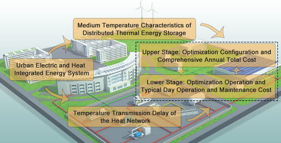
Distributed Thermal Energy Storage Configuration of an Urban Electric and Heat Integrated Energy System Considering Medium Temperature Characteristics

1
Key Laboratory of Smart Grid of Ministry of Education, Tianjin University, Tianjin 300072, China
2
State Grid Economic and Technological Research Institute Co. Ltd., Beijing 102209, China
*
Author to whom correspondence should be addressed.
Energies 2021, 14(10), 2924; https://doi.org/10.3390/en14102924
Submission received: 27 April 2021 / Revised: 14 May 2021 / Accepted: 17 May 2021 / Published: 18 May 2021

Abstract

:
Distributed thermal energy storage (DTES) provides specific opportunities to realize the sustainable and economic operation of urban electric heat integrated energy systems (UEHIES). However, the construction of the theory of the model and the configuration method of thermal storage for distributed application are still challenging. This paper analyzes the heat absorption and release process between the DTES internal heat storage medium and the heat network transfer medium, refines the relationship between heat transfer power and temperature characteristics, and establishes a water thermal energy storage and electric heater phase change thermal energy storage model, considering medium temperature characteristics. Combined with the temperature transmission delay characteristics of a heat network, a two-stage optimal configuration model of DTES for UEHIES is proposed. The results show that considering the temperature characteristics in the configuration method can accurately reflect the performance of DTES, enhance wind power utilization, improve the operation efficiency of energy equipment, and reduce the cost of the system.

Graphical Abstract

1. Introduction

In order to deal with increasingly severe energy and environmental problems, the development of renewable energy and the improvement of energy structures have become a common goal in many countries and regions [1,2]. Currently, wind power and other renewable power generation technologies are widely used in the field of renewable energy utilization [3]. However, due to the randomness and volatility of wind power, there are still some obstacles to its high usage proportion and stable consumption. The development of urban electric heat integrated energy systems (UEHIES) is an effective way to promote the utilization of large-scale renewable energy and reduce the operation and maintenance costs of energy systems, which have been a focus of scholars in recent years [4,5]. Among the various energy technologies, distributed thermal energy storage (DTES), represented by water storage [6] and phase change storage [7], has the distinguishing features of a flexible operation [8], short construction period, and low investment costs [9], which has a positive role in the further optimization of UEHIES. This method has attracted extensive attention from researchers all over the world. Reasonably configuring DTES has become an important research topic.
The DTES model is the basis of optimal configuration. In the current research into DTES configuration, the construction of DTES models mainly focuses on two aspects. The first takes the energy balance as the core constraint into account and each schedule cycle is divided into a heat absorbing period and a releasing period, based on the principle of heat balance [10,11,12]. The application of this model is mainly to improve the demand side. Storage equipment absorbs heat power at the time of valley load and then releases it at the time of peak load to realize peak load cutting and valley filling, lessening the carbon emissions of the distributed energy system [10], cutting down the heat loss of the heat network [11], and reducing the investment costs related to the equipment [12]. The second approach is analogous with the state of charge model of electric energy storage and is used to establish the thermal state model, coupling with time series and heat exchange power [13,14,15,16]. In [13], the DTES model was used to regulate the secondary heat network in distributed energy stations. Through optimal scheduling of energy storage, the flexibility of an energy station could be improved. In [14], the authors proposed that DTES could enhance the ability of active demand response. By optimizing the capacity of a thermal storage tank, the operation cost of a heat supply station could be reduced, and comfort on the demand side could be upgraded. In [15], the authors showed that there was a restrictive relationship between investments, heat load, heat price, and operational revenue, and regional retailers could maximize their benefits by configuring different equipment. In [16], the authors took the heat network of Aarhus in Denmark as the research object, established a configuration model considering the payback period of investment, and showed that DTES had a good effect on the system with a significant fluctuation in the heat sale price.
Aiming at the optimal configuration of DTES, in [17], the authors studied the operation states of heat supply devices installed in a distributed energy station during a cold winter period and proposed a configuration method using thermal energy storage to adjust the temperature fluctuations of a heat pump. The evaporation temperature of the heat pump was increased with the help of heat release at night, which improved performance in terms of the heat coefficient. In [18,19], the authors studied a distributed integrated energy microgrid, in which the wind power consumption percentage was low. Considering the investment cost of thermal energy storage and the penalty cost of wind curtailment, a configuration model was proposed to minimize the total cost. During the period of wind curtailment, most of the heat supply tasks were undertaken by electric boilers and storage devices, so the wind power consumption space was improved. From the perspective of future planning, in [20], the authors proposed a configuration method with minimum emissions in the whole life cycle, considering the growth of heat load, climate warming, and other factors. A community in Spain was taken as a case to study the impact of a DTES system with a different design life. In [21], the authors analyzed the energy efficiency and environmental protection requirements of a future energy system. The material and capacity selection method of phase change thermal storage was studied. With the help of storage equipment, the heat supply schedule of the energy system was readjusted, the utilization efficiency of primary energy was improved, and the carbon emissions were reduced. In [22], the authors focused on the power quality of a regional integrated energy system under the background of increasing wind power penetration. The heat storage capacity and installed location of electric heaters and thermal energy storage systems were studied. The voltage fluctuations could be reduced by configuring storage equipment in nodes with a high coupling degree of electricity and heat. In [23], the authors analyzed a future energy market and user demand and put forward a business model of a thermal storage cloud. By evaluating the investment costs of different DTES systems and the benefits of providing ancillary services, a cloud investor could choose the most profitable configuration scheme.
Based on the above research, the following insufficiencies faced by the optimal configuration of DTES can be summarized: firstly, in DTES models, it is generally considered that the temperature of a heat medium is constant in the process of heat absorption and release, ignoring the temperature characteristics of heat transfer, which means that the comprehensive influence of storage equipment’s internal structure, such as the heat exchange area, mass flow, and other parameters, are not reflected. This leads to a decline in model accuracy and brings about a deviation from the expected value in the design scheme. Secondly, presently, UEHIES is mostly described by power flow [18,22]. However, this method can hardly reflect the differences in all kinds of energy. As two energy forms with different energy attributes and transmission characteristics, electric and heat exhibit different actual operation performances, especially in the case of the temperature transmission delay in an urban heat network in UEHIES with long pipes and a large mass flow [24,25]. Some studies have shown that the two models, considering the temperature transmission delay characteristics and ignoring the operation schedules of heat sources, show obvious diversity [26], and the heat supply medium temperature of each node in the primary heat network is significantly different [27].
In view of the above, starting from the internal structure of DTES, this paper analyzes the heat charge and discharge performances of two typical DTES devices—water thermal energy storage (WTES) and electric heater phase change thermal energy storage (EH-PHTES)—and presents a DTES model considering medium temperature characteristics. Then, the temperature transmission delay characteristics of the heat network (TTD-HN) and the medium temperature characteristics of DTES (MTC-DTES) are introduced into the construction of a model of an urban heat network, and a two-stage optimal configuration method of DTES is proposed. The objective of the upper optimization stage is to minimize the comprehensive annual total cost of the whole system, and the layout nodes, the storage tank, and the heat exchanger capacity are selected. The objective of the lower optimization stage is to minimize the typical daily operation and maintenance costs. Combined heat and power (CHP) and thermal power generation (TPG) outputs, DTES heat charge and discharge power, and other operating parameters are taken as optimization objects. Finally, the effectiveness of the method is verified using a case study. Subsequently, the influences of different thermal storage equipment, load types, and wind power capacity on the DTES configuration are discussed and configuration schemes of distributed and centralized thermal energy storage are compared and analyzed.

2. Medium Temperature Characteristics of Distributed Thermal Energy Storage Models

In UEHIES, there may be a variety of thermal energy storage devices. According to the installation location, they can be divided into centralized and distributed. Centralized thermal energy storage is generally a large heat storage device which is installed in the heat source station. Distributed thermal energy storage aims to arrange small heat storage devices at the heat exchange station (HES), and regulate the heat power of HESs.
DTESs store heat using various heat storage mediums, absorb heat from the high temperature heat transfer medium of the primary heat network or from the electric heater equipment, and then release heat to the low temperature heat transfer medium from the secondary heat network. The temperature characteristics of the heat storage medium and heat transfer medium have an essential impact on the heat exchange process of DTES, which should not be ignored in the DTES configuration model. In this study, WTES and EH-PHTES, which are presently widely used, are taken as the specific research objects for modeling.

2.1. Water Thermal Energy Storage

WTES consists of a water tank, two heat exchangers (HEXs), and some pipes and valves. The water tank uses a natural stratification effect to store heat. The HEXs are responsible for charging heat from the primary heat network and discharging it to the secondary heat network. The storage medium in the water tank can be divided into three layers: the upper temperature zone, thermocline, and the lower temperature zone. The upper and lower temperature zones have a large thickness and a slight temperature difference in their respective regions, which can be approximately regarded as constant temperature regions and are the main effective utilization zones of energy storage. The thermocline has an obvious temperature change and small thickness and mainly plays the role of insulation and heat preservation. The HEX has a primary side and a secondary side. There is only heat exchange between the two sides and no hydraulic exchange. The high temperature medium flows in the primary side from the inlet to the outlet. The low temperature medium flows in the secondary side from the outlet to the inlet. The medium temperature zones and device connections of a WTES system are shown in Figure 1.
During the heat charging period, the high temperature medium from the primary heat network flows into the primary side of the WTES HEX; afterwards, the heat is delivered to the secondary side of WTES HEX, increasing the temperature of the WTES circulating medium and storage medium [28,29]. The distances between the inlet, outlet, HEX, and water tank are usually very close. The heat loss in the transfer process is negligible. It is assumed that the heat power released by the heat transfer medium of the primary heat network, the heat power exchanged by the HEX, and the heat power received by the water tank are basically the same.
The relationship between the heat transfer and the storage medium is based on the heat exchange theory in [28,29]. It can be described as follows:
H N E T = m N E T c f N E T ( T s N E T T r N E T )  
H H E X = K F ( Δ T d Δ T x ) ln ( Δ T d ) ln ( Δ T x )
H W T E S = m W T E S c f W T E S ( T u p p e r W T E S T l o w e r W T E S )
H N E T = H W T E S = H H E X
Equations (1)–(3) describe the calculation of the heat power released by the heat network ( H N E T ), the heat power exchanged by HEX ( H H E X ), and the heat power absorbed by the WTES water tank ( H W T E S ). Based on the previous assumptions, Equation (4) is obtained. m N E T is the mass flow of the heat network into HEX, m W T E S is the mass flow of WTES circulating pipe into HEX, T s N E T and T r N E T are the temperature of the heat network into HEX inlet and outlet, c f N E T and c f W T E S are the specific heat capacity of the heat transfer medium in the heat network and the heat storage medium in the WTES. T u p p e r W T E S and T l o w e r W T E S are the temperature of the upper and lower temperature zones, Δ T d and Δ T x is the temperature difference at the HEX inlet and outlet.
K F is the heat transfer capacity of HEX, which is obtained by multiplying the overall heat transfer coefficient and total heat exchange area [30]. The area is related to the production process and can be configured artificially. The instantaneous value of overall heat transfer coefficient of the HEX will be affected by the turbulence state and the scaling degree [30,31]; the actual value is difficult to measure. In the configuration model, the total heat exchange over a period of time (e.g., 1 h) is of more interest than the instantaneous heat power. Thus, the rated overall heat transfer coefficient is more suitable to be used for the calculation of heat transfer capacity. In this article, the designed heat transfer capacity of HEX, K F 1 W T E S , is used to replace K F , which is obtained by multiplying the rated overall heat transfer coefficient and total heat exchange area. Equation (2) can be rewritten as Equation (5) accordingly [32,33].
H H E X = K F 1 W T E S ( Δ T d Δ T x ) ln ( Δ T d ) ln ( Δ T x )
The logarithmic mean temperature difference in Equation (2) is nonlinear, which is approximated linearly under the condition that:
0.6 Δ T d Δ T x 1.7
This condition can be satisfied in most counter flow DTES scenarios. The approximation of Equation (2) can be expressed as follow [34].
H H E X = K F 1 W T E S ( Δ T d + Δ T x ) 2
At the same time, it is assumed that the temperature of the heat network transfer medium flowing into the HEX is consistent with the temperature of the HES supply pipe connected to the primary heat network ( T s , 1 H E S ). The temperature difference calculation formulas at the HEX inlet and outlet are taken from [34]. Some of the parameters in Equations (1)–(4) are shown in Equations (8)–(10).
Δ T d = T s N E T T u p p e r W T E S
Δ T x = T r N E T T l o w e r W T E S
T s N E T = T s , 1 H E S
According to Equations (1)–(4), the relationship between the WTES heat charging power and the temperature of the HES supply pipe connected to the primary heat network can be deduced; additionally, the relationship between the thermal resistance of WTES connected to the primary heat network and the mass flow of the primary heat network flowing into the HEX can also be deduced. The expression is as follows:
H i , t W T E S , C H = T s , i , t , 1 H E S T ave , i W T E S R i , t , 1 W T E S
R i , t , 1 W T E S = 1 K F i , 1 W T E S + 1 2 m i , t , 1 N E T c f N E T
where the subscript i is the node number, the subscript t is the time interval number, the subscript 1 is the connection to the primary heat network, and the subscript 2 is the connection to the secondary heat network. For example, H i , t W T E S , C H is the heat charging power of WTES in node i at time t , R i , t , 1 W T E S is the thermal resistance of WTES connected to the primary heat network in node i at time t . T ave , i W T E S is the average value of T u p p e r W T E S and T l o w e r W T E S . The following variable naming follows this rule, and the variable subscripts are no longer explained separately.
It can be seen from Equations (11) and (12) that the heat charging power is positively correlated with medium temperature; the higher the temperature of the heat transfer medium, the higher the WTES heat charging power. The thermal resistance is negatively correlated with mass flow; the larger the mass flow, the smaller the thermal resistance coefficient. At the same time, the mass flow into the heat exchanger is controlled by relevant valves and water pumps, and its maximum value cannot exceed the mass flow of primary heat network in HES ( m i , 1 H E S ).
m i , t , 1 N E T m i , 1 H E S
Similarly, the relationship between the WTES heat discharging power and the medium temperature of the HES return pipe connected to the secondary heat network, the relationship between the thermal resistance of WTES system connected to the secondary heat network and the mass flow of the secondary heat network into the HEX, are as follows:
H i , t W T E S , D I S = T ave , i W T E S T r , i , t , 2 H E S R i , t , 2 W T E S
R i , t , 2 W T E S = 1 K F i , 2 WTES + 1 2 m i , t , 2 N E T c f N E T
where H i , t W T E S , D I S is the heat discharging power of WTES and R i , t , 2 W T E S is the thermal resistance of WTES connected to the secondary heat network.
It can be seen from Equations (14) and (15) that the heat discharging power is negatively correlated with medium temperature; the lower the temperature of the heat transfer medium, the higher the WTES heat discharging power. The thermal resistance is negatively correlated with the mass flow; the larger the mass flow, the smaller the thermal resistance coefficient. At the same time, the mass flow’s maximum value cannot exceed the mass flow of primary heat network in the HES ( m i , 2 H E S ).
m i , t , 2 N E T m i , 2 H E S
In the configuration process, the configuration heat capacity ( S c a p , i W T E S ) is usually related to the volume of the container [8,20]. In this article, it indicates the heat when the water tank is full of the upper temperature medium, representing the maximum heat storage quantity in theory. In the operation process, the change of the actual energy stored in the water tank ( S i , t W T E S ) should consider the influence of the heat charging and discharging power and the balance between the energy change of two adjacent time intervals according to [14]. At the same time, due to the influence of factors such as the thickness of thermocline, the internal energy has the following maximum and minimum constraints by referring to [13,15].
S c a p , i W T E S = ρ i W T E S V i W T E S c f , i W T E S ( T u p p e r , i W T E S T l o w e r , i W T E S )
S i , t + 1 W T E S = S i , t W T E S H i , t W T E S , D I S Δ t + H i , t W T E S , C H Δ t
S i , m i n W T E S S i , t W T E S S i , m a x W T E S
where ρ i W T E S is the density of WTES heat storage medium, V i W T E S is the internal volume of WTES water tank, Δ t is the time interval, S i , m a x W T E S and S i , m i n W T E S is the maximum and minimum constraint values of the actual energy stored in the water tank.
In addition, in order to keep the flow and pressure stable, the WTES heat charging and heat discharging power cannot be carried out at the same time.
H i , t W T E S , C H H i , t W T E S , D I S = 0

2.2. Electric Heater Phase Change Thermal Energy Storage

EH-PHTES is composed of an electric heater (EH), a phase change tank, and a HEX. EH directly generates heat using energy conversion technology. The phase change material is placed in the phase change tank to store heat in the form of latent heat. The phase change material in the tank is in the state of solidification and melting coexistence. Heating electrodes and some circulating pipes are arranged in the phase change tank. Heating electrodes can release heat to phase change materials to make them melted. After some time, with the increase of melting material, the proportion of solidification and melting reaches a new balance point. The circulating pipes contain a heat circulating medium, which can absorb heat from phase change materials and release them to the HEX. Similarly, with the increase of solidification material, the proportion of solidification and melting reaches another new balance point.
There is a great deal of research to reduce the time spent in the process of heat transfer [35,36]. The thermal energy storage in distributed application scenarios can completely store or release heat in several minutes [37]. In the configuration model, it can be approximately considered that the material in EH-PHTES of each operation interval has reached balance points.
The internal structure of EH-PHTES and the device connections are shown in Figure 2.
The choice of phase change materials should have a reasonable phase change temperature. In the HES, the phase change temperature is generally required to be in the range of 50–90 °C. In addition, phase change materials are required to have enough generality. Typical phase change materials include organic materials represented by paraffin, fatty acids, alcohols, and esters, and inorganic materials represented by hydrated salts [8].
In the process of heat charging, EH-PHTES does not exchange heat through the HEX but rather through the EH. The relationship between the heat charging power ( H i , t E H - P H T E S , C H ) and the electric power ( P i , t E H ) of the EH can be expressed by the electric to thermal efficiency of EH η i E H according to [38], which represents the ratio of the unit thermal power generated by EH to the electric power consumed.
H i , t E H - P H T E S , C H = P i , t E H η i E H
P i , t E H P R a t e d , i E H
According to [38,39], in a well-maintained system, the efficiency is close to 100%. The electric power shall not exceed the rated power ( P R a t e d , i E H ).
During the heat discharging process, the medium temperature characteristics of the phase change tank are different from those of the water tank. When the phase change material changes between the solid and the liquid, the phase change temperature is constant, and the relationship between the phase change temperature and the heat discharging power can be expressed as follows:
H E H - P H T E S = m P H T E S c f P H T E S ( T P H T E S T r P H T E S )
In Equation (23), the heat discharging power of EH-PHTES ( H E H - P H T E S ) is related to the phase change temperature ( T P H T E S ), return temperature ( T r P H T E S ), internal circulation medium mass flow ( m P H T E S ), and specific heat capacity ( c f P H T E S ).
Equations (1), (2) and (4) can still be used to describe the process of heat transfer from the HEX’s primary side to the secondary heat network. However, the setting of each parameter is different. K F 2 E H P H T E S is chosen to replace K F in Equation (2). At the same time, it is assumed that the heat network medium temperature flowing into the HEX is consistent with the temperature of the HES return pipe connected to the secondary heat network.
H H E X = K F 2 E H - P H T E S ( Δ T d + Δ T x ) 2
Δ T d = T P H T E S T s N E T
Δ T x = T r P H T E S - T r N E T
T r N E T = T r , 2 H E S
According to the heat transfer process of Equations (1), (4), (23) and (24), the relationship between the EH-PHTES heat discharging power and the temperature of the HES return pipe connected to the secondary heat network, and the relationship between the EH-PHTES heat discharging resistance coefficient and the mass flow of the secondary heat network into HEX, are as follows:
H i , t E H - P H T E S , D I S = T i P H T E S T r , i , t , 2 H E S R i , t , 2 E H - P H T E S
R i , t , 2 E H - P H T E S = 1 K F i , 2 E H - P H T E S + 1 2 m i , t , 2 N E T c f N E T + 1 2 m i P H T E S c f P H T E S
where H i , t E H - P H T E S , D I S is the heat discharging power of EH-PHTES, R i , t , 2 E H - P H T E S is the thermal resistance of EH-PHTES connected to the secondary heat network.
It can be seen from Equations (28) and (29) that the heat discharging power is negatively correlated with medium temperature; the lower the temperature of the heat transfer medium, the higher the EH-PTES heat discharging power. The thermal resistance is negatively correlated with the mass flow; the larger the mass flow, the smaller the thermal resistance coefficient. At the same time, the mass flow maximum value cannot exceed the mass flow of primary heat network in the HES.
m i , t , 2 N E T m i , 2 H E S
In the configuration process, the configuration heat capacity ( S c a p , i P H T E S ) is related to the volume of the container. In this article, it indicates the heat when the phase change tank is full of the liquid phase material, in theory representing the maximum heat quantity. In the operation process, the change of the actual energy stored in the phase change tank ( S i , t P H T E S ) should consider the influence of the heat charging and discharging power, and the balance between the heat change of two adjacent time intervals. At the same time, the internal energy has the following maximum and minimum requirements:
S c a p , i P H T E S = ρ i E H - P H T E S V i E H - P H T E S L f , i E H - P H T E S
S i , t + 1 P H T E S = S i , t P H T E S + H i , t E H - P H T E S , C H Δ t H i , t E H - P H T E S , D I S Δ t
S i , m i n P H T E S S i , t P H T E S S i , m a x P H T E S
where ρ i E H P H T E S is the density of EH-PHTES heat storage medium, V i E H P H T E S is the internal volume of EH-PHTES container, L f , i E H - P H T E S is the latent heat of EH-PHTES, S i , m a x P H T E S and S i , m i n P H T E S is the maximum and minimum constraint value of the actual energy stored in EH-PHTES.
EH-PHTES is only connected with the secondary heat network in the urban heat network and has no physical connection with the primary heat network. Thus, EH-PHTES can charge from the EH and discharge to the secondary heating network simultaneously.

3. Urban Electric and Heat Integrated Energy System Models

The UEHIES is mainly composed of electric and heat production equipment, electric heat coupling devices, an urban electric power grid and an urban heat network. A typical urban electric thermal integrated energy system is shown in Figure 3.
The electric heat coupling devices contain the interaction of electricity and heat, which is the main link between energy production and conversion. The urban electric power grid and heat network connect the energy coupling links, which is the key to realizing the balance of voltage, temperature, and energy in the system. In order to focus on the research points, the independent heat production equipment is not modeled nor analyzed in this paper.

3.1. Electric Heat Coupling Device

In the UEHIES, the CHP unit is the most common electric heat coupling device. In the operational area of cogeneration, electric power ( P C H P ) and thermal power ( H C H P ) are interdependent [40,41]. Any operation point in this polygonal operation area can be represented by the combination of corner coordinates by the combination coefficient.
H C H P = k Γ k ( α k H k C H P )
P C H P = k Γ k ( α k P k C H P )
0 α k 1
k = 1 N α k = 1
where Γ k is the set of numbers of corner coordinates and α k is the combination coefficient of corner coordinate k in the CHP polygonal operation area. H k C H P and P k C H P are the heat and electric power of corner coordinate k in the CHP polygonal operation area.
The ramping constraint of the CHP is shown in Equation (38):
Δ P R a m p C H P P t C H P P t + 1 C H P Δ P R a m p C H P
where Δ P R a m p C H P is the ramp power of CHP.

3.2. Wind Power

From the relationship between wind speed ( v i , t ) and wind power generation, the predicted wind power of wind farm ( P i , t W , p r e ) can be obtained according to [42,43]:
P i , t W , p r e = { 0 v i , t < v i c u t - i n   o r   v i , t > v i c u t - o u t v i , t v i c u t - i n v i r a t e d v i c u t - i n P r W v i r a t e d v i , t v i c u t - i n   P i , r W v i c u t - o u t v i , t v i r a t e d
where v i c u t - i n and v i c u t - o u t is the cut in and cut out wind speed of wind power generation, P i , r W is the rated wind power of wind power generation, and v i r a t e d is the rated wind speed of wind power generation.
In actual operation, the electric power grid may not be able to accept all the wind power, and wind curtailment may occur. The wind curtailment power ( P i , t W , c u r ) is the difference between predicted wind power and real wind power ( P i , t W , r e a l ).
P i , t W , r e a l P i , t W , p r e
P i , t W , c u r = P i , t W , p r e P i , t W , r e a l

3.3. Power Plant

The levelized cost of energy (LCOE) method is commonly used to estimate the fuel consumption of various TPGs [44,45,46]. Fuel consumption ( F i , t T P G ) is related to the electric power of TPG ( P i , t T P G ).
F i , t T P G = P i , t T P G f i T P G
The maximum and minimum power and ramping power ( Δ P i , R a m p T P G ) constraints of the TPG units are shown in Equations (43) and (44):
P i , m i n T P G P i , t T P G P i , m a x T P G
Δ P i , R a m p T P G P i , t T P G P i , t + 1 T P G Δ P i , R a m p T P G

3.4. Temperature Transmission Delay Characteristics of the Heat Network

Constant flow control is a widely used regulation method in urban heat systems [26,47]. The mass flow of the medium in the heat pipe is kept constant, and orderly supplementation is realized by adjusting the temperature of the heat source station (HSS). In this paper, a heat network under constant flow control is studied.
At the HSS, the relationship between the CHP heat power and HSS supply temperature can be expressed based on the HSS model from [34].
T s , i , t H S S = n Γ i C H P H n , t C H P c f m i , 1 H S S + T r , i , t H S S
where H n , t C H P is the heat power of CHP n , T s , i , t H S S and T r , i , t H S S are the supply and return temperatures of HSS, m i , 1 H S S is the mass flow of HSS, and Γ i C H P is the set of the number of CHP units in node i .
The primary heat network is composed of a supply part and a return part. In the primary supply heat network, the heat medium flows from the HSS to each HES, and the supply temperature of the HES system ( T s , i , t H E S ) in node i at time t can be calculated by the supply temperature of HSS ( T s , j , t γ l H S S ) in node j at time t γ l in Equation (46). In the return part, the heat medium of each HES system flows back to HSS, and the return temperature of the HSS ( T r , j , t H S S ) in node j at time t can be calculated by the return temperature of the HES system ( T r , i , t γ l H E S ) in node i at time t γ l in Equation (47). The formula derivation can refer to [47].
T s , i , t H E S = j Γ H S S l Γ j i ( ξ l ( T s , j , t γ l H S S T a ) ) + T a
T r , j , t H S S = i Γ H E S l Γ i j ( ξ l ( T r , i , t γ l H E S T a ) ) + T a
ξ l = p Γ l , p i p e Φ p q Γ l , n o d e δ q
where T a is the ambient temperature, ξ l is the temperature drop and confluence coefficient of path l , γ l is the temperature transmission time delay of path l , Γ j i is the set of the number of paths from node j to i . Γ H S S is the set of the number of HSS, Φ p is the temperature drop coefficient of pipe p , δ q is the confluence coefficient of node q , Γ l , p i p e is the set of the number of pipes in path l , and Γ l , p i p e is the set of the number of nodes in path l .
In the constant flow control mode, the temperature drop coefficient, the confluence coefficient, and the transmission delay are determined, which can be calculated in advance [47,48].
According to the mass flow mixing relationship in [48], the equivalent mixing temperature at moment t γ l in Equations (46) and (47) can be calculated as follows:
T s , j , t γ l H S S = T s , j , t γ l H S S ( γ l γ l ) / Δ t + T s , j , t γ l H S S ( γ l γ l ) / Δ t
T r , i , t γ l H E S = T r , i , t γ l H E S ( γ l γ l ) / Δ t + T r , i , t γ l H E S ( γ l γ l ) / Δ t
where   means to round up the values,   means to round down the values.
The return temperature of the HES heat medium T r , i , t H E S can be expressed as Equation (51) according to the HES model in [34,47].
T r , i , t H E S = T s , i , t H E S H L i , t H E S H i , t W T E S , D I S + H i , t W T E S , C H H i , t E H - P H T E S , D I S c f m i , 1 H E S
In the secondary heat network, the supply and return temperature directly affect the comfort level of users. In order to ensure heating quality, the supply and return temperatures of the HES connected to the secondary heat network at any time should correspond to the following equations [49]:
T s , i , t , 2 H E S = T n + 0.5 × ( T s , i , d , 2 H E S + T r , i , d , 2 H E S 2 T n ) × H L i , t H E S ( 1 1 + b ) + 0.5 × ( T s , i , d , 2 H E S T r , i , d , 2 H E S ) × H L i , t H E S
T r , i , t , 2 H E S = T n + 0.5 × ( T s , i , d , 2 H E S + T r , i , d , 2 H E S 2 T n ) × H L i , t H E S ( 1 1 + b ) 0.5 × ( T s , i , d , 2 H E S T r , i , d , 2 H E S ) × H L i , t H E S
where T n is the standard indoor heating temperature, T s , i , d , 2 H E S and T r , i , d , 2 H E S are the designed supply and return temperatures of the HES return pipe connected to the secondary heat network in node i . b is the indoor radiation coefficient. H L i , t H E S is the heat load.
It can be seen from Equations (46), (47) and (51) that, if the return temperature of the HSS remains unchanged and the heat output increases at some point, the temperature of the heat supply medium will increase. This part of the heat cannot be transferred to HES immediately, but is stored in the heat network in the form of increasing the temperature of the heat transfer medium. Similarly, if the return temperature of HSS remains unchanged and the heat output decreases, the temperature of the heat supply medium will decrease, and some of the heat demand will be provided by the heat network. Thus, TTD-HN has a certain degree of ability to regulate heat charging and discharging.

3.5. Electric Power Grid

The phase angle difference between the two ends of each urban electric power transmission line is generally not more than 10° and the voltage deviation is not more than 15%. Therefore, the simplified power flow model can be used to calculate the urban electric power grid. This paper adopts the simplified power flow algorithm given in [50,51]. The power flow equation of each node is as follows:
P i , t = j Γ E G i j U j , t j Γ E B i j θ j , t
Q i , t = j Γ E B i j U j , t j Γ E G i j θ j , t
where P i , t and Q i , t are the active electric power and reactive electric power, Γ E is the set of the number of electric nodes, G i j and B i j are the real part and imaginary part of the node admittance matrix, G i j and B i j are the real part and imaginary part of the node admittance matrix without grounding branches.
The injected power of each power node is as follows:
P i , t = i P i , t C H P + i P i , t T P G + i P i , t W , r e a l i P i L o a d i P i , t E H
Q i , t = i Q i , t C H P + i Q i , t T P G i Q i , t L o a d
where i means the sum value in node i . For example, i P i , t C H P is the sum of active electric power of the CHP units installed in node i , i P i L o a d and i Q i , t L o a d are the sum of active and reactive electric power of electric load in node i .

4. Two-Stage Optimal Configuration Model of DTES Considering Economy

The optimal configuration of DTES not only needs to consider the selection of node and capacity, but also needs to analyze the scheduling plan after DTES configuration to comprehensively consider the equipment investment and system operation costs. In the face of complex optimization problems with multiple influencing factors, a two-stage optimization model is an effective analysis method [52,53].

4.1. Upper Stage: Optimization of DTES Configuration Considering Comprehensive Annual Total Cost

The optimization objective is the comprehensive annual total cost ( C T o t a l a n n ), including the annual investment cost of DTES ( C i n v a n n ) and the annual operation cost of the UEHIES ( C O & M a n n ).
C T o t a l a n n = C i n v a n n + C O & M a n n
The annual investment cost is calculated according to the total amount of investment and the designed utility each year according to the model in [54]. Different typical days are datasets with varying features of data. Each typical day can represent some general days. The annual operation cost is the annual conversion according to the operation and maintenance costs of different typical days and the number of general days represented by different typical days. The annual investment cost and operation cost can be expressed as follows:
C i n v , i W T E S = S c a p , i W T E S c c a p W T E S + K F i , 1 W T E S c K F 1 W T E S + K F i , 2 W T E S c K F 2 W T E S
C i n v , i E H - P H T E S = S c a p , i P H T E S c c a p P H T E S + K F i , 2 E H - P H T E S c K F P H T E S + P R a t e d , i E H c P E H
C i n v a n n = i Γ W T E S C i n v , i W T E S r ( 1 + r ) y i ( 1 + r ) y i 1 + i Γ E H - P H T E S C i n v , i E H - P H T E S r ( 1 + r ) y i ( 1 + r ) y i 1
C O & M a n n = d Γ D a y D d C d O & M
where C i n v , i W T E S and C i n v , i E H - P H T E S are the investment costs of WTES and EH-PHTES, c c a p W T E S , c K F 1 W T E S and c K F 2 W T E S are the prices of WTES heat capacity, capacity of HEX connected to the primary heat network, and capacity of HEX connected to the secondary heat network, c c a p P H T E S , c K F P H T E S and c P E H are the prices of EH-PHTES heat capacity, HEX capacity connected to the secondary heat network, and EH rated electric power. r is the discount rate, y i is the design service life. D d is the number of general days represented by typical day d , and C d O & M is the operation and maintenance cost of the typical day d .
The contents of the upper optimization variables, X , are as follows:
Γ W T E S = { N o 1 W T E S N o n W T E S } ; Γ E H P H T E S = { N o 1 E H - P H T E S N o m E H - P H T E S }
X = { Γ W T E S , S c a p , N o 1 W T E S S c a p , N o n W T E S , K F N o 1 , 1 W T E S K F N o n , 1 W T E S , K F N o 1 , 2 W T E S K F N o n , 2 W T E S , Γ E H - P H T E S , S c a p , N o 1 P H T E S S c a p , N o m P H T E S , K F N o 1 , 2 E H - P H T E S K F N o m , 2 E H - P H T E S , P R a t e d , N o 1 E H P R a t e d , N o m E H }
where Γ W T E S and Γ E H P H T E S are the set of the numbers of WTES and EH-PHTES configuration nodes. N o 1 W T E S , N o n W T E S , N o 1 E H - P H T E S and N o m E H - P H T E S are the configuration nodes. n and m are positive integers.
In general, this paper assumes that all HES nodes can be configuration-available nodes, but each node is only equipped with one kind of DTES.
Γ W T E S Γ A N W T E S
Γ E H - P H T E S Γ A N E H - P H T E S
Γ W T E S Γ E H P H T E S = Ø
where Γ A N W T E S and Γ A N E H - P H T E S is the set of the numbers of WTES and EH-PHTES alternative configuration nodes.
At the same time, considering that the configuration of WTES and EH-PHTES should have suitable conditions, such as installation space and legal support, this paper sets the maximum value constraints for the heat capacity, HEX capacity and rated power of the EH.
0 S c a p , i P H T E S S c a p , m a x P H T E S
0 K F i , 2 E H - P H T E S K F m a x E H - P H T E S
0 P R a t e d , i E H P R a t e d , m a x E H
0 S c a p , i W T E S S c a p , m a x W T E S
0 K F i , 1 W T E S K F m a x , 1 W T E S
0 K F i , 2 W T E S K F m a x , 2 W T E S
where S c a p , m a x P H T E S and S c a p , m a x W T E S is the maximum configuration heat capacity of EH-PHTES and WTES. K F m a x E H - P H T E S is the maximum configuration capacity of EH-PHTES HEX. P R a t e d , m a x E H is the maximum configuration EH rated electric power of EH-PHTES. K F m a x , 1 W T E S and K F m a x , 2 W T E S is the maximum configuration capacity of WTES HEX connected to the primary heat network and the secondary heat network.

4.2. Lower Stage: Optimization of the UEHIES Considering Typical Day Operation and Maintenance Cost

In the lower stage, different tele-meter reading (TMR) data, such as electric demand and wind speed, are summarized for several typical days. The lower stage takes the minimum operation and maintenance cost of a typical day as the objective and comprehensively considers the wind curtailment penalty cost and the operation and maintenance cost of the CHP, TPG, and DTES. For each typical day, an operation and maintenance cost are calculated.
C d O & M = t Γ t ( C t C H P + C t T P G + C t W + C t D T E S )
where, C t C H P , C t T P G and C t D T E S are the operation and maintenance cost of the CHP, TPG, and DTES. C t W is the wind curtailment penalty cost.
The calculation formulas for each cost are as follows:
C t C H P = i Γ C H P k Γ i k ( α k , i , t c k , i C H P ) Δ t
C t T P G = i Γ T P G F i , t T P G c i f u e l Δ t
C t W = i Γ W ( c i W P i , t W , c u r ) Δ t
C t D T E S = i Γ D T E S ( P i , t D T E S c i P + H i , t D T E S c i H ) Δ t
where c k , i C H P is the cost of corner coordinate k in the CHP polygonal operation area. c i f u e l is the price of fuel, c i W is the price of wind curtailment, c i P and c i H is the operation and maintenance price of DTES electric and heat energies.
The optimization variable, x , includes the hourly electric and heat power of the energy supply equipment and the hourly heat exchange power of each DTES.
x = { P i , t 1 C H P , H i , t 1 C H P P i , t e n d C H P , H i , t e n d C H P | i Γ C H P } { P i , t 1 T P G P i , t e n d T P G | i Γ T P G } { P i , t 1 W , r e a l P i , t e n d W , r e a l | i Γ W } { H i , t 1 W T E S , c h , H i , t 1 W T E S , d i s H i , t e n d W T E S , c h , H i , t e n d W T E S , d i s | i Γ W T E S } { H i , t 1 E H - P H T E S , P i , t 1 E H H i , t e n d E H - P H T E S , P i , t e n d E H | i Γ E H - P H T E S }
WTES and EH-PHTES constraints are shown in Equations (11)–(20), (22) and (28)–(33). At the same time, in order to ensure reasonable operation for each typical day, it is assumed that the energy stored in the DTES is consistent at the beginning, t 0 , and end, t e n d , of operation time intervals.
S i , t 0 W T E S = S i , t e n d W T E S
S i , t 0 P H T E S = S i , t e n d P H T E S
CHP constraints are shown in Equations (34)–(38). Wind power constraints are shown in Equations (39)–(41). TPG constraints are shown in Equations (42)–(44). Heat network constraints are shown in Equations (45)–(53). Electric power grid constraints are shown in Equations (54)–(57). At the same time, the following constraints should be satisfied based on the requirements of safety and stability [13,55].
U j , l o w e r U j , t U j , u p p e r
| θ j , t | θ j , m a x
T s , l o w e r T s H S S / T s H E S T s , u p p e r
T r , l o w e r T r H S S / T r H E S T r , u p p e r
where U j , l o w e r and U j , u p p e r are the lower and upper voltage constraints in node j , θ j , m a x is the maximum phase angle offset, T s , l o w e r and T s , u p p e r are the lower and upper temperature constraints of supply heat network, and T r , l o w e r and T r , u p p e r are the lower and upper temperature constraints of return heat network.

4.3. Solution Method

In the upper stage, diversified energy equipment and many nonlinear constraints are included the optimal economic configuration model of DTES in the UEHIES. The immune algorithm with cell memory is used to solve the problem. In the lower stage, it is a typical large-scale multiple linear programming problem. This paper uses GUROBI 8.1.1 to solve the problem, and the MATLAB r2016a toolbox YALMIP is used to connect the upper and lower stages. The specific steps are as follows:
Step 1:
Read and initialize the data, and enter the upper stage;
Step 2:
An immune cell population representing configuration information X is generated by an immune transfer strategy;
Step 3:
Proceed to the lower stage, optimize the variable x according to the configuration information in Step 2, determine the typical daily operation and maintenance cost, and deliver the information to the upper stage;
Step 4:
Return to the upper stage, calculate the comprehensive annual total cost, and judge whether the algorithm converges or not. If it converges, enter Step 5; if it does not, extract the dominant immune cells to form an antigen combination, correct the parameters of immune transmission and cross mutation, and return to Step 2;
Step 5:
Output the results and generate the best configuration scheme.

5. Case Study

In this paper, the effectiveness of the proposed model is verified based on a UEHIES in Northern China. The system consists of 30 electric nodes and 28 heat nodes. The power grid and the heat network are connected through CHP coupling nodes. In order to reduce the calculation time without losing generality one typical day is used in this section. The maximum electric load is 1072.75 MW, and the maximum heat load is 359.26 MW. The load curve and predicted wind power curve are shown in Figure 4. The heating period is 150 days. The structure of the UEHIES is shown in Figure 5. The power system parameters are shown in [47], and the thermodynamic system parameters are shown in Appendix A, Table A1 and Table A2. Parameters of the CHP units are shown in Appendix A, Table A3. Parameters of the DTES configuration are shown in Appendix A, Table A4.

5.1. Medium Temperature Characteristics

In order to explore the influence of the MTC-DTES and TTD-HN models on the configuration scheme, five scenarios are used in this section; four WTES systems are configured first. The settings are shown in Table 1, and the configuration results of scenarios S1–S5 are shown in Table 2.

5.1.1. Influence of Temperature Transmission Delay Characteristics of the Heat Network on Configuration Scheme

The results when TTD-HN is, or is not, included are shown in Table 2 for scenarios S3 and S4. The following can be observed:
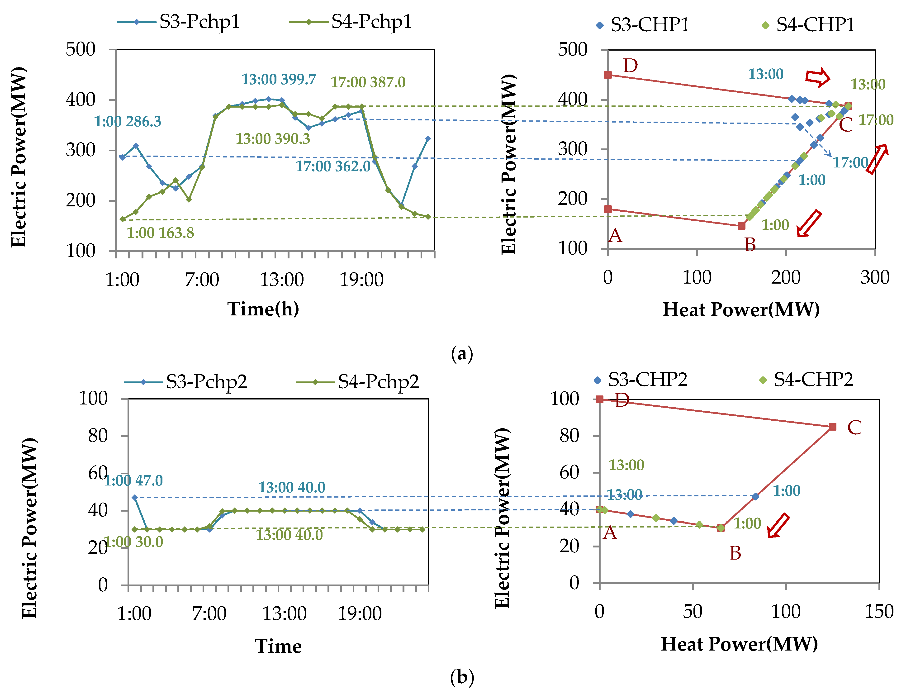
  • The annual operation and maintenance cost of the scenario with TTD-HN (S4), compared with the scenario without TTD-HN (S3), is reduced by CNY 21.49 million—a decrease of 3.54%;
  • The configuration heat capacity and HEX capacity of S4 compared with S3 is greatly reduced, and the annual investment cost is reduced by ¥8.709 million, or 59.4%. At the same time, the heat node selection of S4 is completely different from S3.
Firstly, the difference in the annual operation and maintenance costs is analyzed. Table 3 shows the cost components of scenarios S3 and S4. It can be seen that, after considering TTD-HN, all components are reduced, where the CHP1 cost and wind curtailment penalty cost are reduced the most, accounting for 39.4% and 35.0% of the annual operation and maintenance cost reductions, respectively. The reasons for these two cost reductions are analyzed below.
After considering TTD-HN in S4, the coordination regulation ability between the heat network and WTES is greatly enhanced, achieving a larger-scale heat transfer at different times of the day. Figure 6 shows the optimal results of heat power scheduling. The typical day can be divided into the night period of 20:00–8:00 and the day period of 9:00–19:00. Due to the lack of a TTD-HN model, the heat network in S3 does not have a regulation ability, and so the heat transfer quantity between night and day periods is 540 MWh, and is only relying on WTES. In S4, the heat transfer quantity of the heat network is 712.5 MWh, and the heat transfer quantity of WTES is 178.8 MWh. It can be seen that, with the TTD-HN model, on the one hand, the regulation ability of the heat network is greatly enhanced and, on the other hand, the demand for WTES is reduced.
The enhancement of the regulation ability provides a more flexible optimization space for the CHP units, and the CHP operational economy is improved. Figure 7 shows the operation status of the CHP units.
With a comparison of the operation status of the CHP units, we can see the following:
  • During the night period, the state points of the two CHP units in S4 are closer to point B (CHP1: (150, 145.8); CHP2: (65, 30)) than those in S3, which provides more space for wind power utilization and reduces fuel consumption. Taking 1:00 as an example, the electric power of CHP1 in S4 is 163.8 MW, and the fuel consumption is 89.7 tons of standard coal per hour, which is 122.5 MW and 26.5 tons/h lower than S3. The electric power of CHP2 is 30.0 MW, and the fuel consumption is 18,900 m3 of natural gas per hour, which is 17.0 MW and 23,100 m3/h lower than S3. According to the statistics, the annual operating and maintenance cost of CHP1 and CHP2 units at night are reduced by ¥12.619 million and ¥1.816 million.
  • During the day period, although the operation cost of CHP1 increases in S4, the efficiency improves. The average efficiency of CHP1 is increased from 4.610 MWh/tons (heat generation: 1.760 MWh/tons + electric generation: 2.850 MWh/tons) in S3 to 4.722 MWh/tons (heat generation: 1.905 MWh/tons + electric generation: 2.817 MWh/tons). In this period, the electricity generation of CHP1 increases by 53.9 MWh and the heat generation increases by 322.1 MWh, while the annual operating cost increases by ¥4.158 million, or 33% of the cost reduction during the night. CHP2 mainly undertakes peak heat load regulation at night, and its daytime operation state points are basically unchanged.
Figure 8 shows the changes of wind power and utilization rate under the two scenarios. It can be seen that the wind power of S4 increases by 155.3 MW, 139.9 MW, 131.6 MW, and 60.5 MW from 24:00 to 3:00 when the wind curtailment is the most serious. Additionally, the wind power utilization rate increases by 92.4%, 69.9%, 65.8%, and 38.8%. According to the statistics, the wind power generation of S4 on a typical day increases by 627.5 MWh, the wind power utilization rate increases by 28.7%, and the annual wind curtailment penalty cost decreases by ¥7.53 million.
Next, the node selection and heat capacity of WTES is analyzed. It is found that WTES is always configured in the node with the best effect of enhancing the adjustment ability of the heat system in both scenarios. The difference is that S3 is configured in the node with the largest heat load, while S4 is configured in the node with an excessively low or high operation temperature.
In S3, the node with the largest heat load has the largest mass flow. Under the same temperature change, a node with a large load and large mass flow can provide more heat exchange power. Compared with other nodes, DTES as configured here can give full play to the ability of heat transfer and improve the cost of the system; therefore, four heat nodes—H21, H22, H23 and H28—with the largest heat load are selected.
In S4, the heat network takes on the main role of heat transfer. At this time, the nodes with an excessively low or high operating temperature have a more restrictive effect on the heat network regulation ability. Figure 9 shows the return temperature curves of H18, H24, and H28 under S2 and S4, and the heat power change of WTES at H18 under S4. The heat discharging power is positive and the charging power is negative.
It can be seen from Figure 9 that in S2 without DTES, the night period return temperature of H18 is lower than that of H24 and H28. Especially, at 24:00–7:00, the temperature is close to the minimum value of 60 °C. Thus, at 23:00–6:00, the supply temperature of HSS cannot be further adjusted downward, and the heat power output of the units is limited. Similarly, in S2, the day return water temperature of H18 is close to the maximum value of 80 °C. Thus, at 13:00–9:00, the output of the HSS cannot be further adjusted upward, and the regulation ability of the heat power output is limited. The return temperature constraints can be effectively broken by installing WTES. The heat discharging power in the night period can increase the return temperature, and the heat charging power in the day period can decrease the return temperature, which enhances the heat regulation ability of the CHP and provides the CHP with more flexible operation space.
Figure 10 shows the change of configuration schemes in the solution space during the optimization process of the immune algorithm. The red dot indicates the final optimization result. It can be seen that with the increase of WTES investment cost, the annual operation and maintenance cost gradually decreases, and the annual total cost first decreases and then increases. The minimum value of the total cost corresponds to the final configuration scheme. At the same time, because the heat network in S4 undertakes most of the heat power transfer, the heat capacity of WTES is reduced, resulting in an annual investment of ¥5.958 million, which is far lower than the ¥14.667 million in S3.

5.1.2. Influence of Medium Temperature Characteristics of Distributed Thermal Energy Storage on the Configuration Scheme

This section constructs a new scenario, NS4, for comparative analysis. The configuration scheme of DTES in NS4 is the same as that in S4, but the MTC-DTES model is introduced into the lower stage optimization for the typical day. Through the comparison of results of S4, NS4, and S5, the influence of the MTC-DTES on the configuration is illustrated.
Table 4 shows the costs of S4, NS4 and S5 configuration schemes. Comparing the costs in Table 4, it can be found that the annual operation and maintenance cost of S5 is ¥1.687 million greater than that of S4, and the comprehensive annual total cost is ¥1.153 million greater. Compared with NS4, the annual operating and maintenance cost and comprehensive annual total cost of S5 are smaller, and the two costs are reduced by ¥0.563 million and ¥1.097 million. At the same time, the annual investment cost is reduced by ¥0.534 million, or 8.96%.
Without the MTC-DTES model, in S4, the medium temperature of the primary heat network flowing into the WTES HEX is considered to be constant, which is the designed supply temperature of 120 °C. However, in the actual operation, the medium temperature changes between 95–120 °C, resulting in the actual economic performance of NS4 not reaching a value in S4 which is as good as expected.
In Figure 11a, the curve Hwtes shows the hourly heat power output, ChMax shows the maximum heat charging power, and DisMax shows the maximum heat discharging power curve of WTES at H4 under three scenarios. Figure 11b shows the heat proportion of WTES, which is the proportion of actual heat quantity to configuration heat capacity.
It can be seen from Figure 11 that the actual heat charging power in NS4 is lower than S4 at most time intervals, and the maximum decrease is 3.76 MW at 14:00, with a decrease rate of 43%. The decrease heat charging power leads to a decrease in the actual heat quantity in the water tank. The maximum actual heat quantity accounts for 88.5% of the configured heat capacity, which is reduced by 6.5% compared with S4. According to the statistics, 4.7 MWh of configured capacity is not utilized. The configuration scheme of S5 avoids these problems. First of all, the HEX capacity K F 1 W T E S is generally larger than that of NS4, which enhances the heat exchange ability with the primary heat network, and the heat charging power at 14:00 is 1.14 MW higher than that of NS4. Secondly, the configuration heat capacity is reduced by 10 MWh, and there is no more wastage of capacity. Finally, the configuration HEX capacity s K F 2 W T E S is reduced. On the one hand, this weakens the ability to discharge heat to users, resulting in an increase of ¥0.139 million in the annual operation and maintenance cost of the CHP in the night period and ¥0.128 million from the wind curtailment penalty cost; on the other hand, this reduces the annual investment cost by ¥0.458 million. From these two aspects, the reduction of the HEX capacity improves the economic performance.

5.2. Distributed Thermal Energy Storage Types

In order to analyze the influence of WTES and EH-PHTES on the configuration scheme, the following two scenarios are added on the premise of considering the medium temperature characteristics:
  • S6: Only EH-PHTES is equipped;
  • S7: WTES and EH-PHTES are configured together.
The electric power used for electric heating comes from the power nodes near the HES system. The corresponding relationship between power and heat nodes is shown in Appendix A, Table A5. A mixture of palmitic acid and stearic acid is selected as a specific phase change material, and a small amount of carbon materials is added to enhance the heat transfer ability [56,57]. The phase change temperature is 65 °C. The cost per megawatt-hour is about one million. Table 5 shows the configuration results of scenarios S5–S7.
From the analysis of different configuration schemes of DTES types, the following can be seen:
  • In the three scenarios, H4, H18, and H19 are selected to configure DTES because of their large restriction of the regulation ability of the heat network. In scenarios S6 and S7, the H22–E25 node is selected to configure EH-PHTES, because H22–E25 is the closest electricity and heat load coupling node to the wind farm. Configuring EH-PHTES here can make use of the wind power nearby;
  • Compared with S5, the annual operating and maintenance cost of S6 decreases by ¥1.499 million, the annual investment cost increases by ¥2.011 million, and the annual total cost is ¥0.512 million greater. Compared with S5, the annual operating and maintenance cost of S7 is reduced by ¥1.041 million, the annual investment cost is increased by ¥0.534 million, and the annual total cost is reduced by ¥0.506 million.
Table 6 shows the components of the operating and maintenance costs in three scenarios.
The following can be seen from Table 6:
  • In S5, the costs of CHP1 and CHP2 units, TPG units and DTES are the lowest among the three scenarios, and the total cost is reduced by ¥0.801 million and ¥0.217 million, respectively, compared with S6 and S7. This is because WTES can not only discharge in the night period but also charge in the day period, which has the strongest effect on improving the regulation ability of the heat network. Additionally, EH-PHTES can only discharge to the heat network, so the regulation ability of the heat network is limited;
  • The wind curtailment penalty cost in S6 is the lowest in three scenarios, at ¥2.298 million and ¥1.041 million lower than that in S5 and S7. This is because EH-PHTES can directly use wind power for heating, which is more conducive to wind power consumption;
  • In the S7 configuration scheme, three nodes (H4, H18, H19) with a severe restriction on the improvement of the heat network regulation ability are selected to configure WTES, and the node (H22–E25) with the most direct use of wind power is selected to configure EH-PHTES. The advantages of the two types of DTES are fully reflected to optimize the operation cost, and the investment cost is not excessively high. Thus, the comprehensive annual total cost is the lowest of the three scenarios.

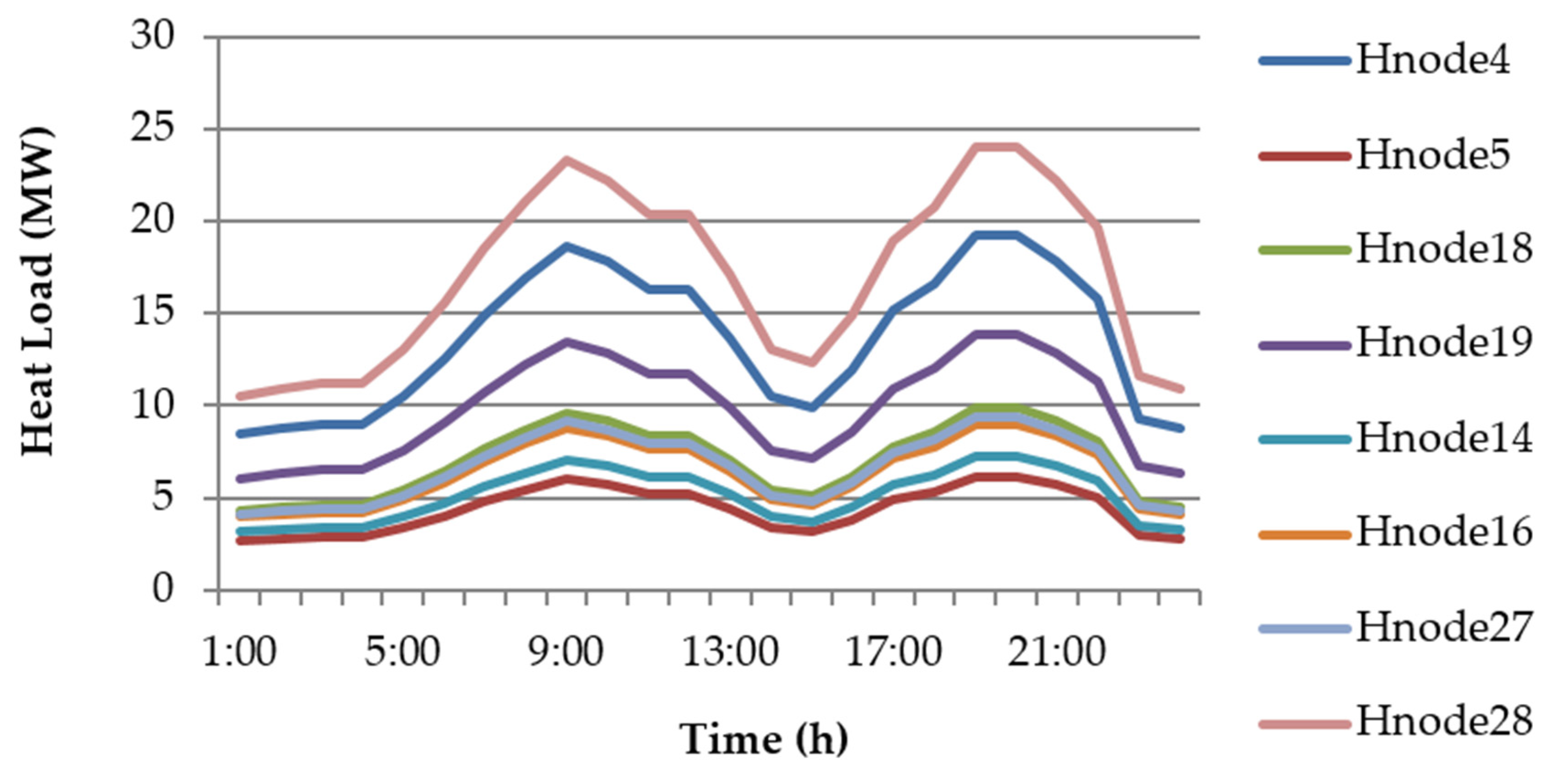
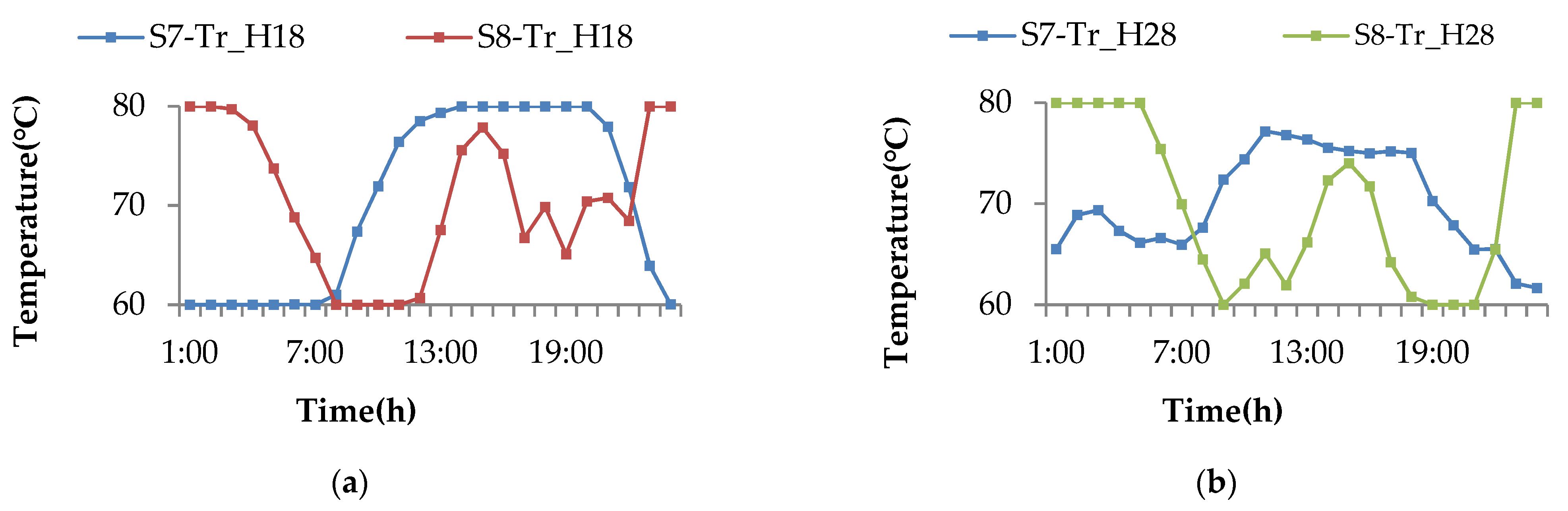
5.3. Heat Load Types

In this section, a kind of commercial building heat load, which is different from the UEHIES heat load curve, is set up in different nodes to explore the influence of different heat load types on the configuration scheme. The heat load curve of commercial buildings is shown in Appendix A, Figure A1. Therefore, two new scenarios are added:
  • S8: The commercial heat load is set at the head nodes H4, H5, H18, and H19;
  • S9: The commercial heat load is set at the end nodes H14, H16, H27, and H28.
Table 7 shows the configuration schemes of S7–S9.
It can be seen in Table 7 that, compared with S7, the three nodes, H4, H18, and H19, are no longer equipped with DTES in S8 and S9, while the three nodes, H20, H21, and H22, and four nodes, H14, H16, H27, and H28, are selected. In addition, the heat capacity and HEX capacity also change in each scenario. This is mainly because the operating temperature of HES, especially the return temperature, changes with the change of heat load types. Thus, the nodes that restrict the regulation ability of the heat network have changed. In order to improve the regulation ability in the new scenario, it is necessary to install DTES in the new severe restriction nodes, and the heat and HEX capacity will be adjusted accordingly.
For illustration, Figure 12a shows the return temperature of the H18 node under S7 and S8, and Figure 12b shows the return temperature of the H28 node under S7 and S9.
It can be seen from Figure 12a that under S7, the return temperature of H18 is too low in the night period and too high in the day period. However, in S8, the return temperature of H18 increases at night and decreases during the daytime; thus, it is no longer a severe restriction node, so there is no need to configure DTES. At the same time, it can be seen from Figure 12b that in S7, the return temperature of H28 is neither too high nor low. However, in S8, the return temperature of H28 increases in the night period, especially at 23:00–2:00, when it reaches the upper constraints, which limits the increase of the heat power of the CHP in the corresponding period of 15:00–20:00; at the same time, the return temperature drops in the day period, reaching the lower constraints at 9:00, which limits the decrease in the heat power of the CHP in the corresponding period of 2:00–3:00. H28 thus becomes a severe restriction node, which seriously limits the regulation capacity of the heat network. Therefore, H28 needs to be equipped with DTES under new heat load types. The situation for other configuration nodes is similar.

5.4. Wind Power Capacity

According to the analysis in Section 5.2, the advantage of EH-PHTES is wind power utilization. In order to analyze the impact of wind power capacity on the configuration scheme, two new scenarios are set in this section as follows:
  • S10: The capacity of wind power is set to 100 MW;
  • S11: The capacity of wind power is set to 300 MW.
Table 8 shows the configuration schemes of S7, S10, and S11. In order to reflect the wind power utilization, new columns are added in the table, and the calculation of new columns is given in Appendix B.
According to the analysis of the configuration schemes under different wind power capacity, the following can be seen:
  • With the wind power capacity of S10, S7, and S11 increasing in turn, the wind power utilization gradually increases and the annual operation and maintenance cost of the units gradually decreases; however, at the same time, the wind curtailment penalty cost increases. This is because in the day period, wind farms and CHP and TPG units share the power load supply and give priority to clean and cheap wind power output. With the increase of wind power capacity, the wind power generation and utilization quantity increase, the power outputs of CHP and TPG units decrease, fuel consumption decreases, and the annual operation and maintenance cost decreases. However, at night, there is insufficient utilization space for wind power. With the increase in capacity, the wind curtailment power increases and the annual cost of the wind curtailment penalty increases.
  • With the increase of wind power capacity, the amount of EH-PHTES, the heat and HEX capacity, and the rated power of EH increase. This is because the increase of wind curtailment power is more conducive to the EH-PHTES system realizing its potential to use nearby wind power. In order to make more use of wind power, the number of EH-PHTES systems and the capacity of each component are required to increase continuously to improve the wind power utilization. However, this also causes an increase in the investment cost.

5.5. Centralized Thermal Energy Storage

Centralized thermal energy storage is configured at the HSS node to regulate the heat medium flowing into the primary heat network [58]. In order to explore the difference between centralized and distributed thermal energy storage, a new scenario is set in this section: S12—configure WTES equipment in the HSS.
Table 9 shows the configuration results of S5 (a distributed WTES configuration) and S12.
The analysis of the centralized and distributed configuration scheme shows that the heat capacity of the centralized scheme is 130 MWh higher than the total heat capacity of the distributed scheme, and the HEX capacity is 1.8 MW/°C higher. A centralized storage device can decouple the heat demand and the HSS heat output to some extent, meaning that the operation schedule of the CHP units can be optimized. However, compared with DTES, it is not effective at improving the regulating ability of the heat network. Therefore, if roughly the same operation and maintenance cost is incurred, the annual investment cost of the centralized scheme is ¥4.736 million greater. It is shown that, compared with the centralized configuration, DTES is more conducive to saving investment costs.

6. Conclusions

In this paper, a model of DTES considering the medium–temperature characteristics is established; afterwards, an optimal economic configuration method in a UEHIES is proposed that takes the TTD-HN and MTC-DTES models into account. Through the analysis of different scenarios, the following conclusions are drawn.
(1)
Considering TTD-HN, the heat network can be effectively utilized, the heat capacity and HEX capacity can be reduced, and the investment cost can be reduced. At the same time, considering MTC-DTES can avoid the waste of configuration heat capacity and reduce the actual operation and maintenance costs;
(2)
Compared with the centralized configuration, the heat and HEX capacity of DTES is significantly decreased, the thermal energy storage investment cost is reduced, and the economic factors of the system are improved;
(3)
WTES has a stronger effect on improving the regulation ability of the heat network and EH-PHTES is more conducive to improving the wind power utilization. The capacity of wind power is a major factor when determining the configuration scheme of EH-PHTES;
(4)
Different types and distributions of heat load directly affect the temperature of HES, resulting in the change of the location and number of nodes that severely restrict the regulating ability of the heat network, thus changing the configuration nodes and investment cost of DTES.
Future work will include the characteristic extraction method of TMR data to reduce the error rate.

Author Contributions

Conceptualization, supervision, writing—review and editing, and funding acquisition, W.W.; methodology, software, and writing—original draft, Y.G.; writing—review and editing, K.H., Y.S. and K.Y.; funding acquisition, H.J. and C.S.; resources, K.H. All authors have read and agreed to the published version of the manuscript.

Funding

This work was supported by the Science and Technology Project of State Grid Corporation of China (SGSDJY00GPJS1900058).

Institutional Review Board Statement

Not applicable.

Informed Consent Statement

Not applicable.

Data Availability Statement

The data presented in this study are available on request from the corresponding author.

Conflicts of Interest

The authors declare no conflict of interest.

Nomenclature

Superscripts:
C H P Combined heat and power plant E H - P H T E S Electric heater phase change thermal energy storage
W T E S Water thermal energy storage N E T Heat network
T P G Thermal power generation H E S Heat exchange station
H S S Heat source station H E X Heat exchanger
O & M Operation and maintenance E H Electric heater
W Wind power W T E S Water thermal energy storage
D T E S Distributed thermal energy storage D I S Discharge heat power
C H Charge heat power
Subscripts:
i / j Node number s / r Supply/return pipe
t Time interval number m a x / m i n Maximum/minimum value
l Path number between HSS and HES u p p e r Upper value
k Corner point number of CHP l o w e r Lower value
1/2Primary/secondary heat network i n v Investment
Variables:
m N E T Mass flow of the heat network into HEX, kg/s m W T E S Mass flow of WTES pipe, kg/s
m i , t , 1 N E T Mass flow of the primary heat network into HEX in node i at time t, kg/s m i , 1 H E S Mass flow of HES connected to the primary heat network in node i, kg/s
m i , t , 2 N E T Mass flow of the secondary heat network into HEX in node i at time t, kg/s m i , 2 H E S Mass flow of HES connected to the secondary heat network in node i, kg/s
m P H T E S Mass flow of EH-PHTES circulating pipes, kg/s m i , 1 H S S Mass flow of HSS connected to the primary heat network in node i, kg/s
H N E T Heat power of the heat network, MW H H E X Heat power of HEX, MW
H W T E S Heat power of WTES, MW H E H - P H T E S Heat power of EH-PHTES, MW
H i , t W T E S , C H Heat charging power of WTES in node i at time t, MW H i , t E H - P H T E S , C H Heat charging power of EH-PHTES in node i at time t, MW
H i , t W T E S , D I S Heat discharging power of WTES in node i at time t, MW H i , t E H - P H T E S , D I S Heat discharging power of EH-PHTES in node i at time t, MW
T s N E T Temperature of the heat network transfer medium in HEX inlet, °C T r N E T Temperature of the heat network transfer medium in HEX outlet, °C
T u p p e r W T E S Temperature of WTES upper zone, °C T l o w e r W T E S Temperature of WTES lower zone, °C
T s , 1 H E S Temperature of HES supply pipe connected to the primary heat network, °C T ave , i W T E S Temperature of WTES water tank average value in node i, °C
T s , i , t , 1 H E S Temperature of HES supply pipe connected to the primary heat network in node i at time t, °C T r , i , t , 2 H E S Temperature of HES return pipe connected to the secondary heat network in node i at time t, °C
T E H - P H T E S Phase transition temperature of EH-PHTES, °C T d H E S Designed temperature of HES, °C
T s , i H S S Temperature of HSS supply pipe in node i, °C T r , i H S S Temperature of HSS return pipe in node i, °C
T a Temperature of ambient, °C T n Indoor temperature, °C
Δ T x Temperature difference at HEX outlet, °C Δ T d Temperature difference at HEX inlet, °C
K F 1 W T E S Capacity of WTES HEX connected to the primary heat network, MW/°C K F The actual heat transfer capacity of HEX, MW/°C
K F 2 E H - P H T E S Capacity of EH-PHTES HEX connected to the secondary heat network, MW/°C K F m a x W T E S Maximum of WTES HEX configuration capacity, MW/°C
K F 2 W T E S Capacity of WTES HEX connected to the secondary heat network, MW/°C K F m a x E H - P H T E S Maximum of EH-PHTES HEX configuration capacity, MW/°C
R i , t , 1 W T E S Thermal resistance of WTES connected to the primary heat network in node i at time t, °C/MW N o n E H P H T E S The number n EH-PHTES configuration node
R i , t , 2 E H P H T E S Thermal resistance of EH-PHTES connected to the secondary heat network in node i at time t, °C/MW N o n W T E S The number n WTES configuration node
R i , t , 2 W T E S Thermal resistance of WTES connected to the secondary heat network in node i at time t, °C/MW Γ W T E S Set of WTES configuration nodes
Γ E H - P H T E S Set of EH-PHTES configuration nodes. Γ A N W T E S Set of WTES alternative configuration nodes
Γ A N E H - P H T E S Set of EH-PHTES alternative configuration nodes. Γ C H P Set of CHP units
Γ T P G Set of TPG units Γ W Set of wind farms
Γ D T E S Set of DTES Γ D a y Set of typical day numbers
Γ l , p i p e Set of pipes that the path l passes through Γ t Set of time interval number
Γ l , n o d e Set of pipes/nodes that the path l passes through Γ i j Set of paths from node i to node j
S c a p , m a x P H T E S Maximum of EH-PHTES configuration capacity, MWh S c a p , m a x W T E S Maximum of WTES configuration capacity, MWh
S i , m i n W T E S Minimum of WTES heat quantity in node i, MWh S i , m a x W T E S Maximum of WTES heat quantity in node i, MWh
S i , m i n P H T E S Minimum of EH-PHTES heat quantity in node i, MWh S i , m a x P H T E S Maximum of EH-PHTES heat quantity in node i, MWh
S c a p , i W T E S Heat capacity of WTES tank in node i, MWh S i , t W T E S Quantity of heat in WTES in node i at time t, MWh
S c a p , i P H T E S Heat capacity of EH-PHTES storage tank in node i, MWh S i , t P H T E S Quantity of heat in EH-PHTES in node i at time t, MWh
H C H P Heat power of CHP, MW P C H P Electric power of CHP, MW
H k C H P Heat power of CHP at corner point k, MW P k C H P Electric power of CHP at corner point k, MW
Γ k Set of corner point k Γ i C H P Set of CHP in node i
H L i , t H E S Heat load of HES in node i at time t, MW P i , t Electric active power in node i at time t, MW
Q i , t Electric reactive power in node i at time t, MW P L o a d Electric active load, MW
P R a t e d E H Rated power of EH, MW Δ P R a m p Maximum ramping power, MW/h
P R a t e d , m a x E H Maximum rated power of EH, MW P i , t E H Electric power of EH in node i at time t, MW
P i , t W , p r e Predicted wind power in node i at time t, MW P i , t W , r e a l Real wind power in node i at time t, MW
P i , t W , c u r Wind curtailment power in node i at time t, MW P r W Wind power capacity, MW
Q L o a d Electric reactive load, MVar C i n v a n n Annual investment cost, ¥
C T o t a l a n n Comprehensive annual total cost, ¥ C i n v , i W T E S Investment cost of WTES in node i, ¥
C O & M a n n Annual operation and maintenance cost, ¥ C t C H P Operation cost of CHP at time t, ¥
C i n v , i E H - P H T E S Investment cost of EH-PHTES in node i, ¥ C t W Wind curtailment cost at time t, ¥
C t T P G Operation cost of TPG at time t, ¥ U Node voltage, p.u.
C t D T E S Operation and maintenance cost of DTES at time t, ¥ v i , t Speed of wind farm in node i at time t, m/s
Parameters:
G Real part of node admittance matrix B Imaginary part of node admittance matrix
G Real part of node admittance matrix without grounding branches B Imaginary part of node admittance matrix without grounding branches
α Combination coefficients of CHP ξ Temperature transfer coefficient
Φ p Temperature loss coefficient of pipe p δ q Temperature distribution coefficient of node q
γ l Time delay of path l , h b Radiator coefficient of thermal users
f G The fuel consumption of TPG, t/MWh Δ t Dispatch time interval, h
r Discount rate, % y Design service life, year
D Number of general days represented by typical day in a year, day η E H Electric to thermal efficiency of EH, %
t 0 The initial time interval t e n d The final time interval
c f Specific heat capacity of heat medium, kJ/(kg·°C) c f u e l Price of fuel, ¥/t
ρ Medium density, kg/m3 c c a p Price of heat quantity capacity, ¥/MWh
c W Price of wind curtailment, ¥/MWh c k C H P Price of CHP unit at corner point k, ¥/h
c H Maintenance price of equipment heat power, ¥/MWh c P E H Price of EH capacity, ¥/MW
c P Maintenance price of equipment electric power, ¥/MWh c K F Price of heat exchanger, ¥/(MW/°C)
L f P H T E S Latent heat of phase change material, kWh/kg V E H - P H T E S Volume of phase change material, m3
f P H T E S Liquid ratio of PHTES, % V W T E S Volume of WTES water tank, m3
v c u t - i n Cut-in speed of wind generator, m/s v c u t - o u t Cut-out speed of wind generator, m/s
v r a t e d Rated speed of wind generator, m/s γ l Rounded-up value of γ l
γ l Rounded-down value of γ l

Appendix A

Table A1. Heat network node parameters.
NodeTypeHL(MW)Delay(h)m(kg/s)NodeTypeHL(MW)Delay(h)m(kg/s)
130.00 1510.00
210.00 1618.056.45947.92
310.00 1710.00
4117.201.060102.381818.841.03252.62
515.511.74232.8019112.391.42573.75
6114.612.68386.9620119.921.641118.57
7120.222.820120.3621127.571.978164.11
8112.422.96073.9322134.162.374203.33
9110.553.53262.8023128.443.049169.29
1010.00 24111.233.87366.85
1119.684.22257.6325116.934.612100.77
1217.634.37345.4226110.405.54461.90
1318.974.67253.392718.415.98650.06
1416.484.90838.5728121.446.540127.62
Table A2. Heat network pipe parameters.
NoF_NoT_NoLength
(m)
Diameter
(m)
m
(kg/s)
Conductivity
(W/(m·°C)
Roughness
(m)
112100011911.0180.20.005
2232264.51722.1490.20.005
3348651722.1490.20.005
44519391619.7680.20.005
55625311586.9700.20.005
6673151500.0060.20.005
7783000.9379.6490.20.005
8899900.9305.7200.20.005
99106890.9242.9230.20.005
1010112590.9242.9230.20.005
1111122000.8185.2980.20.005
1212133000.8139.8810.20.005
1313142600.686.4880.20.005
1414154020.647.9170.20.005
15151616000.3547.9170.20.005
16217250011188.8690.20.005
171718250011188.8690.20.005
181819205011136.2500.20.005
191920105011062.5000.20.005
20202118000.9943.9290.20.005
21212217500.9779.8210.20.005
22222322000.9576.4880.20.005
23232419000.9407.2020.20.005
24242518000.8340.3570.20.005
25252616000.8239.5830.20.005
26262710000.6177.6790.20.005
2727289000.6127.6190.20.005
Table A3. CHP operation parameter.
Corner Points H C H P (MW) P C H P (MW) F u e l C H P (tons/h) c C H P (CNY/h)
CHP1A018055.827,900
B150145.885.7842,891
C270387137.9868,985
D045013567,500
Corner Points H C H P (MW) P C H P (MW) F u e l C H P (m3/h) c C H P (CNY/h)
CHP1A04013,33334,667
B653018,88949,111
C1258542,000109,200
D010025,00065,000
Table A4. Parameter values in the optimization process.
Q M A X W T E S 95 % Q c a p W T E S Q M A X P H T E S 95 % Q c a p P H T E S b 0.35
Q M I N W T E S 5 % Q c a p W T E S Q M I N P H T E S 5 % Q c a p P H T E S r 0.08
T u p p e r W T E S 95 °C T P H T E S 65 °C y 20 years
T l o w e r W T E S 60 °C c c a p P H T E S ¥1,000,000 c f 4.2 k J / ( k g ° C )
c c a p W T E S ¥150,000 c K F P H T E S ¥15,000,000 T n 20 °C
c K F W T E S ¥15,000,000 c P E H ¥1,500,000 η E H 100%
c H , M ¥20 c P / H , M ¥20 T s , d , 2 H E X / T r , d , 2 H E X 75 °C/40 °C
S c a p , m a x W T E S 160 MWh S c a p , m a x P H T E S 50 MWh T r , u p p e r / T r , l o w e r 80 °C/60 °C
K F m a x , 1 W T E S 2.0 MW/°C K F m a x P H T E S 2.0 MW/°C T s , u p p e r / T s , l o w e r 120 °C/95 °C
K F m a x , 2 W T E S 2.0 MW/°C P R a t e d , m a x E H 50 MW
Table A5. Coupling of electric and heat nodes.
Heat Node4567891112131416
Electric Node11222130301919292827
Heat Node1819202122232425262728
Electric Node3872525242413141517
Figure A1. Commercial building heat load.
Energies 14 02924 g0a1

Appendix B

The wind power consumption of a typical day W C o n is the total quantity of wind power utilization at every wind farm at every time interval.
W C o n = i Γ W t Γ t P i , t W , r e a l Δ t
The wind power consumption W D T E S C o n is derived from W C o n on a typical day with DTES configured. Wind power consumption W N o _ D T E S C o n is derived from W C o n on a typical day without DTES. The increase of wind power consumption on a typical day W I n c C o n is the difference of W D T E S C o n and W N o _ D T E S C o n .
W I n c C o n = W D T E S C o n W N 0 _ D T E S C o n
The annual wind curtailment penalty cost is shown as follows:
W W C A n n = d Γ D a y ( D d t Γ t , d C t , d W )
The annual operation and maintenance cost of other units is shown as follows:
W u n i t A n n = d Γ D a y [ D d t Γ t , d ( C t , d C H P + C t , d T P G + C t , d D T E S ) ]

References

  1. Abbott, D. Keeping the energy debate clean: How do we supply the world’s energy needs? Proc. IEEE 2010, 98, 42–66. [Google Scholar] [CrossRef]
  2. Kober, T.; Schiffer, H.-W.; Densing, M.; Panos, E. Global energy perspectives to 2060—WEC’s World Energy Scenarios 2019. Energy Strat. Rev. 2020, 31, 100523. [Google Scholar] [CrossRef]
  3. GWEC. Global Wind Report 2019. Available online: https://gwec.net/docs/global-wind-report-2019/ (accessed on 1 September 2020).
  4. Wu, J.; Yan, J.; Jia, H.; Hatziargyriou, N.; Djilali, N.; Sun, H. Integrated Energy Systems. Appl. Energy 2016, 167, 155–157. [Google Scholar] [CrossRef]
  5. Mancarella, P. MES (multi-energy systems): An overview of concepts and evaluation models. Energy 2014, 65, 1–17. [Google Scholar] [CrossRef]
  6. Li, G. Sensible heat thermal storage energy and exergy performance evaluations. Renew. Sustain. Energy Rev. 2016, 53, 897–923. [Google Scholar] [CrossRef]
  7. Kousksou, T.; Jamil, A.; El Rhafiki, T.; Zeraouli, Y. Paraffin wax mixtures as phase change materials. Sol. Energy Mater. Sol. Cells 2010, 94, 2158–2165. [Google Scholar] [CrossRef]
  8. Alva, G.; Lin, Y.; Fang, G. An overview of thermal energy storage systems. Energy 2018, 144, 341–378. [Google Scholar] [CrossRef]
  9. Vandermeulen, A.; Van Der Heijde, B.; Helsen, L. Controlling district heating and cooling networks to unlock flexibility: A review. Energy 2018, 151, 103–115. [Google Scholar] [CrossRef]
  10. Schuchardt, G.K. Integration of decentralized thermal storages within District Heating (DH) Networks. Environ. Clim. Technol. 2016, 18, 5–16. [Google Scholar] [CrossRef] [Green Version]
  11. Jebamalai, J.M.; Marlein, K.; Laverge, J. Influence of centralized and distributed thermal energy storage on district heating network design. Energy 2020, 202, 117689. [Google Scholar] [CrossRef]
  12. Victoria, M.; Zhu, K.; Brown, T.; Andresen, G.B.; Greiner, M. The role of storage technologies throughout the decarbonisation of the sector-coupled European energy system. Energy Convers. Manag. 2019, 201, 111977. [Google Scholar] [CrossRef] [Green Version]
  13. Good, N.; Mancarella, P. Flexibility in multi-energy communities with electrical and thermal storage: A stochastic, robust approach for multi-service demand response. IEEE Trans. Smart Grid 2017, 10, 503–513. [Google Scholar] [CrossRef]
  14. Patteeuw, D.; Bruninx, K.; Arteconi, A.; Delarue, E.; D’haeseleer, W.; Helsen, L. Integrated modeling of active demand re-sponse with electric heating systems coupled to thermal energy storage systems. Appl. Energy 2015, 151, 306–319. [Google Scholar] [CrossRef] [Green Version]
  15. Good, N.; Karangelos, E.; Navarro-Espinosa, A.; Mancarella, P. Optimization under uncertainty of thermal storage-based flexible demand response with quantification of residential users’ discomfort. IEEE Trans. Smart Grid 2015, 6, 2333–2342. [Google Scholar] [CrossRef]
  16. Marguerite, C.; Andresen, G.B.; Dahl, M. Multi-criteria analysis of storages integration and operation solutions into the dis-trict heating network of Aarhus—A simulation case study. Energy 2018, 158, 81–88. [Google Scholar] [CrossRef]
  17. Dincer, I.; Ezan, M.A. Thermal energy storage applications. In Heat Storage: A Unique Solution for Energy Systems; Springer: Cham, Switzerland, 2018; pp. 85–135. [Google Scholar]
  18. Zhang, L.; Xiong, X.; Hu, J. Operation of a Microgrid System with Distributed Energy Resources and Storage. Lect. Notes Elect. Eng. 2015, 313, 495–502. [Google Scholar]
  19. Kong, X.; Bai, L.; Hu, Q.; Li, F.; Wang, C. Day-ahead optimal scheduling method for grid-connected microgrid based on energy storage control strategy. J. Mod. Power Syst. Clean Energy 2016, 4, 648–658. [Google Scholar] [CrossRef] [Green Version]
  20. Guillén-Lambea, S.; Carvalho, M.; Delgado, M.; Lazaro, A. Sustainable enhancement of district heating and cooling configurations by combining thermal energy storage and life cycle assessment. Clean Technol. Environ. Policy 2021, 23, 857–867. [Google Scholar] [CrossRef]
  21. Thomson, A.; Claudio, G. The Technical and Economic Feasibility of Utilising Phase Change Materials for Thermal Storage in District Heating Networks. Energy Proc. 2019, 159, 442–447. [Google Scholar] [CrossRef]
  22. Xin-Rui, L.; Fu-Jia, Z.; Qiu-Ye, S.; Peng, J. Location and Capacity Selection Method for Electric Thermal Storage Heating Equip-ment Connected to Distribution Network Considering Load Characteristics and Power Quality Management. Appl. Sci. 2020, 10, 2666. [Google Scholar]
  23. Guo, Y.; Wang, C.; Shi, Y.; Guo, C.; Shang, J.; Yang, X. Comprehensive optimization configuration of electric and thermal cloud energy storage in regional integrated energy system. Power Syst. Technol. 2020, 44, 1611–1623. [Google Scholar]
  24. Li, Z.; Wu, W.; Shahidehpour, M.; Wang, J.; Zhang, B. Combined heat and power dispatch considering pipeline energy storage of district heating network. IEEE Trans. Sustain. Energy 2016, 7, 12–22. [Google Scholar] [CrossRef]
  25. Cheng, H.; Wu, J.; Luo, Z.; Zhou, F.; Liu, X.; Lu, T. Optimal Planning of Multi-Energy System Considering Thermal Storage Capacity of Heating Network and Heat Load. IEEE Access 2019, 7, 13364–13372. [Google Scholar] [CrossRef]
  26. Li, Z.; Wu, W.; Wang, J.; Zhang, B.; Zheng, T. Transmission-Constrained Unit Commitment Considering Combined Electricity and District Heating Networks. IEEE Trans. Sustain. Energy 2016, 7, 480–492. [Google Scholar] [CrossRef]
  27. Zhao, B.; Zhang, X.; Ni, C.; Mu, Y.; Wang, M.; Meng, X. Optimal Scheduling Method for Electrical-Thermal Integrated Energy System Considering Heat Storage Characteristics of Heating Network. In Proceedings of the 2019 IEEE Innovative Smart Grid Technologies—Asia (ISGT Asia), Chengdu, China, 24 October 2019; p. 19093752. [Google Scholar] [CrossRef]
  28. Guo, Z.-Y.; Zhu, H.-Y.; Liang, X.-G. Entransy—A physical quantity describing heat transfer ability. Int. J. Heat Mass Transf. 2007, 50, 2545–2556. [Google Scholar] [CrossRef]
  29. Chen, Q.; Liang, X.-G.; Guo, Z.-Y. Entransy theory for the optimization of heat transfer—A review and update. Int. J. Heat Mass Transf. 2013, 63, 65–81. [Google Scholar] [CrossRef]
  30. Shen, Y.; Zhang, H.; Xu, H.; Yu, P.; Bai, T. Maximum heat transfer capacity of high temperature heat pipe with triangular grooved wick. J. Cent. South Univ. 2015, 22, 386–391. [Google Scholar] [CrossRef]
  31. Miha, B.; Bojan, G.; Iztok, G.; Ivan, B. Dynamic behaviour of a plate heat exchanger: Influence of temperature disturbances and flow configurations. Int. J. Heat Mass Transf. 2020, 163, 120439. [Google Scholar]
  32. Al-Dawery, S.K.; Alrahawi, A.M.; Al-Zobai, K.M. Dynamic modeling and control of plate heat exchanger. Int. J. Heat Mass Transf. 2012, 55, 6873–6880. [Google Scholar] [CrossRef]
  33. Wang, Y.; You, S.; Zheng, W.; Zhang, H.; Zheng, X.; Miao, Q. State space model and robust control of plate heat exchanger for dynamic performance improvement. Appl. Therm. Eng. 2018, 128, 1588–1604. [Google Scholar] [CrossRef]
  34. Chenhui, L.; Wenchuan, W.; Bin, W.; Mohammad, S.; Boming, Z. Joint Commitment of Generation Units and Heat Exchange Stations for Combined Heat and Power Systems. IEEE Trans. Sustain. Energy 2019, 11, 1118–1127. [Google Scholar]
  35. Zhao, C.; Lu, W.; Tian, Y. Heat transfer enhancement for thermal energy storage using metal foams embedded within phase change materials (PCMs). Sol. Energy 2010, 84, 1402–1412. [Google Scholar] [CrossRef] [Green Version]
  36. Inaba, H.; Kim, M.; Horibe, A. Melting Heat Transfer Characteristics of Microencapsulated Phase Change Material Slurries with Plural Microcapsules Having Different Diameters. J. Heat Transf. 2004, 126, 558–565. [Google Scholar] [CrossRef]
  37. Wang, L.; Su, J.; Ren, L. Preparation of thermal energy storage microcapsule by phase change. Polym. Mater. Sci. Eng. 2005, 21, 276–279. [Google Scholar]
  38. Lu, Q.; Hu, B.; Wang, H.; Zhang, N.; Liu, L. Heat-supply of thermal power plant in wind-heat conflict. Electr. Power. Autom. Equip. 2017, 37, 236–244. [Google Scholar]
  39. Danish Energy Agency. Technology Data for Energy Plants. Available online: https://ens.dk/sites/ens.dk/files/Statistik/technology_data_catalogue_for_el_and_dh_-_0009.pdf (accessed on 12 November 2020).
  40. Zheng, J.; Zhou, Z.; Zhao, J.; Wang, J. Integrated heat and power dispatch truly utilizing thermal inertia of district heating network for wind power integration. Appl. Energy 2018, 211, 865–874. [Google Scholar] [CrossRef]
  41. Lahdelma, R.; Hakonen, H. An efficient linear programming algorithm for combined heat and power production. Eur. J. Oper. Res. 2003, 148, 141–151. [Google Scholar] [CrossRef]
  42. Davide, A.; Francesco, C.; Ludovico, T. Wind Turbine Power Curve Upgrades. Energies 2018, 11, 1300. [Google Scholar]
  43. Cheon, J.; Kim, J.; Lee, J.; Lee, K.; Choi, Y. Development of Hardware-in-the-Loop-Simulation Testbed for Pitch Control System Performance Test. Energies 2019, 12, 2031. [Google Scholar] [CrossRef] [Green Version]
  44. Hassan, A.; Han, P.; Steven, R.W.; Beni, S. Cost–Benefit Analysis of HELE and Subcritical Coal-Fired Electricity Generation Technologies in Southeast Asia. Sustainability 2021, 13, 1591. [Google Scholar]
  45. Catalina, H.M.; Maria, T.C.G.; Alois, S.; Alvaro, L. Comparison between Concentrated Solar Power and Gas-Based Gener-ation in Terms of Economic and Flexibility-Related Aspects in Chile. Energies 2021, 14, 1063. [Google Scholar]
  46. Oleksii, E.; Vitalii, Z. Usage of biomass CHP for balancing of power grid in Ukraine. E3S Web Conf. In Proceedings of the 8th International Conference on Thermal Equipment, Renewable Energy and Rural Development, Targoviste, Romania, 20 August 2019; p. 02005. [Google Scholar] [CrossRef]
  47. Wei, W.; Shi, Y.; Hou, K.; Guo, L.; Wang, L.; Jia, H.; Wu, J.; Tong, C. Coordinated Flexibility Scheduling for Urban Integrated Heat and Power Systems by Considering the Temperature Dynamics of Heating Network. Energies 2020, 13, 3273. [Google Scholar] [CrossRef]
  48. Wang, D.; Zhi, Y.-Q.; Jia, H.-J.; Hou, K.; Zhang, S.-X.; Du, W.; Wang, X.-D.; Fan, M.-H. Optimal scheduling strategy of district integrated heat and power system with wind power and multiple energy stations considering thermal inertia of buildings under different heating regulation modes. Appl. Energy 2019, 240, 341–358. [Google Scholar] [CrossRef]
  49. Rafalskaya, T.A. Investigating the possibility of using low-temperature heat supply with the central qualitative regulation. Therm. Eng. 2019, 66, 858–867. [Google Scholar] [CrossRef]
  50. Dongli, Y.; Jun, C.; Congwei, T.; Zhilong, W.; Chen, L.; Hongfu, W. Optimal Energy Flow of Combined Electrical and Heating Multi-energy System Considering the Linear Network Constraints. Proc. CSEE 2019, 39, 1933–1944. [Google Scholar]
  51. Seyed, M.F.; Sajjad, A.G.B.G.; Seyed, H.H.; Mehrdad, A. Introducing a Novel DC Power Flow Method with Reactive Power Considerations. IEEE Trans. Power Syst. 2014, 30, 3012–3023. [Google Scholar]
  52. Mohammad, A.M.; Mohammad, H.; Kazem, Z.; Mehdi, A.; Behnam, M.-I.; Mousa, M.; Amjad, A.-M. A novel hybrid two-stage framework for flexible bidding strategy of reconfigurable micro-grid in day-ahead and real-time markets. Int. J. Electr. Power Energy Syst. 2020, 123, 106293. [Google Scholar]
  53. Yuanxing, X.; Qingshan, X.; Jun, Z.; Xiaodong, Y. Two-stage robust optimisation of user-side cloud energy storage configuration considering load fluctuation and energy storage loss. IET Gener. Transm. Distrib. 2020, 14, 3278–3287. [Google Scholar]
  54. Wang, C.; Yu, B.; Xiao, J.; Guo, L. Multi-scenario, multi-objective optimization of grid-parallel Microgrid. In Proceedings of the 2011 4th International Conference on Electric Utility Deregulation and Restructuring and Power Technologies (DRPT), Weihai, China, 6–9 July 2011. [Google Scholar] [CrossRef]
  55. MOHURD. Code for Urban Heating Supply Planning, 2nd ed.; China Architecture & Building Press: Beijing, China, 2015; pp. 12–51.
  56. Zhang, N. Properties Control and Heat Transfer Enhancement of Fatty Acids Phase Change Materials. Ph.D. Thesis, Southwest Jiaotong University, Chengdu, China, 2016. [Google Scholar]
  57. Zhang, N.; Yanping, Y.; Yaguang, Y.; Cao, X.; Yang, X. Effect of carbon nanotubes on the thermal behaviour of palmitic–stearic acid eutectic mixtures as phase change materials for energy storage. Sol. Energy 2014, 110, 64–70. [Google Scholar] [CrossRef]
  58. Chen, X.; Kang, C.; O’Malley, M.; Xia, Q.; Bai, J.; Liu, C.; Sun, R.; Wang, W.; Li, H. Increasing the Flexibility of Combined Heat and Power for Wind Power Integration in China: Modeling and Implications. IEEE Trans. Power Syst. 2015, 30, 1848–1857. [Google Scholar] [CrossRef]
Figure 1. Medium temperature zones and device connections of a WTES system.
Energies 14 02924 g001
Figure 2. Internal structure and the device connections of EH-PHTES.
Energies 14 02924 g002
Figure 3. Structure diagram of a typical UEHIES.
Energies 14 02924 g003
Figure 4. (a) Load curve and (b) predicted wind power curve.
Energies 14 02924 g004
Figure 5. Structure diagram of the UEHIES in the case study.
Energies 14 02924 g005
Figure 6. Optimal results of heat power scheduling on a typical day: (a) S3 and (b) S4.
Energies 14 02924 g006
Figure 7. Operation state of CHP units: (a) CHP1 and (b) CHP2.
Energies 14 02924 g007
Figure 8. Typical day wind power scheduling results: (a) wind power and (b) utilization rate.
Energies 14 02924 g008
Figure 9. Return temperature and WTES power of some nodes in S2 and S4.
Energies 14 02924 g009
Figure 10. The relationship between cost and investment: (a) annual operation and maintenance cost and annual investment cost of DTES; (b) comprehensive annual total cost and annual investment cost of DTES.
Energies 14 02924 g010
Figure 11. Operation state of WTES at node H4: (a) heat power and (b) heat proportion.
Energies 14 02924 g011
Figure 12. Before DTES is configured, the return temperature before and after the heat load curve changes: (a) H18 node and (b) H28 node.
Energies 14 02924 g012
Table 1. Settings for scenarios S1–S5.
ScenariosTTD-HNWTES Configuration MTC-DTES
S1NoNo--
S2YesNo--
S3NoYesNo
S4YesYesNo
S5YesYesYes
Table 2. Optimization results of configuration schemes of S1–S5.
ScenariosNode S c a p W T E S K F 1 W T E S K F 2 W T E S Annual Cost 1
C O & M a n n C I n v a n n C T o t a l a n n
S1--------65,362.9--65,362.9
S2--------59,873.3--59,873.3
S3H211600.40.560,687.61466.762,154.2
H221600.50.6
H231600.40.5
H281200.30.4
S4H4650.30.358,538.6595.859,134.4
H18350.10.2
H19400.20.2
H20600.30.3
S5H4550.40.258,707.3542.459,249.7
H18250.20.1
H19400.30.2
H20450.30.2
1 The cost column uses Chinese Yuan (CNY: ¥) 10,000 as a unit. The same unit is used in the other tables in Section 5.
Table 3. Composition of annual operation and maintenance cost of scenarios S3–S4.
ScenariosCHP1CHP2TPGWind CurtailmentDTES
S325,769.315,823.516,664.02025.7405.0
S424,923.215,641.916,565.11272.7135.7
Reduction846.1181.698.9753.0269.3
Table 4. Costs of S4, NS4 and S5 configuration schemes.
Scenarios C O & M a n n C I n v a n n C T o t a l a n n
S458,538.6595.859,134.4
NS458,763.6595.859,359.4
S558,707.3542.459,249.7
Table 5. Optimization results of configuration schemes of S5–S7.
ScenariosNode 1 S c a p W T E S / S c a p P H T E S K F 1 W T E S / P R a t e d E H K F 2 W T E S Annual Cost
C O & M a n n C I n v a n n C T o t a l a n n
S5H4550.40.258,707.3542.459,249.7
H18250.20.1
H19400.30.2
H20450.30.2
S6H4–E18.03.00.258,557.4743.559,300.9
H18–E35.03.00.2
H19–E86.03.00.2
H22–E2512.08.00.5
S7H4300.20.158,603.2595.859,199.1
H18250.20.1
H19350.30.2
H22–E259.08.00.5
1 The electricity node supplying EH-PHTES is written after “-”.
Table 6. Composition of annual operation and maintenance cost of S5–S7.
SceneriesCHP1CHP2TPGWind CurtailmentDTES
S524,981.915,651.016,610.41352.2111.7
S624,997.015,687.416,622.11122.4128.6
S724,987.015,653.216,619.41226.5117.1
Table 7. Optimization results of configuration schemes of S7–S9.
ScenariosNode S c a p W T E S / S c a p P H T E S K F 1 W T E S / P R a t e d E H K F 2 W T E S Annual Cost
C O & M a n n C I n v a n n C T o t a l a n n
S7H4300.20.158,603.2595.859,199.1
H18250.20.1
H19350.30.2
H22–E259.08.00.5
S8H20200.10.158,264.1412.558,676.7
H21200.10.1
H22–E259.08.00.5
S9H14150.10.159,503.9420.159,924.0
H16200.10.1
H27200.10.1
H28800.50.3
Table 8. Optimization results of configuration schemes of S7, S10 and S11.
ScenariosNode Q c a p W T E S / Q c a p P H T E S K F 1 W T E S / P R a t e d E H K F 2 W T E S WindAnnual Cost
W C o n W I n c C o n C W C a n n C u n i t a n n C i n v a n n C T o t a l a n n
S7H4300.20.12618.9521.71317.157,286.3595.859,199.1
H18250.20.1
H19350.30.2
H22–E259.08.00.5
S10H4300.30.11471.265.8059,195.3313.259,508.5
H18250.20.1
H19300.30.2
S11H4300.20.13358.2968.32590.656,017.21209.559,817.3
H18250.20.1
H22–E2514121.2
H23–E2414121.3
Table 9. Optimization results of configuration schemes S5 and S12.
ScenariosNode Q c a p W T E S K F 1 W T E S K F 2 W T E S Annual Cost
C O & M a n n C i n v a n n C T o t a l a n n
S5H4550.40.258,707.3542.459,249.7
H18250.20.1
H19400.30.2
H20450.30.2
S12H12952.21.558,726.21016.059,742.2
Publisher’s Note: MDPI stays neutral with regard to jurisdictional claims in published maps and institutional affiliations.

