Abstract
The purpose of this study is to utilize two artificial intelligence (AI) models to predict the syngas composition of a fixed bed updraft gasifier for the gasification of rice husks. Air and steam-air mixtures are the gasifying agents. In the present work, the feeding rate of rice husks is kept constant, while the air and steam flow rates vary in each case. The consideration of various operating conditions provides a clear comparison between air and steam-air gasification. The effects of the reactor temperature, steam-air flow rate, and the ratio of steam to biomass are investigated here. The concentrations of combustible gases such as hydrogen, carbon monoxide, and methane in syngas are increased when using the steam-air mixture. Two AI models, namely artificial neural network (ANN) and gradient boosting regression (GBR), are applied to predict the syngas compositions using the experimental data. A total of 74 sets of data are analyzed. The compositions of five gases (CO, CO2, H2, CH4, and N2) are predicted by the ANN and GBR models. The coefficients of determination (R2) range from 0.80 to 0.89 for the ANN model, while the value of R2 ranges from 0.81 to 0.93 for GBR model. In this study, the GBR model outperforms the ANNs model based on its ensemble technique that uses multiple weak learners. As a result, the GBR model is more convincing in the prediction of syngas composition than the ANN model considered in this research.
1. Introduction
Climate change caused by the greenhouse effect has become a critical issue in the 21st century. There will be a shortage in the global supply of fossil fuels in the future as energy consumption escalates and fuel reserves become increasingly limited. Renewable energy will become the major source of long-term energy. There are many kinds of renewable energy that have been investigated to ensure a sustainable future. Solar, wind, biomass, geothermal, hydraulic, etc., are currently commonly used to generate electricity. These sources of energy can be renewed promptly through natural processes and do not cause any pollution or harm to the environment.
The aforementioned renewable energies are significant in terms of generating electric power. Researchers have been actively investigating the feasibility of various renewable energy technologies. For example, Kannan et al. gave a review on solar energy for the future world. They indicated the advantages of solar energy in terms of its availability, cost, accessibility, and efficiency, and considered that an energy crisis can be solved by the potential application of solar energy [1]. Blanco studied the cost of wind energy in Europe and discovered that the costs have increased by 20% in the past three years. It is recommended that greater investment in R&D can decrease costs via the optimization of wind turbine size and developing advanced blade materials [2]. In addition, Tester proposed an enhanced geothermal system (EGS) that could satisfy the clean energy and base-load capacity requirements. The system could provide higher energy security than fossil- and nuclear-based sources of energy as well [3]. Ross conducted a simulation and laboratory test with a wave energy converter and designed a power take-off system to transfer the energy to a useful form [4].
Esfandi et al. proposed a hybrid combined system based on solar and wind energy. The system could provide electricity, cooling, and syngas effectively. The heat collected by solar energy can be used to produce power with an ORC cycle and drive an air conditioner with an absorption chiller. Moreover, wind power may generate hydrogen by the electrolysis of water and the hydrogen may combine with collected CO2 to produce methane. It is estimated that this system can consume 44 to 144 Nm3/month of CO2, while the methane production rate ranges from 42 to 140 Nm3/month [5].
Bioenergy is one renewable energy source that plays an important role nowadays. Gasification is an effective method to convert biomass into useful energy. In the 1920s, cars in Sweden were driven by wood gasifiers, owing to ample wood biomass and a lack of oil resources. During World War II, many studies were carried out to optimize the design of wood gasifiers to enhance their performance [6]. The products of this process were extensively adopted to power motor vehicles during petroleum shortages. The term “gasification” represents the conversion of any carbonaceous fuel to a gaseous product with a usable heating value. It includes the processes of pyrolysis, partial oxidation, and hydrogenation. Partial oxidation is the dominant method that produces a synthesis gas containing hydrogen, carbon monoxide, methane, and carbon dioxide at varying ratios. The composition of syngas depends on the pretreatment of biomass, as well as the operating conditions of the gasification process. The gasifying agent may be pure oxygen, air, steam, or mixtures at different ratios. Solid, liquid, and gaseous biomass can be applied as feedstock in the process [7].
Hydrogen is a clean fuel. It can be used as the chemical basis for ammonia production or as a fuel in fuel cells. Commercial fuel cell vehicles such as cars and buses have started to use hydrogen in fuel cells in the past ten years. Most of the hydrogen (95%) has been produced in a steam reforming process with natural gas or by the partial oxidation of methane and coal gasification. Only small quantities of hydrogen have been generated by other methods, such as biomass gasification or the electrolysis of water. The wide application of syngas had led to the design of a process that may increase the production of hydrogen and carbon monoxide [8].
Rice husks are a common agriculture waste that is widely distributed in Asia. It is estimated that 333,255 tons of rice husk waste is produced annually in Taiwan [9]. Rice husks are the byproduct of the rice milling process. Rice husks are still not recyclable at present, where they are instead either burned in an open field or dumped directly. The rice husk, which contains a high energy content of 14.1 MJ/kg, can become a potential source of energy; however, it fails to burn well in conventional grate-type furnaces because of its high ash content [10]. As a result, direct burning is not recommended. Gasification is considered to be an appropriate method to make use of the energy inside rice husks. Aside from producing syngas in a gasifier, there are some other applications of rice husks. For example, Vahid et al. proposed a study using rice husks to further improve rheological properties and stabilize water-based mud [11]. Zarei et al. proposed an environmentally friendly method to synthesize amorphous silica oxide nanoparticles with rice husks [12].
Gasification is a complicated process involving thermo-chemical interactions between a biomass and a gasifying agent. It is important to identify optimum operating conditions to obtain the best results; however, such experiments take a long time and are costly. In this regard, Dipal et al. proposed mathematical models to represent the gasification process to find out the variables that affect gasifier performance [13].
There are two types of gasifiers: fixed beds and circulating fluidized beds. The updraft gasifier is the oldest and simplest type of gasifier and is shown in Figure 1. In the gasification area, the solid charcoal from pyrolysis and tar cracking is partially oxidized by adding a flow of air or oxygen. Steam can also be supplemented to provide a higher level of hydrogen in gas production. The advantages of an updraft gasifier are given below [7]:
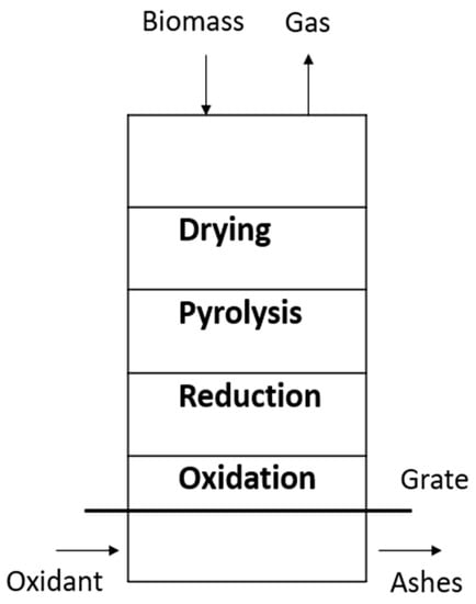
Figure 1.
Fixed bed updraft gasifier.
- Simple and inexpensive;
- Able to cope with biomass with high moisture and high inorganic contents;
- A proven technology.
The high resulting tar content (10 to 20% of tar by weight) that requires intensive cleaning is the main disadvantage of an updraft gasifier. Various researchers have reported on downdraft gasification rather than updraft gasification [7].
Lin et al. [14] investigated the feasibility of rice husk gasification using a fixed bed downdraft gasifier. They started by determining the proximate and ultimate analysis of rice husks. Gas chromatography and infrared spectroscopy were then adopted as the measurement techniques to analyze the temperature and syngas components of their work. As a result, 10 KW of electric power was produced by their system with an approximate 28 kg/h gasification of rice husks. The energy conversion efficiency rate of gasification was about 42.7%; however, the internal combustion engine may convert only 20% of the syngas energy to electricity.
Venkatesh et al. [15] employed different biomass feedstocks, including coconut shells, ground nutshells, sugar cane bagasse, and rice husks in an updraft gasifier. From the experimental study with a 1 h operating time for each feedstock, the temperatures for the zones of combustion, reduction, pyrolysis, and drying were 750 °C, 420 °C, 250 °C, and 180 °C, respectively. They observed that the gas production rate may be promoted by increasing the temperature. Sugar cane bagasse achieved the maximum gas fabrication rate with a gasification efficiency of up to 53.86%, while rice husks represented the lowest efficiency with only 46.96%.
Singh et al. [16] used a downdraft fixed bed gasifier to add steam to a hearth in order to improve gasification efficiency. Using rice husks as the raw fuel, the feeding rate was 16.34 kg/h. The inlet air rate was 40.77 kg/h and 18.77 kg/h of steam was added. By adding steam, water–gas reactions in the gasifier produced an increase in the hydrogen concentration from 18% to 40%, while the gasification efficiency increased from 70% to 80%.
Kihedu et al. [17] utilized an updraft gasifier with a height of 1000 mm in their work. They conducted experiments with air and steam-air in which black pine pellets were adopted as the feedstock. The result showed that syngas with a slightly improved heating value of 4.5 MJ/Nm3 was generated from steam-air gasification in comparison to 4.4 MJ/Nm3 generated by air gasification alone. An improvement in carbon conversion from 84.3% to 91.4% was also found.
Pandey et al. proposed AI models including MISO and MIMO ANNs with a Levenberg–Marquardt backpropagation algorithm to simulate the gasification of municipal solid waste (MSW), and their simulation results matched their experimental data [18]. Mikulandrić et al. compared different modeling approaches for a biomass gasification process and found that an ANN model was able to deal with nonlinear problems where no extensive knowledge regarding the process is needed [19].
In addition, Baruah et al. applied Garson’s equation to calculate the relative importance of the input variables and proposed an artificial neural network model of biomass gasification in fixed bed downdraft gasifiers. The results of this study proved that the model could satisfactorily predict the compositions of four major gas species produced as products (CH4, CO, CO2, and H2) [20].
Puig-Arnavat et al. proposed ANN models of a biomass gasification process in two fluidized bed reactors. One included circulating fluidized bed gasifiers (CFB) and the other included bubbling fluidized bed gasifiers (BFB) [21]. Seven variables were selected as inputs and a backpropagation algorithm with two neurons in the hidden layer was chosen. The results of this architecture matched with the experimental data and a high correlation coefficient was obtained.
George et al. proposed an ANN model using MATLAB for gasification process simulation based on extensive data acquired from experimental investigations. They applied their model to predict the syngas composition from selected biomasses within an operating range [22]. The Levenberg–Marquardt backpropagation algorithm was employed for multi-layer feed-forward neural network training. Satisfactory results with a high regression coefficient (value of R was 0.987) and low mean squared error (value of MSE was 0.71) were reported.
Bahador et al. proposed six AI techniques to model the solubility of CO2 in ionic liquids for capturing CO2 [23]. According to their research, the solubility of CO2 in 1-n-butyl-3-methylimidazolium tetrafluoroborate was estimated using six AI methods, including four ANNs, support vector machines (LS-SVM), and an adaptive neuro-fuzzy interface system (ANFIS). The results showed that the cascade feed-forward neural network had the best performance regarding the solubility of CO2. Table 1 summarizes the key points of the aforementioned studies related to biomass gasification.

Table 1.
Key point of each study in the literature review.
This paper presents an experiment and model of a steam-air biomass gasification process in an updraft gasifier. The experimental data are presented and compared, including temperature profiles, gas compositions, and the LHV. In addition, two nonlinear ANN and GBR models are developed to simulate the biomass gasification process and predict syngas compositions. ANNs are popular models that many researchers have used alongside biomass gasification processes. The GBR model uses a decision tree method that has not been used for biomass gasification before. A notable feature of the GBR is that consecutive corrections are made to minimize the prediction error during the operating process. This seems to be a suitable method for the prediction of biomass gasification, in which limited input parameters are available. The prediction results of both models are compared with experimental data to show the feasibility of AI prediction for rice husk gasification.
2. Methodology
2.1. Experimental Rig and Operating Conditions
In this study, a fixed bed updraft gasifier was employed as shown in Figure 2a. This gasifier was developed by the Clean Power and Green Energy Laboratory of NCHU [24]. Various operating conditions were set up with Taiwanese rice husks as the feedstock.
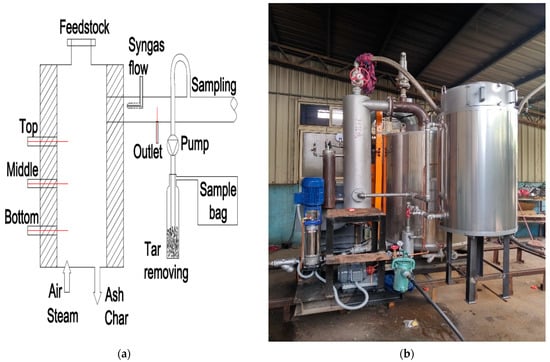
Figure 2.
(a) Model of the gasifier; (b) boiler.
In the beginning, rice husks were burned inside the chamber to raise the temperature to around 700 to 800 °C The feeding rate was kept at 16.8 kg/h. After the completion of the syngas sampling process for air gasification, steam at 160 °C (heated by a boiler, Figure 2b) was added at the bottom of the reactor, thus mixing with air as the gasifying agent. The steam flow rate varied from 0 to 12 kg/h and the air supply was reduced to 43.8 kg/h. The operating conditions for the experimental process are summarized in Table 2.
Table 2.
The operating conditions for the experimental process.
The air and steam flow rates varied in different cases. Pressure and temperature inside the gasifier were recorded and the syngas compositions were analyzed in the final process. Part of the produced syngas was sampled for analysis of the gaseous composition using Agilent’s 6850 Gas Chromatograph device. Tar and water vapor were removed by a cleanup system using filter, condenser, and fridge. The gases that could be measured by the gas chromatograph were hydrogen, nitrogen, carbon monoxide, carbon dioxide, and methane, while the remaining gas was assumed to be oxygen.
2.2. ANNs and GBR Model
This paper adopted the Keras deep learning tool in the form of an application programming interface (API) in Python as a framework to define and train the neural network models. The coding process included preprocessing and the loading of data. Models were defined with a specified number of hidden layers in the neural network and their input and output sizes are included here. The loss function was defined accordingly, while the optimizer and the number of epochs were set to train the neural network and fit the model. An example of the ANN model structure is shown in Figure 3, including three input features, two hidden layers, and one output target. The number of hidden layers and neurons can be adjusted to minimize the error between the input and output data. These adjustments will affect the performance of the model.
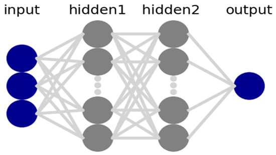
Figure 3.
ANN model structure.
The GBR algorithm used here was based on Friedman’s research [25] and exists in a Python format too. The coding process included preprocessing, the loading of data, defining the model, and fitting the model. The GBR algorithm can combine many weak learning models and create a strong predictive model. It is an ensemble algorithm that can fit boosted decision trees by reaching a minimum error gradient.
Ensembles were constructed from decision tree models where trees were increased one at a time to fix the prediction errors made by previous models. An example of the iteration procedure of the GBR model is illustrated in Figure 4. The process was repeated until decent result quality was obtained. The GBR model is an effective machine learning algorithm as the loss gradient is minimized with its use.

Figure 4.
Iteration procedure of the GBR model.
3. Results
The rice husks were fed at a rate of 16.8 kg/h in this experiment. The proximate and ultimate analyses of rice husks were obtained by Lin et al. [14,26,27,28,29,30] as shown in Table 3. Average values were taken according to figures shown in the table. The following interpretation was carried out with the averaged proximate and ultimate analyses.
Table 3.
Proximate and ultimate analyses of rice husks [14,26,27,28,29,30].
According to the averaged ultimate analysis, the equivalent chemical formula for rice husks can be presented as CH1.52O0.679. The complete combustion formula for a rice husk is given as follow:
CH1.52O0.679 + 1.041(O2 + 3.76N2) → CO2 + 0.76H2O + 3.914N2
The stoichiometric air fuel ratio of a rice husk may be obtained as 5.887 according to Equation (1) and the equivalence ratio was calculated as below:
In the gasifier, the amount of air was not sufficient to oxidize the rice husk completely. The equivalence ratio was always less than 1. At ER = 0.58, the reaction inside the gasifier can be represented as below:
where X represents the amount of syngas that was produced in the gasifier and Y represents the amount of water vapor that has been condensed out of the refrigerator. The steam gasification process incorporated a series of complex reactions as revealed below [26]:
CH1.52O0.679+ 0.604(O2 + 3.76 N2) ≥ X × (a CO + b CO2 + c H2 + d CH4 + e O2 + f N2) + Y H2O + Ash +Tar,
Boudouard reaction:
C + CO2 ⇔ 2CO + 172 kJ/mol
Water–gas (primary) reaction:
C + H2O ⇔ CO + H2 + 131.5 kJ/mol
Methanation reaction:
C + 2H2 ⇔ CH4 − 74.8 kJ/mol
Steam reforming reaction:
CH4 + H2O ⇔ CO + 3H2 + 206 kJ/mol
Water–gas shift reaction:
CO + H2O ⇔ CO2 + H2 − 41 kJ/mol
The temperature variations inside the gasifier were measured at four locations: the top, middle, bottom, and outlet of the gasifier. Typical variations of temperature inside the gasifier are presented in Figure 5. The green arrows represent the timing when the operating condition was changed during the gasification process. Rice husks should be burned with an external fire to start the process. The first green arrow is the completion time of the initial burning of rice husks. After the start period, the temperature at the bottom reached 700 °C. This is the level required to initiate the gasification process.
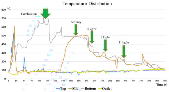
Figure 5.
Temperature distribution of the top, middle, and bottom of the gasifier.
More rice husks were then continuously fed into the hearth of the gasifier. The temperature inside the gasifier dropped immediately as new rice husks covered the old pile. Oxidation reactions occurred and the temperature gradually rose again to reach 600 °C. The process of adding rice husks continued until syngas was produced. The temperature at the bottom varied between 500 °C and 570 °C when oxidation occurred, as shown by the second green arrow. A minor drop in temperature at the lower part was related to the reduction of airflow rate and increase in the steam flow rate. At the third green arrow, 5 kg/h of steam was adjusted and the temperature in the reactor dropped to 300 °C. The last two green arrows denote the the temperature to be around 280 °C for 8 kg/h and not more than 200 °C when steam was added at 11 kg/h. This seems to prove that the temperature at the upper part did not vary significantly.
The syngas was collected after stabilizing the reactor temperature. Figure 6 presents the syngas compositions during the updraft gasification process when only air was used as the gasification agent. Several measurements were made for each gas. The concentrations of each gas are represented by three bars. The blue bars represent the minimum values of the measurements, the grey bars represent the maximum, and the red bars represent averages. On average, the syngas was composed of 5.2% H2, 8.8% CO, 2.1% CH4, and 15.6% CO2.
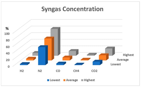
Figure 6.
Syngas compositions during air and steam-air gasification with 0 kg/h of steam.
When steam was added, reactions (5)–(8) may occur. Increments in H2, CO, CH4, and CO2 could then be found. At an 8 kg/h steam rate, the highest concentration of the combustible gas was obtained, but a decrease in combustible gas was observed after the steam flow rate reached 11 kg/h.
Since hydrogen is the most valuable component of syngas, the H2 contents of syngas obtained in the experiments with different operating conditions are therefore shown in Figure 7. The horizontal axis represents the number of a given dataset. A total of 74 sets of data were collected in the experiments. Each dataset is composed of three different operating conditions and five gas compositions. The operating conditions are listed in Table 2 including 11 levels of ER, 4 values of steam flow rate, and 44 levels of bottom-temperature. Without steam addition, the hydrogen content remains low. With steam addition, the hydrogen content rises up as shown in Figure 7.
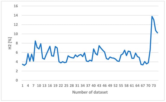
Figure 7.
The H2 content of syngas in different operating conditions.
Adding more steam would not help to produce more syngas because steam is condensed to water inside the bed and results in a lower temperature, which prohibits the reaction from happening. The existence of nitrogen dilutes the produced gas and deteriorates the gas quality. By adding steam, the nitrogen in syngas decreased from 66.2% to 44.5%. The syngas composition is affected by the steam temperature, the ratio of steam to biomass, and the biomass feeding rate, while there is no significant change depending on the size of biomass feedstock [31]. As the feeding rate increased, the contribution of pyrolysis for gas evolution increased. This is because H2 was mainly generated from the char gasification zone and a low H2 concentration was noticed at a low biomass feeding rate.
The lower heating value (LHV) of the raw syngas could be calculated as below:
LHV = QCO × XCO + QH2 × XH2 + QCH4 × XCH4,
The LHVs of each combustible gas are presented in Table 4.
Table 4.
Low heating values of the gases.
The heating values of syngas can be divided into three types: low (4–6 MJ/Nm3), i.e., when using air or steam-air, medium (12–18 MJ/Nm3), i.e., when using oxygen and steam, and high (40 MJ/Nm3), i.e., when using hydrogen and hydrogenation. Rice husks have the lowest heating value for different types of biomass [7]. Table 5 presents the LHVs of syngas as calculated by Equation (9). As the combustible gases increased in the product, the LHVs rose from 2.5 MJ/Nm3 to 5.2 MJ/Nm3. The highest value was recorded at 8 kg/h of steam addition while the lowest was for air alone.
Table 5.
Lower heating values of syngas.
Shackley et al. proposed a biochar gasification system and found that the economic value of the rice husk char (RHC) could vary from USD 9 per ton to USD 15 per ton according to economic assessment. Recycling RHC typically represents an additional income source [32]. According to our experiments, 1 kg of rice may produce about 14.5 MJ of syngas. The heating value of syngas is 2.5 MJ/m3 without the addition of steam. The market value of syngas can be evaluated by the price of domestic natural gas. The retail price of natural gas in Taiwan is 0.35 USD/m3 at the present time. The heating value of natural gas is 32 MJ/m3. It is estimated that 1 kg of rice husk may generate USD 0.15 of syngas.
In Taiwan, rice husks are treated as agriculture waste. It is costly to collect, transport, and burn rice husks in an incinerator. A successful gasification process would be beneficial for farmers.
4. Discussion
In this study, ANNs and GBR models were adopted to simulate the gasification process and predict syngas compositions. A total of 74 sets of data were used in the modeling. These datasets were divided randomly into two subsets, including a training subset (70%) and testing subset (30%). Following this, 51 sets of data were randomly chosen as the training subset while the remaining 23 sets belonged to the testing subset.
The equivalence ratio (ER), bottom-temperature, and steam flow rate independent variables were used as the input features of the model in this study. ER was calculated by Equation (2) with the measured air flow rate. Bottom temperature was obtained by direct measurement with a K-type thermocouple inserted into the hearth. Steam flow rate was controlled with a valve and a flowmeter. The syngas compositions, including H2, CH4, CO, CO2, and N2, were the target of the prediction.
The model performance was examined by using the coefficient of determination or R2. The R2 is a statistical measure that explains the amount of variance between the target values and the predicted results. It was determined by Equation (10), where Pi is the predicted value obtained with the model and Ti is the measured value in experiment. is the average of the predicted value for the whole subset data.
The results of ANNs and GBR models are listed in Table 6. These results include the performances of training subset (51 samples), testing subset (23 samples), and all data (74 samples).
Table 6.
Statistics of the performance of the ANN and GBR models.
The table shows that the regression of the training subset was beneficial for both models. The R2 values varied in the range of 0.89 to 0.94 for the ANN model and 0.96 to 0.99 for the GBR model; however, the R2 values were below the standard for the ANN and model varied in the range of 0.63 to 0.81 for the testing subset. The GBR model was also unsatisfactory, where R2 varied in the range of 0.59 to 0.82.
Since the training data, which accounts for 70% of the total dataset, were selected randomly, it was necessary to conduct a new selection of training data to confirm the effect of the choice of testing data on the model performance. The R2 values of the training subset for the new choice vary in the range of 0.90 to 0.94 for the ANNs model and 0.98 to 0.99 for the GBR model. As a result, the random choice of training data seemed to have a minor effect on the performance of the prediction model.
Figure 8 shows the comparison of H2 predictions with the experimental data. The blue dots scattered on the diagram represent the testing data chosen for both models. The data without blue dots denotes the training subset. The blue dots have been placed on the curve of experimental data to facilitate comparison between the prediction and experimental data. It was revealed that both the ANN and the GBR models, to a great extent, match with the experimental data for the training subset (without blue dots). This is consistent with the results shown in Table 6, in which the R2 for the training data is 0.93 for the ANN model and 0.97 for the GBR model; however, for the testing data represented with blue dots, deviations occurred between the prediction and measured data, especially for the ANN model with the 16th, 18th, 19th, 42nd, 52nd, 54th, 57th, and 65th datasets.
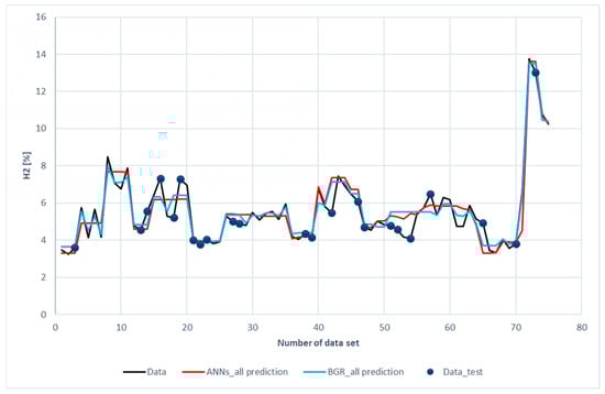
Figure 8.
Comparison of H2 compositions among the experimental data of the ANN and GBR models.
The deviation between the prediction and measured data was two-folded. On the one hand, the input features (ER, bottom-temperature, and steam flow rate) were close, but, on the other hand, the hydrogen compositions were far apart. Measurement uncertainty and a lack of other input features were the reasons for the deviation. In the ANN model, additional L1 and L2 layer weight regulators for the kernel and bias were set to prevent over-fitting. The absolute weight (L1) and the square of its weight (L2) can be used to penalize the model. These values can affect the model loss. Therefore, optimization of L1 and L2 will save the calculation cost. The values of L1 and L2 used in ANNs models are listed in Table 7.
Table 7.
L1 and L2 values.
This explains why the predictions of the ANN model were comparatively straightforward when compared to the GBR model, as shown by the flat red lines of Figure 9. There was no regulator for the GBR model. As a result, the GBR model could fit well with the highest and lowest data and obtain better regression performance than the ANN model.
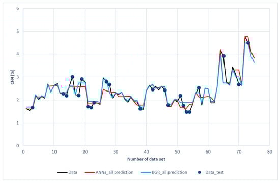
Figure 9.
Comparison of CH4 compositions among the experimental data with the ANN and GBR models.
Figure 9 illustrates a comparison of CH4 prediction with the experimental data. It was revealed that both the ANNs and the GBR models, to a great extent, matched with the experimental data for the training subset. This was consistent with the results shown in Table 6, in which the R2 for the training data was 0.93 for the ANN model and 0.98 for the GBR model. For the testing data, the deviations in the GBR model were less than those of the ANN model. The R2 values in Table 6 also show the same result. The R2 values for the GBR and ANN models were 0.77 and 0.73, respectively. Worth noting that deviations occur in different data of CH4 from those of H2; however, the same cause as in H2 prediction was identified after a closer look at the data. Again, the input features were close to the data but the methane compositions were far apart.
Figure 10 displays a comparison of CO prediction with the experimental data. It is revealed that both the ANN and the GBR models, to a great extent, matched with the experimental data for the training subset, just as in the cases of H2 and CH4. This is consistent with the results shown in Table 6, in which the R2 for the training data was 0.94 for ANN model and 0.99 for the GBR model. For the testing data, deviations in the GBR model were less than those in the ANN model. The R2 values in the GBR model and the ANN model were 0.77 and 0.73, respectively. The same cause as in the H2 and CH4 prediction was identified after a closer look at the data. Again, the input features were close to the data but the carbon monoxide compositions were far apart.
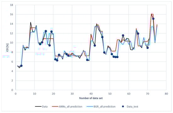
Figure 10.
Comparison of CO compositions among the experimental data with the ANN and GBR models.
Figure 11 and Figure 12 show the comparison of CO2 predictions and N2 predictions with the experimental data of the ANN and GBR models. The same trends for performance are shown in these two figures as those for H2, CH4, and CO. It was revealed that both the ANN and the GBR models, to a great extent, matched with the experimental data for the training subset. For the testing data, the deviations in the GBR model were the same as the ANN model for CO2; however, the ANN model outperformed the GBR model in the case of N2. This is the only case where the ANN model recorded better performance than the GBR model in this study.
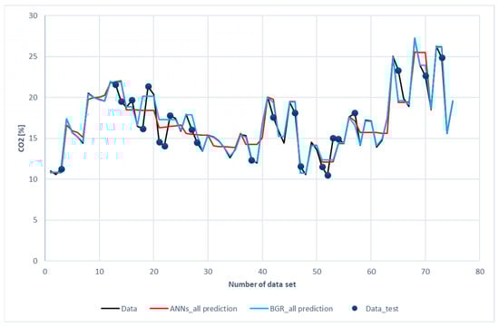
Figure 11.
Comparison of CO2 compositions among the experimental data for the ANN and GBR models.
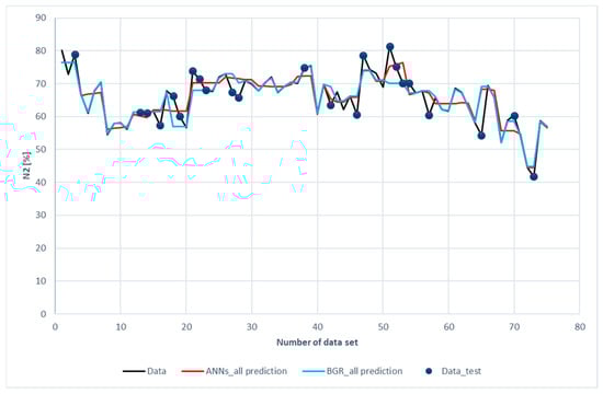
Figure 12.
Comparison of N2 compositions among the experimental data for the ANN and GBR models.
A brief conclusion for the comparison between the experimental data, ANN and GBR models can be drawn: Both the ANN and GBR models have outstanding performance regarding the prediction of the training data. The performances for the testing data were not satisfactory when compared to those of the training data. Nevertheless, the GBR model outperformed the ANN model in most cases.
Figure 13a,b present another comparison for the performance of both models. The results of the prediction were compared with different color curves and scatter plots. A scatter plot is a graph of points that show the relationship between experimental and prediction data. It is a convenient way to present the correlation between two variables. H2 predictions for these two models are shown in Figure 13a. The results of the GBR model (green dots) are closer to the diagonal line than the ANN model. This echoes with the results shown in Figure 8.
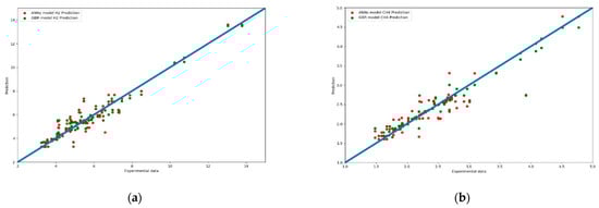
Figure 13.
(a) Scatter plot of the comparison of syngas compositions in H2 prediction between the experiment data for the ANN and GBR model. (b) Scatter plot of the comparison of syngas compositions for CH4 prediction among the experiment data for the ANN and GBR models.
Figure 13b shows a scatter plot of CH4 prediction between the two models. In the intervals of 1.5% to 3.0% (86% of data), the predictions of the GBR model (green dots) were closer to the diagonal line than the ANN model. Some of the ANN model predictions deviated from the diagonal line.
5. Conclusions
In this paper, an experimental study of updraft biomass gasifiers using rice husks was conducted under various conditions. The gasifying agents included pure air and a mixture of steam and air. Rice husks were burned at 700 °C in the beginning and the gasification process started at 500 °C with the addition of pure air. This was then followed by adding more steam to mix with the air. The temperature variations and compositions of syngas were recorded for analysis.
When the ratio of steam to biomass increased, the concentrations of combustible syngas rose. The combustible gases reached their highest value at a steam flow rate of 8 kg/h. An increase in steam flow rate would not enhance the production of syngas. A hydrogen-rich syngas was produced with a low heating value in the range of 2.5 MJ/Nm3 for air and 5.2 MJ/Nm3 for steam-air gasification.
Two AI models, ANN and GBR, were built and used successfully in this study. The compositions of five gases (CO, CO2, H2, CH4, and N2) were predicted. The results showed that the regression of the training subset was beneficial for both models and the effects on the performance of the prediction model by random choice of training data were minor; however, the testing subset deviations were close to the data for the input features, i.e., ER, bottom-temperature, and steam flow rate, while the syngas compositions were far apart.
The performance of the GBR model outperformed the ANN model. The coefficients of determination (R2) for the five gases in the GBR model were higher those in the ANN model. The coefficients of determination (R2) of the ANN model were lower than those of the GBR model. This was caused by the kernel and bias regulators being set in the ANN model. The predictions of the ANN model were more straightforward than those of the GBR model, especially for data that fluctuated. The GBR model could perform fitting well with the highest and lowest data and obtained better regression performance than the ANN model.
The models developed in this paper have provided quite good results to predict compositions of syngas in an updraft gasifier; however, the models have been limited to rice husks only and the operating conditions do not cover all possible scenarios of rice husk gasification. More types of biomass gasification, including wood pellet, wax briquette, and palm kernel shells would be ideal next steps to broaden the applicability of this research.
Author Contributions
Conceptualization, H.-T.W. and J.-H.L.; methodology, H.-T.W. and M.-X.P.; software, H.-T.W.; validation, H.-T.W. and J.-H.L. and M.-X.P.; data curation, M.-X.P.; writing—original draft preparation, H.-T.W.; writing—review and editing, H.-T.W.; supervision, J.-H.L.; All authors have read and agreed to the published version of the manuscript.
Funding
This research received no external funding.
Institutional Review Board Statement
Not applicable.
Informed Consent Statement
Not applicable.
Data Availability Statement
Data is contained within the article.
Conflicts of Interest
The authors declare no conflict of interest.
Nomenclature
| LHV | Lower heating value kJ/Nm3 |
| ER | Equivalence ratio |
| °C | Temperature scale, centigrade |
| X | Mass fraction |
| Y | Mass fraction |
References
- Kannan, N.; Vakeesan, D. Solar energy for future world—A review. Renew. Sustain. Energy Rev. 2016, 62, 1092–1105. [Google Scholar] [CrossRef]
- Blanco, I. The economics of wind energy. Renew. Sustain. Energy Rev. 2009, 13, 1372–1382. [Google Scholar] [CrossRef]
- Tester, J.W.; Anderson, B.J.; Batchelor, A.S.; Blackwell, D.D.; Di Pippo, R.; Drake, E.M.; Veatch, R.W.J. The Future of Geothermal Energy; Massachusetts Institute of Technology: Cambridge, MA, USA, 2006; Volume 358. [Google Scholar]
- Henderson, R. Design, simulation, and testing of a novel hydraulic power take-off system for the Pelamis wave energy converter. Renew. Energy 2006, 31, 271–283. [Google Scholar] [CrossRef]
- Esfandi, S.; Baloochzadeh, S.; Asayesh, M.; Ehyaei, M.A.; Ahmadi, A.; Rabanian, A.A.; Das, B.; Costa, V.A.F.; Davarpanah, A. Energy, Exergy, Economic, and Exergoenvironmental Analyses of a Novel Hybrid System to Produce Electricity, Cooling, and Syngas. Energies 2020, 13, 6453. [Google Scholar] [CrossRef]
- Sikarwar, V.S.; Zhao, M.; Fennell, P.S.; Shah, N.; Anthony, E.J. Progress in biofuel production from gasification. Prog. Energy Combust. Sci. 2017, 61, 189–248. [Google Scholar] [CrossRef]
- Couto, N.; Rouboa, A.; Silva, V.; Monteiro, E.; Bouziane, K. Influence of the Biomass Gasification Processes on the Final Composition of Syngas. Energy Procedia 2013, 36, 596–606. [Google Scholar] [CrossRef]
- Liu, K.; Chunshan, S.; Velu, S. Hydrogen and Syngas Production and Purification Technologies; John Wiley & Sons: Hoboken, NJ, USA, 2010. [Google Scholar]
- Chu-Kuo Hsiao, H.-M.L. Utilization Promotion of Energy and Resource in Organic Agricultural Waste. Master’s Thesis, CYUT, Taichung, Taiwan, 2014. [Google Scholar]
- Bhattacharya, S.; Wu, W. Fluidized bed combustion of rice husk for disposal and energy recovery. Energy Biomass Wastes 1989, 12, 591–601. [Google Scholar]
- Zarei, V.; Nasiri, A. Stabilizing Asmari Formation interlayer shales using water-based mud containing biogenic silica oxide nanoparticles synthesized. J. Nat. Gas Sci. Eng. 2021, 91, 103928. [Google Scholar] [CrossRef]
- Zarei, V.; Mirzaasadi, M.; Davarpanah, A.; Nasiri, A.; Valizadeh, M.; Hosseini, M. Environmental Method for Synthesizing Amorphous Silica Oxide Nanoparticles from a Natural Material. Processes 2021, 9, 334. [Google Scholar] [CrossRef]
- Baruah, D. Modeling of biomass gasification: A review. Renew. Sustain. Energy Rev. 2014, 39, 806–815. [Google Scholar] [CrossRef]
- Lin, K.S.; Wang, H.; Lin, C.-J.; Juch, C.-I. A process development for gasification of rice husk. Fuel Process. Technol. 1998, 55, 185–192. [Google Scholar] [CrossRef]
- Venkatesh, G.; Reddy, P.R.; Kotari, S. Generation of producer gas using coconut shells and sugar cane bagasse in updraft gasifier. Mater. Today Proc. 2017, 4, 9203–9209. [Google Scholar] [CrossRef]
- Singh, A.; Srivastava, N.K.; Yadav, V.; Kumar, D. Thermodynamics Study and Improving Efficiency of Biomass Gasifier. Adv. Res. Electr. Electron. Eng. 2015, 2, 47–51. [Google Scholar]
- Kihedu, J.H.; Yoshiie, R.; Naruse, I. Performance indicators for air and air–steam auto-thermal updraft gasification of biomass in packed bed reactor. Fuel Process. Technol. 2016, 141, 93–98. [Google Scholar] [CrossRef]
- Pandey, D.S.; Das, S.; Pan, I.; Leahy, J.J.; Kwapinski, W. Artificial neural network based modelling approach for municipal solid waste gasification in a fluidized bed reactor. Waste Manag. 2016, 58, 202–213. [Google Scholar] [CrossRef] [PubMed]
- Mikulandrić, R.; Lončar, D.; Böhning, D.; Böhme, R.; Beckmann, M. Artificial neural network modelling approach for a biomass gasification process in fixed bed gasifiers. Energy Convers. Manag. 2014, 87, 1210–1223. [Google Scholar] [CrossRef]
- Baruah, D.; Hazarika, M. Artificial neural network based modeling of biomass gasification in fixed bed downdraft gasifiers. Biomass Bioenergy 2017, 98, 264–271. [Google Scholar] [CrossRef]
- Puig-Arnavat, M.; Hernández-Pérez, J.A.; Bruno, J.C.; Coronas, A. Artificial neural network models for biomass gasification in fluidized bed gasifiers. Biomass Bioenergy 2013, 49, 279–289. [Google Scholar] [CrossRef]
- George, J.; Arun, P.; Muraleedharan, C. Assessment of producer gas composition in air gasification of biomass using artificial neural network model. Int. J. Hydrogen Energy 2018, 43, 9558–9568. [Google Scholar] [CrossRef]
- Daryayehsalameh, B.; Nabavi, M.; Vaferi, B. Modeling of CO2 capture ability of [Bmim][BF4] ionic liquid using connectionist smart paradigms. Environ. Technol. Innov. 2021, 22, 101484. [Google Scholar] [CrossRef]
- Liao, J.-H. Energy Analysis of Gasification with Different Biomass in a Fixed Bed Gasifier. Master’s Thesis, NCHU, Taichung, Taiwan, 2020. [Google Scholar]
- Friedman, J.H. Greedy function approximation: A gradient boosting machine. Ann. Stat. 2001, 29, 1189–1232. [Google Scholar] [CrossRef]
- Fang, M.; Yang, L.; Chen, G.; Shi, Z.; Luo, Z.; Cen, K. Experimental study on rice husk combustion in a circulating fluidized bed. Fuel Process. Technol. 2004, 85, 1273–1282. [Google Scholar] [CrossRef]
- Lo, K.-C.; Chyang, C.S.; Lo, H.H. A Study of Rice Husks Combustion in a Vortexing Fluidized Bed Combustor. In Asian Pacific Confederation of Chemical Engineering Congress Program and Abstracts; The Society of Chemical Engineers: Tokyo, Japan, 2004. [Google Scholar]
- Madhiyanon, T.; Sathitruangsak, P.; Soponronnarit, S. Combustion characteristics of rice-husk in a short-combustion-chamber fluid-ized-bed combustor (SFBC). Appl. Therm. Eng. 2010, 30, 347–353. [Google Scholar] [CrossRef]
- Duan, F.; Chyang, C.; Chin, Y.; Tso, J. Pollutant emission characteristics of rice husk combustion in a vortexing fluidized bed in-cinerator. J. Environ. Sci. 2013, 25, 335–339. [Google Scholar] [CrossRef]
- Kuprianov, V.I.; Kaewklum, R.; Chakritthakul, S. Effects of operating conditions and fuel properties on emission performance and combustion efficiency of a swirling fluidized-bed combustor fired with a biomass fuel. Energy 2011, 36, 2038–2048. [Google Scholar] [CrossRef]
- Umeki, K.; Namioka, T.; Yoshikawa, K. Analysis of an updraft biomass gasifier with high temperature steam using a numerical model. Appl. Energy 2012, 90, 38–45. [Google Scholar] [CrossRef]
- Shackley, S.; Carter, S.; Knowles, T.; Middelink, E.; Haefele, S.; Sohi, S.; Cross, A.; Haszeldine, S. Sustainable gasification–biochar systems? A case-study of rice-husk gasification in Cambodia, Part I: Context, chemical properties, environmental and health and safety issues. Energy Policy 2012, 42, 49–58. [Google Scholar] [CrossRef]


Publisher’s Note: MDPI stays neutral with regard to jurisdictional claims in published maps and institutional affiliations. |
© 2021 by the authors. Licensee MDPI, Basel, Switzerland. This article is an open access article distributed under the terms and conditions of the Creative Commons Attribution (CC BY) license (https://creativecommons.org/licenses/by/4.0/).