Weather Data Mixing Models for Day-Ahead PV Forecasting in Small-Scale PV Plants

Abstract

As a large number of small-scale PV plants have been deployed in distribution systems, generation forecasting of such plants has recently been gaining interest. Because the PV power mainly depends on weather conditions, it is important to accurately collect weather data for relevant PV sites to enhance PV forecasting accuracy. However, small-scale PV plants do not often have their own measuring apparatus to get historical weather data, so they have used weather datasets from relatively nearby weather data centers (WDCs). Therefore, these small-scale PV plants have difficulty delivering robust and reliable forecasting accuracy because of inappropriate predicted weather data from a distance. In this paper, two weather data mixing models are proposed: (a) inverse distance weighting (IDW), and (b) inverse correlation weighting (ICW). These models acquire adequate mixed weather data for the day-ahead generation forecasting for small-scale PV plants. Furthermore, the mixed weather data are collected using the geographic distance between the PV site and WDCs, or correlation between the PV generation and weather variables from nearby WDCs. Interestingly, the proposed ICW model outperforms when WDCs are located distant from the PV plants, whereas IDW performs well with the closer WDCs. The forecasting performance of the proposed mixing models was compared with those of the existing weather data collection methods.

1. Introduction

Different distributed energy sources, such as photovoltaic (PV) power generation, wind power generation, and energy storage devices, are the essential components of a modern smart grid. Among them, PV power generation is sharply increasing worldwide because of its convenient installation, the increasing demand for clean energy, and to meet other priorities set by the different countries [1]. To maintain huge clean energy demand, large-scale and small-scale PV plants require to be installed in various geographical regions [2]. Large-scale PV plants usually have their meteorological offices to record historical weather data for short-term PV forecasting (STPF) operations. However, small-scale PV plants are generally less economical and may not have the facilities for weather data collection. For their STPF operation, a weather dataset is often used from the closest weather data center (WDC), where the distance and meteorological weather conditions are often offset.

To date, many approaches have been proposed for STPF, such that they are entirely dependent on implementing the predicted weather conditions [3]. Overall, these approaches can be categorized into (a) statistical, (b) learning-based, and (c) hybrid. Statistical approaches, such as the ordinary least square model [4], vector auto-regression model [4], gradient boosting [4], sine cosine algorithm [5], extreme learning machine [5,6], and empirical mode decomposition [6], perform predictions using only historical PV data. These models assume that the PV series emulates the behavior of a nonstationary time series, and the predicted PV generation is simply based on historical observations and seasonality modeling [7]. Learning-based methods are gaining more interest because of their simple implementation and valid forecasting accuracy. These include both machine and deep learning algorithms, such as support vector regression [8], back-propagation neural network (BPNN) [9,10,11], long short-term memory (LSTM) networks [12,13,14], and convolutional neural networks (CNNs) [15]. BPNN, LSTM, and CNN are state-of-the-art deep learning algorithms that facilitate convenient implementation in the PV forecasting sector. However, they present higher forecasting accuracy only when the training set of each model comprises either a sufficient amount of data or homogenous input data. Because many small-scale PV plants have recently been installed, the collection of a large amount of historical PV data is a major issue that requires to be resolved. Consequently, the recent STPFs follow a hybrid mechanism to obtain better PV forecasting outputs.

Hybrid PV forecasting methods mainly focus on either specific or similar day identification [16,17,18,19,20,21,22]. Euclidean distance (ED)-based optimization [16], statistical analysis software (SPSS) [17], discrete wavelet transformation (DWT) [19], radial basis function [20], and wavelet packet distribution (WPD) [21] are the statistical techniques used for the determination of a specific type of day from historical days. Moreover, learning-based clustering techniques, such as support vector machines (SVMs) [19], k-nearest neighbors (k-NN) [17], and self-organizing map classification [14,22], are the major classification approaches that extract similar weather days. A strong similar day detection (SDD) method that deals with different impacts of weather variables for collecting homogenous PV generation profiles was developed [14]. The common aim of these hybrid techniques is to determine a similar day from the historical data for better forecasting outputs.

Based on the literature review, many PV forecasting approaches use the predicted weather data that are either obtained from the same location or from the closest WDC. The dependency on the closest WDC is one of the major reasons for encountering higher forecasting errors, particularly in small-scale PV plants. To overcome such issues, exploiting the maximum weather information is necessary for all accessible WDCs. These WDCs may be deployed in various geographical regions within a certain distance. In [23], passing cloud issues were introduced and resolved based on the geographical region for multi-plant PV forecasting. Wind speed is used to estimate the spatial correlation for modeling PV plants in new locations [24]. However, unusual geographical structures and different weather conditions may occur within this distance. In fact, the procedure for collecting weather data might capture inadequate observations because of the distance. With distance, cloud movement and windy activities vary, typically in hilly or mountainous areas. The optimum tilted angle of the solar panel also has a significant impact on PV generation within a city area [25]. In addition, elevation and humidity often affect PV generation, and they differ from place to place [26]. Consequently, a novel methodology needs to be developed to overcome this problem while collecting weather data from distant WDCs for small-scale PV plants.

The objective of this study was to investigate the feasibility of attaining a higher forecasting accuracy for small-scale PV plants by collecting a more reliable weather dataset from all the accessible WDCs. In this study, two weather data mixing models were proposed to solve the distance problem while collecting weather data from WDCs. These mixing models include the (1) inverse distance weighting (IDW) model, and (2) inverse correlation weighting (ICW) model, and they incorporate a computation of the mixing of weather data from all the reachable WDCs. The proposed IDW model collects the potential weightage weather data from all the WDCs. This weightage is calculated by inverting the distance between the PV plant and WDC. The proposed ICW model computes the weightage for all the WDCs that is similar to the IDW model, where ensemble correlation is used instead of distance. Two existing weather calibration methods are used for comparison: (1) raw data from the closest WDC, and (2) average weather data. Although the averaged weather data utilizes the weather data from all the accessible WDCs, it is considered to be a conventional method.

After the weather data were collected based on all the methods, the existing SDD-based day-ahead PV forecasting technique [14] was used for comparison. The output of the SDD provides four new PV series for the training process. Each new PV series is assumed to be homogenous and passed through the LSTM-based forecasting network. In this study, four PV plants were used to compare the performances that were deployed in different geographical regions. Because the distance impacts the weather data collection, only accessible WDCs are selected within the confined distance. The simulation results verify that the proposed IDW and ICW models collect useful weather data and enhance the forecasting output for all the PV plants. These models are particularly significant for all types of new and old small-scale PV plants that are installed and deployed in remote and diverse geographical regions.

The rest of the paper is organized as follows. Section 2 discusses the issues in the existing weather data collection for the STPF technique. Section 3 explains the proposed weather data mixing models, along with the existing SDD-based PV forecasting algorithm. Section 4 discusses the PV plants and weather data, hyperparameter tuning, and simulation results. Finally, Section 5 concludes the paper.

2. Weather Data Collection Problem

Despite the impact of various factors, including the formation of clouds from dense water vapors, the passing clouds and windy activities are considered trivial for PV fluctuations. These issues play a key role when there is a significant distance between the PV plants and WDCs. WDCs are mostly located in and around the city area because of higher public activities and cost factors. Because the earth surface and weather conditions are spatially variable, these factors are easily blocked or diverted. In fact, the collection of weather data from the closest WDC is unsuitable for the forecasting task. If hills and mountains are between the WDCs and the PV plant, the collected weather data are considered to be inadequate. Figure 1a,b show the conventional and proposed STPF approaches for the small-scale PV plant, respectively. In Figure 1a, the weather data are directly used from the closest WDC for the STPF task. In Figure 1b, weather data from four accessible WDCs were mixed for better STPF results of the small-scale PV plants.

Although the amount of solar radiation is the most important parameter for PV prediction, it is not directly available from agencies [26]. Other weather parameters, such as the cloud cover, sunshine hours, humidity, and wind, also provide significant information for PV generation. For example, the differences in cloud movement over PV plants mainly create uncertain PV generation output. Because the impact of these parameters varies between places, the direct selection of the closest WDC for weather data collection is problematic. In addition, other accessible WDCs might be an option to exploit the useful information. Therefore, considering the weather data from the accessible WDCs could be effective for STPF operation in small-scale PV plants.

The larger the distance between the PV plant and WDC, the higher the probability of obtaining inferior weather data. Therefore, the collected weather dataset cannot effectively address the latent relationship between PV generation and weather parameters. Figure 2 depicts the average correlation measure between the generation of PV power and the cloud cover of each of the four WDCs. The nearest data center, WDC 1, and the most remote data center, WDC 4, are located at 6.01 km and 40.9 km away from the PV plant, respectively. In Figure 2, WDC 1 exhibits a better correlation measure only in the months of August and October. However, WDC 2 and WDC 3 demonstrate better results in April and December, respectively. In addition, WDC 4 presents comparable results with respect to WDC 1, for April, August, and December.

From Figure 2, none of the WDCs explicitly reveal a better correlation measurement, although cloud cover is the paramount weather parameter in PV forecasting. In addition to the cloud cover uncertainty, the distance has a significant impact on the relationship between the weather parameters and PV generation. Furthermore, the correlation values of the same WDC varied monthly. It is obvious that there is a problem in accepting weather data only from the closest WDC. Therefore, exploiting meaningful information from all the accessible weather data is one of the major approaches considered to enhance the reliability of the collected weather data. To obtain sufficient information, the inherent problem related to distance and weather data computation needs to be acknowledged.

3. PV Forecasting Based on Proposed Weather Data Mixing Models

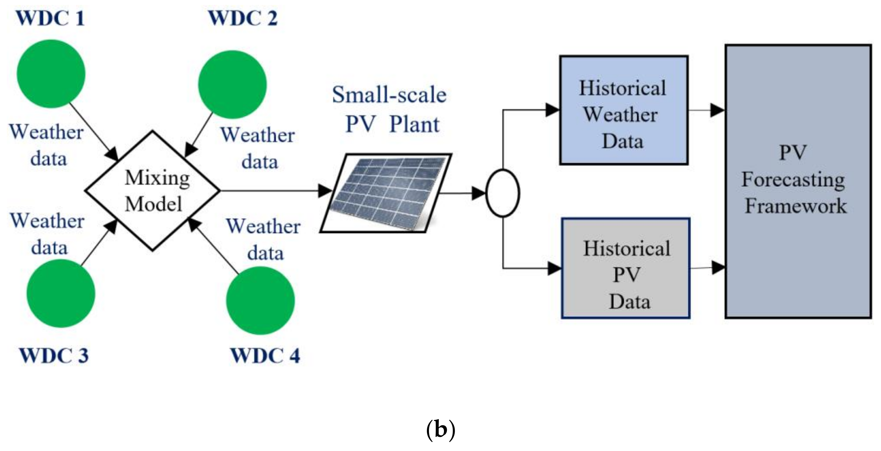
3.1. Weather Data Mixing Models

Let the historical PV generation of any small-scale PV plant $P$, be expressed as follows:

$$P=\left[p_1,p_2,p_3,\dots .,p_d,\dots ..p_D\right]$$

(1)

where $p_d=\left[p_{d,1},p_{d,2},p_{d,3}\dots p_{d,t},\dots p_{d,T}\right]$ represents the PV generation profile of day $d$ with PV generation at time t, and D represents the number of days in the historical data. In addition, the plant may have $M$ different nearby WDCs located at distances $\left[{\lambda }_1,{\lambda }_2,\dots {\lambda }_m\dots {\lambda }_M\right]$. The plant collects weather data, $\left[W_d^1,W_d^2,\dots .W_d^m\dots W_d^M\right]$, from $M$ different WDCs for each day. Using n different weather variables $W_d^m=\left[w_{d,1}^m,w_{d,2}^m, \dots .w_{d,n}^m\dots w_{d,N}^m\right]$, each WDC performs daily weather observations. Each weather variable, $n$, has the daily observations, $w_d^{m,n}=\left[w_{d,1}^{m,n},w_{d,2}^{m,n},w_{d, 3}^{m,n},\dots .w_{d, t}^{m,n},\dots ..w_{d, T}^{m,n}\right],$ where $w_{d, t}^{m,n}$ represents the numerical weather value at time $t$ for WDC m.

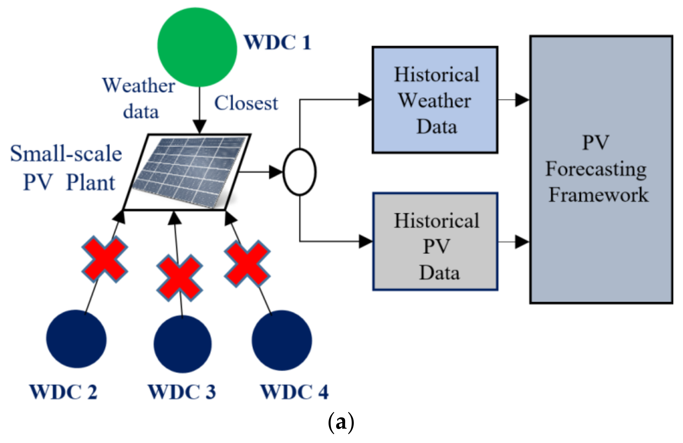
3.1.1. Raw Weather Data from the Closest WDC

The collection of raw weather data from the closest WDC is an existing method of weather data collection for small-scale PV plants. The reliability of the collected weather data depends on the distance between the PV plant and the closest WDC. The closest WDC model collects the weather data, $W_d^{CL}$, for day $d$, based on the shortest distance. The minimum distance, ${\lambda }_m$, is directly calculated from ${\lambda }_1,{\lambda }_2,\dots ,{\lambda }_m,\dots ,{\lambda }_M$, that are the distances between the PV plant and $M$ different WDCs. Based on the minimum index m, the weather data of the shortest distant WDC $m$, were directly used for $W_d^{CL}$.

3.1.2. Averaged Weather Data

Another existing approach through which the weather data can be easily calculated for a small-scale PV plant is the averaging of all the accessible weather data. The average weather data, $W_d^{AVG}$, for day $d$ was calculated as follows:

$$W_d^{AVG}=\left(W_d^1+W_d^2+\cdots +W_d^m+\cdots +W_d^M\right)/M\hspace{1em}\forall d$$

(2)

Both $W_d^{CL}$ and $W_d^{AVG}$ collect the adequate weather data when all the available WDCs are deployed within a few kilometers. The region needs to be either plain or it may even feature small hills. However, the geographical structure of the earth, such as hills and mountains, may have a higher altitude that usually alters the movement of clouds, windy phenomena, and humidity observation. Consequently, the collected weather data consist of a large amount of distraction and do not account for the significant improvement in the forecasting performance.

3.1.3. Inverse Distance Weighting (IDW) Model

The proposed IDW model is a deterministic approach in spatial interpolation that is comparatively fast and straightforward [27]. Major applications of the IDW equation are particularly found in the distance-based interpolation applications, such as wireless sensor networks [28], geographic information systems (GIS) [29], and computer science [30]. It facilitates the collection of valid weather data for a small-scale PV plant from a distance. This method assigns a weight for each WDC based on the inverse of the distance. A higher weight implies a closer distance between the PV plant and WDC and vice versa. The IDW model that accesses the weather data, $W_d^{IDW}$, for day $d$ is defined as:

$$W_d^{IDW}=\frac{{\sum }_{m=1}^M{W}_d^m/{\lambda }_m}{{\sum }_{m=1}^{M}1/{\lambda }_m}.$$

(3)

Because an increase in distance outturns a decrease in inverse distance, the closest WDC has a higher impact on $W_d^{IDW}$ than the remote WDCs. Although $W_d^{IDW}$ captures meaningful weather information based on the distance, it does not account for the inherent relationship between PV generation and weather variables. In addition, when all the WDCs are located at a far distance, the collected $W_d^{IDW}$ demonstrates a weak performance. Based on this weather data, the varying impact between PV generation and weather parameters is difficult to acknowledge.

3.1.4. Inverse Correlation Weighting (ICW) Model

The proposed ICW model assumes that the meteorological weather parameters have latent information for weather data calibration. The considerably more important latent information may vary among the weather data of each WDC. This varying impact can be captured through the correlation measures between the PV generation data and weather data.

Because this study considers multiple WDCs for a single PV plant, each WDC has a different correlation measure between their historical weather data and PV generation data. For any WDC $m$, the proposed ICW model evaluates the correlation measure ${\rho }_{d, n}^m$, of weather variable n, for day $d$ that is given by:

$${\rho }_d^{m,n}=\frac{{\sum }_{t=1}^T\left(p_{d,t}-{\overline{p}}_d\right)\left(W_{d,t}^{m,n}-{\overline{W}}_d^{m,n}\right)}{\sqrt{{{\displaystyle \sum }}_{t=1}^T{\left(p_{d,t}-{\overline{p}}_d\right)}^2{{\displaystyle \sum }}_{t=1}^T{\left(W_{d,t}^{m,n}-{\overline{W}}_d^{m,n}\right)}^2}},$$

(4)

where ${\overline{p}}_d$ is the daily average of PV generation for day $d$; ${\overline{W}}_{d, n}^m$ is the daily average value of weather variable $n$ for day $d$. Equation (4) shows the diversity in correlation values that are calculated between the PV generation data and weather data, based on the weather variable n. The correlation values ranged from −1 to 1. The entire correlation information from all the weather variables is an ensemble, as given by:

$${\rho }_d^m={\displaystyle \sum }_{n=1}^N{\rho }_d^{m,n},$$

(5)

where ${\rho }_d^m$ is the ensemble correlation measure of WDC m for day d. Unlike the distance, ${\rho }_d^m$ varies only slightly among $M$-WDCs. Because the impact of the various factors related to the weather changes day by day, the ensemble correlation measure also changes. To overcome such deep and disparate complexity in correlation information, the inverse value of $\left|{\rho }_d^m\right|$ is used for mixing the weather data for day $d$ that is given by:

$$W_d^{ICW}=\frac{{\sum }_{m=1}^M{W}_d^m/\left|{\rho }_d^m\right|}{{\sum }_{m=1}^{M}1/\left|{\rho }_d^m\right|} .$$

(6)

3.2. Similar Day Detection (SDD)

A robust SDD method was previously proposed by the authors’ research group [14]. The SDD was developed based on a clustering algorithm [31]. Initially, employing this SDD method, the historical PV generation profiles were classified into $K$-different PV groups. Thereafter, each weather dataset from each model is separately passed to the SDD to detect similar day group k, for the next day.

Based on the identified similar day group k, the weather data belonging to similar weather group k, are detected from the passed weather dataset. The weather dataset is initially normalized because each weather variable has a different range. Within similar weather group k, the numerical weather predicted value $w_{k,d}^n$ of each weather variable $n$ for day d is determined. Each $w_{k,d}^n$ of weather variable n within a similar weather group k has an average numerical weather predicted value ${\overline{w}}_k^n$. Each weather variable n shows a deviation measure among the average predicted numerical weather values. This deviation $r_{ }^n$ is the difference between the maximum and minimum average numerical weather predicted values ${\overline{w}}_k^n$, as follows:

$$r_{}^n=\underset{k}{\max }\left({\overline{w}}_k^n\right)-\underset{k}{\min }\left({\overline{w}}_k^n\right)\mathrm{for}\mathrm{all}n$$

(7)

where n represents the weather variable and k represents the similar weather group k.

There is a vast literature on the impact of weather variables on PV generation [7,17,32]. Although there is a complex relationship between them, the input weather variables were directly categorized into two parts: primary weather variables (PWVs) and secondary weather variables (SWVs) [14]. PWVs are highly correlated weather variables for PV generation. However, SWVs are useful for acquiring only homogenous PV generation profiles within an identified group, k.

Weather variables with a higher deviation, rⁿ, are selected as PWVs by defining a threshold $\alpha$ [14]. Within a similar weather group k, the deviation $s_{k }^n$ is the difference between the maximum and minimum numerical weather predicted values $w_{k,d}^n$, as follows:

$$s_{k }^n=\underset{d}{\max }\left(w_{k,d}^n\right)-\underset{d}{\min }\left(w_{k,d}^n\right)$$

(8)

where n represents the weather variable, and $w_{k,d}^n$ is the numerically predicted value in the similar weather group k for day d. The weather variables that have a higher SWV deviation $\left(s_k^n\right)$ than the SWV threshold $\beta$, are selected as SWVs [14].

In order to generate new homogenous PV series $P_{in}$ for the next day PV forecasting, the PWV variables that have higher deviation $r^n$ are used to identify the similar weather group k as follows:

$$\underset{k}{\mathrm{argmin}}{\displaystyle \sum }_{n\in pwv}\left|{\overline{w}}_k^n-w_{D+1}^n\right|,$$

(9)

where $w_{D+1}^n$ is the numerical predicted weather value of the weather variable $n$ for the next day $D+1$. In order to select more similar days from the similar weather group k, SWV similarity index ${\varphi }_{k,d}$ for day d within a weather group k is calculated as follows:

$${\varphi }_{k,d}={\displaystyle \sum }_{n\in swv}\left|w_{k,d}^n-w_{D+1}^n\right|$$

(10)

The lower value of ${\varphi }_{k,d}$ explores the more similar days that are detected by defining the constant threshold $\gamma$ [14]. With these days, corresponding PV generation profiles are collected in $P_{in}$. Consequently, $P_{in}$ considerably solves the homogenous data requirement issues in PV forecasting.

3.3. Proposed Weather Data Mixing Model-Based PV Forecasting Framework

The raw weather data from the closest WDC, average weather data, and mixed weather data obtained based on the two proposed models might be dissimilar, although the same SDD is applied. Consequently, four different homogenous PV series, $P_{in}^{CL}$, $P_{in}^{AVG}$, $P_{in}^{IDW}$, and $P_{in}^{ICW}$, were obtained from the SDD. These series contain different numbers of homogenous PV generation profiles, although the selected PWVs and SWVs are the same. Each SDD output series is passed to the LSTM-based forecasting framework for the next-day PV prediction and comparison of results. Figure 3 illustrates the overall flow chart of the proposed weather data mixing model-based day-head PV forecasting framework for small-scale PV plants.

LSTM networks are found in many applications of PV forecasting [12,14], residential load forecasting [33], natural language processing [34], and speech recognition [35]. This network has improved PV forecasting accuracy when the input PV series contains numerous repetitive daily PV generation profiles. The selection of an inadequate PV generation profile in the training series may increase the forecasting errors, and the forecasting error is unavoidable.

The common goal of all SDD output series is to predict the day-ahead PV generation profile. Because these series behave similar to a time series, with only a difference in the length of the training data, a similar LSTM-based training model is developed for all the input PV series. The temporal dependencies (long- or short-term) between previous and current PV generation are effectively established using several components of the LSTM structure, such as internal memory cell, forget gate, input gate, and output gate. To learn complex patterns in PV generation data, these LSTM components are composed of corresponding activation functions. The LSTM training model is tracked, checked, and updated based on the sum of the mean square error (MSE) using the back-propagated gradient-based algorithm. Let ${\widehat{p}}_D$ and $p_D$ represent the predicted and actual PV generation profiles for day D at time step t. The developed objective function that minimizes the MSE can be written as:

$$\underset{\theta }{argmin}\Vert {\widehat{p}}_D-p_D{\Vert }_F^2,$$

(11)

where $\Vert ·{\Vert }_F$ is the Frobenius norm, and $\theta$ represents the modeling parameter of the LSTM network. This parameter comprises various weights and biases that are repeatedly updated during the training process.

4. Simulation Results and Discussion

To evaluate the forecasting performance of the all-weather data collection method, two performance evaluation metrics were used: the mean absolute percentage error (MAPE) and root mean square error (RMSE). The day-ahead forecasting error, in terms of MAPE and RMSE, was measured using the following equation:

$$MAPE=\frac{1}{T}{\displaystyle \sum }_{t=1}^T\frac{\left|p_{D+1, t}-{\widehat{p}}_{d+1,t}\right|}{P_{capacity}}\times 100\%,$$

(12)

$$RMSE=\sqrt{\frac{{\sum }_{t=1}^T{\left(p_{D+1, t}-{\widehat{p}}_{d+1,t}\right)}^2}{T}} ,$$

(13)

where $p_{D+1, t}$, and ${\widehat{p}}_{D+1,t}$ are the actual and predicted PV generation at time step $t$, respectively, and $P_{capacity}$ is the total installed PV capacity.

4.1. Data Description

To evaluate the proposed methodologies, the historical PV series were collected from four PV plants among twenty PV plants located in South Korea. The duration of the evaluation was one year, commencing from January 2018 and ending in December 2018. Weather parameters, such as average temperature, wind speed, wind direction, humidity, sunshine hours, cloud cover, atmospheric pressure, and rain amount, were used as weather variables. The average temperature, wind speed, humidity, atmospheric pressure, and rain amount are measured using a general scale of measurement. In addition, sunshine hour, cloud cover, and wind direction are measured in terms of percentile. Each observation of the weather variables is a ground observation that is performed at a fixed and same observation time. These parameters were successfully implemented in a previous study [14,25]. The Meteorological Agency’s Open Weather Portal Office of South Korea performs weather observations using weather variables throughout the country and publishes via websites. Because South Korea is a country that mainly comprises mountains, several small valleys, and many narrow coastal plain regions, these tested PV plants are selected assuming that the maximum area will be covered.

Table 1. Information of PV plants with corresponding distant weather points.

PV Plant	PV Capacity (kW)	Location	Weather Data Center (WDC)	Distance
PV Plant 1	1000	Samcheok	1	41.7
			2	35.3
			3	46.01
PV Plant 2	40	Yeoungwol	1	6.01
			2	12.05
			3	28.8
			4	40.9
PV Plant 3	1000	Incheon	1	5.7
			2	26.6
PV Plant 4	300	Hadong	1	26.3
			2	32.8
			3	40.9

shows the information about all the tested PV plants with the corresponding WDCs located at a certain distance. PV plants 1, 2, and 4 are located in remote hilly areas, whereas PV plant 3 is located in the city area. The selected plants do not have their individual meteorological data center for daily weather evaluation. The distance between PV plants and nearby WDC is limited to 50 km, which is the line-of-sight distance in mobile communication.

In Table 1, only PV plant 2 had four WDCs that were accessible within a radius of 50 km. As the proposed ICW model deals with correlative information, the collected mixed weather data from this model and weather data from the four WDCs were used for correlation comparison. Figure 4 depicts the correlation comparison results between the ICW model and the four WDCs for April, August, October, and December. In Figure 4, the proposed ICW model shows a noteworthy improvement in the correlation measure that confirms the importance of the weather-mixing model.

4.2. Hyperparameter Tuning

The proposed weather-mixing method, the SDD method, and LSTM-based forecasting models were developed and tested using the Python programming language. The SDD and LSTM-based forecasting models use the Keras and TensorFlow library [34,36], along with the basic Python library. The proposed PV forecasting approach is simulated in a Windows operating environment using an i7–600 CPU at 3.40 GHz and 16 GB of installed RAM.

Table 2. Hyperparameters for LSTM-based forecasting framework.

Hyperparameters	LSTM Network
Hidden layers	2
Nodes per layer	24, 12
Activation function	sigmoid, tanh
No. of epochs (iteration)	300
Optimizer	RMS-prop
Loss function	MES
Metrics function	accuracy
Batch size	32
Validation set	10%

shows the optimum hyperparameter tuning for the LSTM-based forecasting model, inspired by [33,37].

Hidden layers, loss function, and optimizer are the common hyperparameters of the deep learning methodology, where an increase in more than three hidden layers still does not imply a higher forecasting performance in time series analysis [33]. For the proposed LSTM network, two hidden layers with 24 and 12 nodes were used in the first and second layers, respectively. These layers are composed of a nonlinear activation function (sigmoid and tanh). The model was trained by using resilient back-propagation (RMSprop) optimizer, which has better convergence over long short-term dependencies. The training process was maintained within 300 iterations because the input PV series were small and homogenous. Mean squared error (MSE) was set as an evaluation metric, and batch size was set at 32 to obtain a proper gradient for the optimum convergence. For each day-ahead forecasting operation, each input dataset was divided into a testing set (1 day), validating set (10% days), and training set (remaining days).

4.3. Day-Ahead PV Forecasting Output

Figure 5 depicts the actual and day-ahead PV forecasting outputs from the proposed models and existing methods of PV plants 1, 2, 3, and 4 during a randomly selected week.

Table 3. One-week average forecasting performance results.

	Average MAPE (%)				Average RMSE (kW)
PV Plant	Closest	Average	IDW	ICW	Closest	Average	IDW	ICW
PV plant 1	13.92	11.40	11.52	11.64	195.03	161.93	165.86	167.09
PV plant 2	9.41	9.16	8.57	8.81	5.20	4.79	4.26	4.65
PV plant 3	6.70	6.35	6.41	6.25	92.43	91.18	90.37	89.69
PV plant 4	13.12	12.79	11.89	10.48	58.01	54.87	49.05	44.01

shows the forecasting performance results in terms of the average MAPE and RMSE for the selected week.

For the selected week, the ICW model showed better forecasting output with PV plants 3 and 4. The averaged weather data and IDW model demonstrated precise performance results with PV plants 1 and 2, respectively. The PV plants 2 and 3 have the closest WDC at a distance of 6.01 km and 5.7 km, respectively. In these PV plants, the difference in the average MAPE results varied slightly within 1%. However, the nearest WDC for PV plants 1 and 4 was located at least 25 km away. These PV plants demonstrate above 1.5% variation in the MAPE results. The difference in MAPE results may be due to the distance between the PV plant and the nearby WDCs. The proposed ICW model shows a significant MAPE result, greater than 1.41%, as compared with the IDW model (the second-best performer) in PV plant 4. Both the proposed IDW and ICW models showed better forecasting accuracy compared to the existing methods. This explains both the distance- and correlation-based proposed models, which are particularly significant and useful for the mixing of weather data from all the accessible WDCs.

4.4. Seasonal Evaluation

The weather dataset shows entangled activities when the seasons are changed. In [10], the weather dataset was decomposed into spring, summer, autumn, and winter to acquire a better forecasting output. However, the splitting process for weather data may cancel the inherent consistency of the weather dataset. To maintain regularity in the weather data, this study used prior 120-day windowing for each day-ahead PV prediction. To perform seasonal evaluation, the proposed method selects four arbitrary weeks from each season. Figure 6 shows box plot results of the overall MAPE computed based on the proposed models and the existing methods for PV plants 1, 2, 3, and 4.

Table 4. Seasonal average MAPE and RMSE results of the tested PV plants, obtained using proposed models and existing methods.

		MAPE (%)				RMSE (kWh)
		Closest	Average	IDW	ICW	Closest	Average	IDW	ICW
PV Plant 1	Spring	10.21	10.83	10.89	10.36	140.19	155.56	157.71	145.71
	Summer	14.37	11.45	11.80	11.44	222.47	167.05	172.43	170.62
	Autumn	10.19	11.95	11.86	10.15	143.18	192.73	194.96	144.45
	Winter	11.56	11.32	11.09	10.55	167.77	161.21	185.11	148.51
	Average	11.58	11.39	11.41	10.62	168.40	169.14	177.55	152.32
PV Plant 2	Spring	9.72	9.50	9.25	9.32	4.90	5.01	4.85	4.77
	Summer	9.94	9.01	9.49	9.27	5.53	5.20	5.49	5.08
	Autumn	11.13	10.48	10.51	10.03	5.89	5.36	5.14	5.17
	Winter	9.93	10.11	9.93	9.80	5.60	5.58	5.54	5.49
	Average	10.18	9.77	9.60	9.60	5.48	5.28	5.25	5.12
PV Plant 3	Spring	10.37	11.69	10.61	10.92	160.40	166.81	161.61	168.57
	Summer	9.39	9.98	9.46	9.46	145.41	149.52	145.65	146.23
	Autumn	11.48	11.37	10.77	11.77	165.48	164.31	144.86	167.88
	Winter	12.55	12.28	12.03	12.32	171.67	174.70	180.51	176.13
	Average	10.94	11.33	10.71	11.12	160.74	163.83	158.19	164.70
PV Plant 4	Spring	11.62	10.56	10.72	9.91	53.59	48.80	48.09	45.61
	Summer	10.86	10.59	10.51	10.38	47.56	46.38	44.90	44.08
	Autumn	10.02	9.17	9.04	8.82	40.44	40.61	37.79	37.78
	Winter	10.29	10.72	10.95	10.60	46.49	48.64	49.37	47.89
	Average	10.69	10.26	10.30	9.92	47.02	46.10	45.53	43.84

shows seasonal average MAPE and RMSE results from the proposed models and existing methods of the PV plants 1, 2, 3, and 4. For PV plants 1 and 4, the proposed ICW model shows improvements above 0.8% and 0.3%, respectively, in terms of forecasting MAPE compared with the average weather data (the second-best performer). In the case of PV plant 3, the IDW model shows improved forecasting MAPE and RMSE results, above 0.2% and 2.58 kWh, respectively. Because PV plant 3 has one WDC located at a distance of 5.27 km, the IDW model provides improved RMSE results compared with the correlation-based ICW model.

PV plant 2 has four WDCs, and the closest WDC is situated at a distance of 6.01 km. In this PV plant, the proposed ICW model outperforms all the proposed distance-based models by more than 0.13 kW for the average RMSE results. Similarly, in terms of the MAPE results, both the ICW and IDW models are comparable in each season of the year. This highlights that the proposed ICW and IDW models have an improved weather data collection ability from the nearby WDCs.

5. Conclusions

In this paper, two weather data mixing models were proposed to collect suitable weather data for day-ahead PV forecasting in small-scale PV plants. These mixing models collect mixed weather data from all the accessible WDCs within a defined distance. Among the four PV plants tested, two PV plants that had the closest WDC at least 25 km away exhibited better performances compared with the proposed ICW model. In these plants, the impact of the distance from the source of weather data was significantly reduced. In addition, the other proposed IDW model showed a higher PV forecasting accuracy in the other two PV plants, which have the nearest WDC located within 6 km. However, the raw weather data obtained by using the closest WDC (a conventional weather data collection method for the STPF task) did not lead to better PV forecasting accuracy in all the tested small-scale PV plants. This highlights that the proposed models enhanced the forecasting accuracy for small-scale PV plants, even when these plants were installed and deployed in remote areas from the WDCs. In the future, the day-by-day selection procedure of the mixing model will be developed that increases the forecasting performance for the small-scale PV plants.

References

1. Kim, H.; Park, H. PV Waste Management at the Crossroads of Circular Economy and Energy Transition: The Case of South Korea. Sustainability 2018, 10, 3565. [Google Scholar] [CrossRef] [Green Version]
2. Jamal, T.; Urmee, T.; Shafiullah, G.M.; Carter, C. Technical Challenges of PV Deployment into Remote Australian Electricity Networks: A Review. Renew. Sustain. Energy Rev. 2017, 77, 1309–1325. [Google Scholar] [CrossRef]
3. Das, U.K.; Tey, K.S.; Seyedmahmoudian, M.; Mekhilef, S.; Idris, M.Y.I.; Van Deventer, W.; Horan, B.; Stojcevski, A. Forecasting of Photovoltaic Power Generation and Model Optimization: A review. Renew. Sustain. Energy Rev. 2018, 81, 912–928. [Google Scholar] [CrossRef]
4. Bessa, R.J.; Trindade, A.; Miranda, V. Spatial Temporal Solar Power Forecasting for Smart Grids. IEEE Trans. Ind. Inform. 2014, 3203, 1–10. [Google Scholar] [CrossRef]
5. Wan, C.; Lin, J.; Song, Y.; Xu, Z.; Yang, G. Probabilistic Forecasting of Photovoltaic Generation: An Efficient Statistical Approach. IEEE Trans. Power Syst. 2017, 32, 2471–2472. [Google Scholar] [CrossRef] [Green Version]
6. Behera, M.K.; Nayak, N. A Comparative Study on Short Term PV Forecasting Using Decomposition Based Optimized Extreme Learning Machine Learning Algorithm. Eng. Sci. Technol. Int. J. 2019, 23, 156–167. [Google Scholar] [CrossRef]
7. Han, Y.; Wang, N.; Ma, M.; Zhou, H.; Dai, S.; Zhu, H. A PV Interval Forecasting Based on Seasonal Model and Nonparametric Estimation Algorithm. Sol. Energy 2019, 184, 515–526. [Google Scholar] [CrossRef]
8. Alfadda, A.; Adhikari, R.; Kuzlu, M.; Rahman, S. Hour-Ahead Solar PV Forecasting Using SVR Based Approach. In Proceedings of the 2017 IEEE Power & Energy Society Innovative Smart Grid Technologies Conference (ISGT), Washington, DC, USA, 23–26 April 2017; pp. 1–5. [Google Scholar]
9. Li, Z.; Rahman, S.M.; Vega, R.; Dong, B. A Hierarchical Approach Using Machine Learning Methods in Solar Photovoltaic Energy Production Forecasting. Energies 2016, 9, 55. [Google Scholar] [CrossRef] [Green Version]
10. Hu, Y.; Lian, W.; Dai, S.; Zhu, H. A Seasonal Model Using Optimized Multi-Layer Neural Networks to Forecast Power Outputs of PV Plants. Energies 2018, 11, 326. [Google Scholar] [CrossRef] [Green Version]
11. Huang, C.; Cao, L.; Peng, N.; Li, S.; Zhang, J.; Wang, L.; Luo, X.; Wang, J. Day-Ahead Forecasting of Hourly Photovoltaic Power Based on Robust Multilayer Perceptron. Sustainability 2018, 10, 4863. [Google Scholar] [CrossRef] [Green Version]
12. Jung, Y.; Jung, J.; Kim, B.; Han, S. Long Short-Term Memory Recurrent Neural Network for Modelling Temporal Patterns in Long-Term Power Forecasting for Solar PV Facilitates: Case Study of South Korea. J. Clean. Prod. 2020, 250, 119476. [Google Scholar] [CrossRef]
13. Lee, D.; Kim, K. Recurrent Neural Network-Based Hourly Prediction of Photovoltaic Power Output Using Meteorological Information. Energies 2019, 12, 215. [Google Scholar] [CrossRef] [Green Version]
14. Acharya, S.K.; Wi, Y.-M.; Lee, J. Day-Ahead Forecasting for Small-Scale Photovoltaic Power Based on Similar Day Detection with Selective Weather Variables. Electronics 2020, 9, 1117. [Google Scholar] [CrossRef]
15. Aprillia, H.; Yang, H.-T.; Huang, C.-M. Short-Term Photovoltaic Power Forecasting Using a Convolutional Neural Network–Salp Swarm Algorithm. Energies 2020, 13, 1879. [Google Scholar] [CrossRef]
16. Zhang, Y.; Beaudin, M.; Taheri, R.; Zareipour, H.; Wood, D. Day-Ahead Power Output Forecasting for Small-Scale Solar Photovoltaic Electricity Generators. IEEE Trans. Smart Grids 2015, 6, 2253–2262. [Google Scholar] [CrossRef]
17. Cheng, K.; Guo, L.M.; Zafar, M.T. Application of Clustering Analysis in the Prediction of Photovoltaic Power Generation Based on Neural Network. IOP Conf. Ser. Earth Environ. Sci. 2017, 93, 012024. [Google Scholar] [CrossRef]
18. Wang, F.; Zhen, Z.; Wang, B.; Mi, Z. Comparative Study on KNN and SVM Based Weather Classification Models for Day Ahead Short-Term Solar PV Forecasting. Appl. Sci. 2018, 8, 28. [Google Scholar] [CrossRef] [Green Version]
19. Nazaripouya, H.; Wang, B.; Wang, Y.; Chu, P.; Pota, H.R.; Gadh, R. Univariate Time Series Prediction of Solar Power Using a Hybrid Wavelet-ARMA-NARX Prediction Method. In Proceedings of the 2016 IEEE/PES Transmission and Distribution Conference and Exposition (T&D), Dallas, TX, USA, 3–5 May 2016; pp. 1–5. [Google Scholar]
20. Lu, H.J.; Chang, G.W. A Hybrid Approach for Day-ahead Forecast of PV Generation. Int. Fed. Autom. Control. Pap. Online 2018, 51, 634–638. [Google Scholar] [CrossRef]
21. Li, P.; Zhou, K.; Lu, X.; Yang, S. A Hybrid Deep Learning Model for Short-Term PV Forecasting. Appl. Energy 2019, 259, 114216. [Google Scholar] [CrossRef]
22. Yang, H.T.; Huang, C.M.; Huang, Y.C.; Pai, Y.S. A Weather-Based Hybrid Method for 1-day Ahead Hourly Forecasting of PV Output. IEEE Trans. Sustain. Energy 2014, 5, 917–926. [Google Scholar] [CrossRef]
23. Jeong, J.; Kim, H. Multi-Plant Photovoltaic Forecasting Exploiting Space-Time Convolutional Neural Network. Energies 2019, 12, 4490. [Google Scholar] [CrossRef] [Green Version]
24. Ekström, J.; Koivisto, M.; Mellin, I.; Millar, R.J.; Lehtonen, M. A Statistical Model for Hourly Large-Scale Wind and Photovoltaic Generation in New Locations. IEEE Trans. Sustain. Energy 2017, 8, 1383–1393. [Google Scholar] [CrossRef] [Green Version]
25. Kim, G.Y.; Han, D.S.; Lee, Z. Solar Panel Tilt Angle Optimization Using Machine Learning Model: A Case Study of Daegu City, South Korea. Energies 2020, 13, 529. [Google Scholar] [CrossRef] [Green Version]
26. Kim, S.-G.; Jung, J.-Y.; Kyu Sim, M. A Two-Step Approach to Solar Power Generation Prediction Based on Weather Data Using Machine Learning. Sustainability 2019, 11, 1501. [Google Scholar] [CrossRef] [Green Version]
27. Lu, G.Y.; Wong, D.W. An Adaptive Inverse-distance Weighting Spatial Interpolation Technique. Comput. Geosci. 2008, 34, 1044–1055. [Google Scholar] [CrossRef]
28. Shuai, M.; Xie, K.; Chen, G.; Ma, X.; Song, G. A Kalman Filter Based Approach for Outlier Detection in Sensor Networks. In Proceedings of the 2008 International Conference on Computer Science and Software Engineering, Hubei, China, 12–14 December 2008; pp. 154–157. [Google Scholar]
29. Bhattacharjee, S.; Mitra, P.; Ghosh, S.K. Spatial Interpolation to Predict Missing Attributes in GIS Using Semantic Kriging. IEEE Trans. Geosci. Remote Sens. 2014, 52, 4771–4780. [Google Scholar] [CrossRef]
30. Wang, Z.; Xin, J.; Yang, H.; Tian, S.; Yu, G. Distributed and Weighted Extreme Learning Machine for Imbalanced Big Data Learning. Tsinghua Sci. Technol. 2017, 22, 160–173. [Google Scholar] [CrossRef]
31. Kohonen, T. Essentials of the Self-organizing Map. Neural Netw. 2013, 37, 52–65. [Google Scholar] [CrossRef] [PubMed]
32. Alskar, T.; Dev, S.; Visser, L.; Hossari, M.; Sark, V.W. A Systematic Analysis of Meteorological Variables for PV Output Power Estimation. Renew. Energy 2020, 153, 12–22. [Google Scholar] [CrossRef]
33. Acharya, S.K.; Wi, Y.-M.; Lee, J. Short-Term Load Forecasting for a Single Household Based on Convolution Neural Networks Using Data Augmentation. Energies 2019, 12, 3560. [Google Scholar] [CrossRef] [Green Version]
34. Pattanayek, S. Pro Deep Learning with TensorFlow: A Mathematical Approach to Advanced Artificial Intelligence in Python, 1st ed.; Apress: New York, NY, USA, 2017; pp. 223–251. [Google Scholar]
35. Yang, L.; Li, Y.; Wang, J.; Tang, Z. Post Text Processing of Chinese Speech Recognition Based on Bidirectional LSTM Networks and CRF. Electronics 2019, 8, 1248. [Google Scholar] [CrossRef] [Green Version]
36. Pedregosa, F.; Varoquax, G.; Gramfort, A. Scikit-learn: Machine Learning in Python. J. Mach. Learn. Res. 2011, 12, 2825–2830. [Google Scholar]
37. Ozaki, Y.; Yano, M.; Onishi, O. Effective Hyper-Parameter Optimization using Nelder–Mead Method in Deep Learning. PSJ Trans. Comput. Vis. Appl. 2017, 9, 20–25. [Google Scholar] [CrossRef] [Green Version]
Figure 1. STPF of a small-scale PV plant: (a) conventional method to collect weather data from the closest WDC, (b) proposed mixing model to collect mixed weather data from the four WDCs.
Energies 14 02998 g001aEnergies 14 02998 g001b
Figure 2. Monthly average correlation between the PV generation data and cloud cover data from the four nearby WDCs: (a) April, (b) August, (c) October, (d) December.
Energies 14 02998 g002
Figure 3. Overall flow chart of the proposed weather data mixing model-based PV forecasting method for small-scale PV plants.
Energies 14 02998 g003
Figure 4. Correlation comparison results between the proposed ICW model and corresponding four WDCs: (a) April, (b) August, (c) October, and (d) December.
Energies 14 02998 g004
Figure 5. Actual and day-ahead PV forecasting output, obtained based on the proposed models and existing methods for the randomly selected week: (a) PV plant 1, (b) PV plant 2, (c) PV plant 3, (d) PV plant 4.
Energies 14 02998 g005
Figure 6. Box plot results of the overall MAPE results based on the proposed models and existing methods: (a) PV plant 1, (b) PV plant 2, (c) PV plant 3, (d) PV plant 4.
Energies 14 02998 g006