Novel Features and PRPD Image Denoising Method for Improved Single-Source Partial Discharges Classification in On-Line Hydro-Generators

Abstract

In this paper, a novel image denoising algorithm and novel input features are proposed. The algorithm is applied to phase-resolved partial discharge (PRPD) diagrams with a single dominant partial discharge (PD) source, preparing them for automatic artificial-intelligence-based classification. It was designed to mitigate several sources of distortions often observed in PRPDs obtained from fully operational hydroelectric generators. The capabilities of the denoising algorithm are the automatic removal of sparse noise and the suppression of non-dominant discharges, including those due to crosstalk. The input features are functions of PD distributions along amplitude and phase, which are calculated in a novel way to mitigate random effects inherent to PD measurements. The impact of the proposed contributions was statistically evaluated and compared to classification performance obtained using formerly published approaches. Higher recognition rates and reduced variances were obtained using the proposed methods, statistically outperforming autonomous classification techniques seen in earlier works. The values of the algorithm’s internal parameters are also validated by comparing the recognition performance obtained with different parameter combinations. All typical PD sources described in hydro-generators PD standards are considered and can be automatically detected.

1. Introduction

Insulation electrical breakdown is the most common cause of failure in hydro-generators [1]. It is a result of insulation aging due to electrical, mechanical and thermal stresses [2,3]. Local electrical discharges that occur in deteriorated portions of electrical insulation without promoting short circuits are named partial discharges (PDs) [4]. On-line PD monitoring has been the most used technique to evaluate the stator insulation condition [4,5,6], because partial discharges are a key symptom of the insulation degradation mechanisms in course [3].

Each type of insulation defect, when subjected to a high electric field, supports sources of partial discharges with specific characteristics [7,8]. PD recognition is the important task of analyzing such characteristics to estimate the underlying source. This knowledge aids in planning appropriate condition-based maintenance measures, because each defect type generates discharges with particular degradation rates and critical levels [7]. Frequently, PD source diagnosis is performed by human experts [9], which are expensive and time-consuming [5]. Therefore, the development of automatic PD identification expert systems is an important step towards the adoption of PD monitoring at a large scale [9].

PD recognition has been a prolific field of research. In earlier works, several techniques for signal denoising, feature extraction and pattern classification were proposed [10]. Among recent works related to rotating machines, Guzmán et al. [11] compared the performance of support vector machines and artificial neural networks (ANNs) for the recognition of three PD sources. Time domain signals were noise filtered with wavelets, and statistical features were extracted. The method was tested in artificial PD models and in a stator coil. High recognition rates were obtained. However, since that methodology was validated in laboratory conditions, the lower levels of noise and ambiguity result in overestimated rates of correct pattern classification in comparison to the case of on-line hydro-generators. This issue also applies to most papers in the literature [12,13]; few works use data from fully operational generators. In [14], a methodology for PD classification in medium voltage motors based on fractal features is presented. A given pattern sample is classified by comparing its features to reference features obtained from several copies of phase-resolved partial discharge (PRPD) patterns from standards [8]. In terms of drawbacks, the methodology does not recognize all PD types (corona is ignored), and its performance was not statistically evaluated.

Effective PD denoising also plays a key role in source recognition, as the excessive levels of noise in power systems pose great difficulties to the correct detection and interpretation of PD signals [5]. State-of-the-art PD denoising techniques rely on wavelet transforms, which preserve both the time and frequency contents of the signal. Promising results have been reported with this approach [15,16]. However, this method operates on time-domain PD signals, which may not be available in situations with storage constraints due to the high sampling rates and long acquisition time windows required. Frequently, PRPD samples are available because they are compact statistical representations of measurements that are widely used for PD recognition [7]. In those cases, developing and applying image processing algorithms to PRPDs may be the best (or the only) alternative to noise filtering. In the literature, [17,18,19] are apparently the only papers proposing image denoising for PDs. However, only laboratory experiments were conducted in [17,18], and the denoising methodologies of the three works were not statistically evaluated for many samples. Moreover, in [17], the choice of mother wavelet function and cut-off thresholds, which greatly influence filtering results, are left open. It should be noted that many modern commercial acquisition systems also perform PD denoising. However, image-based algorithms remain useful when such systems are not accessible, or when time-domain signals are not available for the previously mentioned reasons.

In our previous paper [20], a single-source PD recognition methodology using neural networks in hydro-generator stator windings was proposed. It seemed to be the first work to statistically evaluate the recognition methodology with on-line measurements in several hydro-generators. However, it does not consider all the typical PD types described in IEC 60034-27-2 [8], and its recognition results can be improved by employing, for example, better feature extraction and PD denoising schemes.

In this article, we propose enhancements to the PD recognition methodology of our previous work [20] in order to achieve higher recognition rates. Those enhancements are a novel image-based PD denoising algorithm for single-source patterns, and novel input features. The PD denoising algorithm is applied directly to PRPD pattern samples, which are treated as images. Its capabilities are the removal of low-density PD regions and of non-dominant PD clouds due to crosstalk (cross-coupling between phases), which are types of noise and interference observed in on-line hydro-generators. To the best of our knowledge, it is the first denoising technique to explicitly handle the issue of crosstalk, which greatly hinders PD classification. The proposed denoising algorithm expects the input pattern sample to be contaminated with heavy noise and other interfering signals, such as those from crosstalk. Using only the information encoded in the PRPD image, the denoising results in a new PRPD containing only the discharges characterizing the dominant PD source, removing as much noise as possible while preserving features of the dominant PD source.

The denoising method alone is not sufficient to significantly improve the results of [20], because it is not compatible with the input features used in that work. The features of [20] are PD projections onto amplitude and phase that mainly account for the high-quantity low-amplitude partial discharges, which frequently contain heavy noise not related to the underlying PD source. Since the denoising method tends to remove higher-amplitude PDs, its results exert little influence on the features of [20] and hence on classification rates. To prevent this issue, we also propose in this study a novel input feature that is more sensitive to the changes produced by denoising. The proposed features are functions of amplitude and phase PD distributions that are influenced more evenly by the partial discharges of different amplitude levels.

The contributions of this study are the following: (i) proposal of novel input features combined with an improved PRPD image denoising algorithm; (ii) consideration of all typical PD sources described in standards; and (iii) achievement of recognition rates numerically comparable to other studies, but obtained in this work under much less restricted circumstances: on-line PD measurements in fully operational hydro-generators.

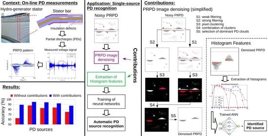
2. Difficulties Affecting PD Pattern Recognition

PD activity is influenced by several factors, leading to great variability in the detected signals [21]. This makes PD recognition a challenging task. The issues for recognition are broadly related to noise and interference, inherent physical phenomena and inappropriate measurement practices. As a result, the signal of interest might become undetectable or ambiguous among different PD sources.

The intense levels of noise and interferences in power systems are the main obstacle for the reliable measurement and classification of partial discharges [5]. The main sources of interference are white noise, random pulses from machine operation or external sources and crosstalk (cross-coupling between phases). In addition to mixing together with PD signals, noise may be misidentified as PD or mask discharges below a certain magnitude. In this context, a number of noise suppression techniques have been proposed, which hold the ultimate goal of enhancing the monitoring system’s sensitivity to partial discharges. In this work, noise is suppressed by applying a novel image processing algorithm to the PRPD pattern sample.

Partial discharge pulses are non-Markovian stochastic phenomena with great statistical variability [21]. Propagation effects are another issue. From the discharge site, PD pulses are subjected to several electromagnetic phenomena (attenuation, reflections etc), such that its shape, amplitude and rise time change significantly along the propagation path [21,22]. For PD recognition, robust expert systems must be designed in order to cope with these inherent physical phenomena. This explains why PD identification is primarily approached with statistical and artificial intelligence (AI) techniques [21].

During measurement, the coupling circuit’s frequency response strongly affects the detected signals, especially in terms of amplitude [7]. An inappropriate selection of frequency range also reduces sensitivity to certain PD types, as discharges from different sources occupy specific bandwidths [7].

3. Review of the Single-Source PD Recognition Methodology Previously Developed by the Authors

It is convenient to briefly review the single-source PD recognition methodology of [20], as it is later used for validating the contributions (improved image denoising and novel input features) of this paper.

The acquisition system used in [20] and in this work is called Instrumentation for Monitoring and Analysis of Partial Discharges (IMA-DP) [23]. Digital high-pass filters are applied to separate the 60 Hz AC voltage from high frequency PD signals. IMA-DP builds PRPD maps relating the amplitude and quantity of PD pulse peaks detected during acquisition as a function of the phase angle of the AC cycle. Amplitude and phase ranges are divided into 256 equal windows each, resulting in a 256 × 256 PRPD. Once PRPDs are formed, time-domain signals are discarded to minimize storage burden.

Sparse PDs are suppressed by applying a simple pixel submatrix technique to the PRPDs. Let the neighborhood of a given pixel be defined as the 5 × 5 submatrix centered in it. The method consists of removing pixels (counts set to zero) that are the only non-zero PD count in their respective neighborhoods.

From the filtered PRPDs, features based on the projection of normalized PD counts onto the amplitude and phase axes are extracted. The counts in the PRPD sample are normalized by the maximum PD count, resulting, in a general case, in a $m\times n$ normalized matrix M. The projections onto the positive ($P_{\mathrm{a}}^{+}$) and negative ($P_{\mathrm{a}}^{-}$) amplitudes are the row-wise sum of normalized PD counts in each polarity. Mathematically:

$$\left\{\begin{array}{c}{P}_{\mathrm{a}}^{+}\left(i\right)=\sum _{j=1}^{n}M(i,j)\hfill \\ P_{\mathrm{a}}^{-}\left(i\right)=\sum _{j=1}^{n}M(i+\raisebox{1ex}{$m$}\!\left/ \!\raisebox{-1ex}{$2$}\right.,j)\hfill \end{array}\right.,i\in \{1,2,\cdots ,\raisebox{1ex}{$m$}\!\left/ \!\raisebox{-1ex}{$2$}\right.\}.$$

(1)

Projections onto the phase are the column-wise sum of normalized PD counts in the positive ($P_{\mathrm{ph}}^{+}$) and negative ($P_{\mathrm{ph}}^{-}$) polarities:

$$\left\{\begin{array}{c}{P}_{\mathrm{ph}}^{+}\left(j\right)=\sum _{i=1}^{m/2}M(i,j)\hfill \\ P_{\mathrm{ph}}^{-}\left(j\right)=\sum _{i=1}^{m/2}M(i+\raisebox{1ex}{$m$}\!\left/ \!\raisebox{-1ex}{$2$}\right.,j)\hfill \end{array}\right.,j\in \{1,2,\cdots ,n\}.$$

(2)

In each pattern, the highest-amplitude positive and negative PDs lie at amplitudes $A_{\mathrm{H}}^{+}$ and $A_{\mathrm{H}}^{-}$, respectively. In order to remove the effect of variable amplitude ranges across PRPD images, 64 equidistant points were used for interpolating $P_{\mathrm{a}}^{+}$ and $P_{\mathrm{a}}^{-}$ within the amplitude range $[-max(A_{\mathrm{H}}^{+},A_{\mathrm{H}}^{-}),$$max(A_{\mathrm{H}}^{+},A_{\mathrm{H}}^{-})]$. In addition, 64 points were used for interpolating each of the phase projections over the entire AC phase cycle. The four interpolated functions were concatenated to form a 256-element feature vector, which characterize each PRPD pattern. As an example, Figure 1 illustrates the projection features of a given PRPD.

The extracted features were used to train feedforward ANNs with the scaled conjugate gradient backpropagation algorithm (SCG) [24]. ANNs are trained in order to mitigate the undesired effects of the random variables involved: topology (number of neurons and hidden layers), data partitioning and initial weights. The best topology is not known in advance, and is usually determined by experimentation [25]. A particular distribution of the data forming the training, validation and test sets may yield biased estimates of neural network performances on unseen data [25]. Initial weights are random parameters that act as the starting points of deterministic gradient-based algorithms (including SCG), thereby completely determining the result of training for a fixed combination of data and ANN topology.

This way, several partitions of the data were considered by means of 4-fold cross-validation (CV) [25], repeated 10 times. A CV partition is a selection of two folds to form the training set, one for validation and the other for testing. In each repetition of CV, the composition of folds is changed with a new random distribution of samples. Several ANN topologies are also considered. For each data partition, 50 ANNs of different initial weights (defined randomly) were trained for every topology. In simulations, the internal random number generator is re-initialized before every repetition of CV for increased randomness.

All ANNs have 256 inputs (same length of the feature vector), a hyperbolic tangent activation function in hidden layers and a softmax function in the output layer. There is one output neuron for each PD source.

4. Data Sets Obtained from On-Line Hydro-Generators

The data sets used in this work are composed of on-line PD measurements performed in hydro-generators at Tucuruí (Figure 2a) and Coaracy Nunes (Figure 2b) power plants, both located in Northern Brazil. All generators are air-cooled, with mica-epoxy insulation type. Generators at Tucuruí are rated 13.8 kV/350 MVA, and the ones at Coaracy Nunes are rated 13.2 kV/24 MVA. PD signals were measured by means of electrical method using the circuit depicted in Figure 3a. The employed sensors were capacitive couplers, installed close to several stator windings of the hydro-generators. Figure 3b shows the acquisition setup, which was used during the on-site measurement of Figure 3c. Signals were sampled and digitized with oscilloscope NI USB-5133 (50 MHz bandwidth; 100 MS/s sampling rate; 8-bit resolution).

The first data set considered in this work was the one used in our previous paper [20], composed of 568 single-source PRPDs. A human expert labeled those patterns among five of the typical stator winding PD sources (classes) described in IEC 60034-27-2 [8]: internal void (InV); slot discharge; corona at the field grading junction; surface tracking; and gap discharges. The specialist labeled the PD source of each sample based on work experience, symmetry between positive and negative PDs and cloud shape. If there are multiple PD clouds in a given PRPD, the dominant PD source is defined as the one associated to the PD clouds with the highest number of pulses. In physical terms, those clouds likely correspond to the PD source that is closest to the sensor. The small distance cause PD pulses to suffer little attenuation and distortion effects on their propagation path from the discharge site to the detector. PRPD samples considered dubious even by the expert were not included in the data set.

A second database (named “extended”) containing PRPDs of all typical PD sources was considered, which is described in IEC 60034-27-2 [8], including internal delamination (InD) and delamination between conductor and insulation (DCI), which are absent in the data set of [20]. There is also less severe class imbalance in the extended database, mainly because of a reduced number of gap discharge samples.

Among the considered sources of partial discharges, the ones most threatening to rotating machines are internal delamination, slot discharges and delamination between conductors and insulation [26].

Note that while forming the databases, the measured PRPDs were carefully analyzed by a specialist with extensive work experience and good knowledge of the generators involved. Based on the expert’s judgement, only PRPDs containing a single PD source were selected to compose the databases of this paper. Moreover, the samples of the databases have been measured for almost a decade. During this period, several samples apparently containing a single PD source were collected, which would be harder to obtain in a short interval of measurements.

The input features used in the work [20] (Equations (1) and (2)) differentiate among most of these classes, but are not able to discriminate between slot and corona and between InV and InD. The PRPD shape, which is the main difference between those sources [8], is often not clearly triangular or rounded, as seen in Figure 4a,b. Those ambiguities are not resolved by the features. Moreover, slot and corona sources are known to present similar pattern characteristics [7]. Therefore, these pairs were merged into two classes (InV/InD and slot/corona) in this paper.

Approximately 60% of the samples in the extended data set are of well-defined patterns (Figure 5), similar to those shown in [8]. The remaining PRPDs are affected by disturbances that hinder PD recognition. Those samples have been more affected by the issues described in Section 2, which are expected to occur due to acquisition in the generator under fully operational conditions [5]. Figure 4c–f show the main types of disturbances affecting the PRPDs of the database: intense noise and crosstalk. The possible sources of intense noise (as seen in Figure 4) may be the detection of other PDs occurring sufficiently close to the sensor, and disturbances in the hydro-generator itself or in nearby equipment such as sparking, arcing, maneuvers in the power system and the action of switching devices [4,8].

5. Proposed Techniques for PRPD Denoising and Feature Extraction

5.1. Preliminary Considerations

In this section, enhancements to the PD recognition methodology of [20] are presented in order to increase classification rates. This goal is achieved by using a modified version of the PD recognition methodology of [20], with different noise filtering and feature extraction stages. The overall PD recognition methodology proposed in this work is illustrated in Figure 6.

PRPD pattern samples are treated as images: PRPDs contain the amplitude and phase of PDs, which are mapped by rows and columns of PRPD images (see, for example, the corona pattern of Figure 5e). Thus, noise filtering is performed with the proposed PRPD image denoising algorithm, and the extracted features are histograms. The filtering technique was designed to be robust to sample pattern variations introduced by the many disturbances found in on-line measurements (Section 2; Figure 4). The two techniques described are the contributions of this work: the PRPD image denoising algorithm is explained in Section 5.2, and the histogram features are described in Section 5.3.

Regarding the terminology used, noise gap (Figure 4a) refers to the PD-absent horizontal zone around zero amplitude. Noise gaps are present because IMA-DP, similarly to other PD measurement systems, does not record the occurrence of PDs with absolute amplitude below a certain trigger level during measurements, for noise suppression purposes. Care was taken during measurements such that all samples in the database have noise gaps of similar width in pixels. PD clouds adjacent to the noise gap are named ANGPD clouds (adjacent to noise gap partial discharges), while others are called N-ANGPD clouds (non-adjacent to noise gap partial discharges), as seen in Figure 4d,f. Amplitude noise refers to spurious low-amplitude PDs uniformly distributed along a section or all the phase cycle (Figure 4c). PDs termed higher or lower are those with higher or lower absolute amplitude relative to others in a given PRPD map.

It is worth mentioning that the terms ANGPD and N-ANGPD describe PDs based solely on their location in the PRPD map, with no relation whatsoever to their underlying physical nature. These terms were chosen to reflect the algorithm’s point of view: PDs are treated as pixels of an image.

5.2. The Proposed PRPD Image Denoising Algorithm

The proposed PRPD denoising methodology is outlined in Figure 7. An input PRPD is subjected to two independent filtering paths. The first path—the sequence of grid filtering, ANGPD phase delimiting and removal of non-dominant ANGPDs—aims at extracting the pair of dominant ANGPD clouds (one positive and one negative). The path’s first step, grid filtering, removes spurious discharges surrounding ANGPD clouds, without distorting the latter. Valid N-ANGPDs of lower density may be removed in this process, especially surface tracking clouds. Those “lost” N-ANGPD discharges are recovered by denoising the input PRPD with the second path, composed of the pixel submatrix technique [20], a lower intensity filtering that removes very sparse noise that may be connecting different N-ANGPD clouds. Once the outputs of the two filtering paths are obtained, their discharges are grouped into different clusters. Certain ANGPD and N-ANGPD clusters from both outputs are then combined in a temporary sample. By analyzing the temporary sample’s ANGPD clusters, it is determined whether the dominant PD source of the input pattern is of ANGPD or N-ANGPD type. The final filtered PRPD is formed by the temporary sample’s PDs that only belong to clusters of the decided type.

The proposed filtering algorithm is applicable for PRPDs of generic dimensions. In order to keep the description general, the algorithm’s independent parameters are expressed as a function of the number of pixels A forming the width/height of the PRPD image. In this paper, $A=256$ because it is the PRPD parameter used by IMA-DP for registering measured patterns ($256\times 256$ matrices, Section 3).

There are many internal parameters in the filtering algorithm. The parameter values informed in the description of this section were optimized in order to maximize recognition rates.

5.2.1. Grid Filtering

This step is used to clear PRPD regions with low pixel density of partial discharges. The PRPD matrix is divided into a grid formed by using $a\times a$ pixel cells (Figure 8a). One considers as dense those cells within which the ratio of the number of non-zero PDs to the total number of pixels $a^2$ is at least $P_{\mathrm{pd}}$. PD pixels contained in those cells that are dense and that are surrounded by at least $N_{\mathrm{nbor}}$ neighboring dense cells are preserved; all other PD pixels are cleared (i.e., the associated counts are set to zero). To exemplify, Figure 8b details the region around the cell highlighted in Figure 8a. Although five of its neighboring cells are dense, which satisfy the $N_{\mathrm{nbor}}$ criterion in this example, the central cell itself is not dense. Therefore, the PD pixels contained in this central cell will be among the cleared dots after filtering.

Parameters a, $P_{\mathrm{pd}}$ and $N_{\mathrm{nbor}}$ control the PD pixel density threshold below which discharge pixels are considered sparse and hence cleared. Those parameters were empirically defined in order to keep the algorithm conservative; i.e., only PDs with a high probability of being noisy are removed. After inspecting filtering results for several samples of the database, $a=0.0117A$, $P_{\mathrm{pd}}=0.222$ and $N_{\mathrm{nbor}}=5$. Note that the value of $N_{\mathrm{nbor}}$ is absolute because it always ranges from 1 to 8, regardless of PRPD dimensions. $P_{\mathrm{pd}}$ is a fraction from 0 to 1 relative to $a^2$.

Figure 9 illustrates the results of grid filtering applied to PRPDs of Figure 4c,f. Binary samples (white pixels for non-zero PD counts, black otherwise) are displayed for better visualization. Remaining noise should be eliminated in subsequent steps of the algorithm, especially if it is sufficiently separated from the main ANGPD clouds in the PRPD image.

Figure 10 shows the grid-filtered sample of Figure 4c using other combinations of parameters a, $P_{\mathrm{pd}}$ and $N_{\mathrm{nbor}}$. Filtering is more aggressive for higher $P_{\mathrm{pd}}$ and $N_{\mathrm{nbor}}$, and for lower a. Compared to those results, the filtering shown in Figure 9a, with recommended values, seems to be more suitable for this pattern, with a better balance between noise removal and cloud distortion. The statistics of recognition performance for several combinations of those parameters are shown and discussed in Appendix A.

As seen in Figure 7, grid filtering is part of a series of denoising stages aiming to filter and isolate the main ANGPD clouds. The main goal of grid filtering is weakening spurious PD connections between ANGPD and N-ANGPD clouds in the PRPD image. Since the spurious discharges connecting those clouds have intermediate density, the noticeable removal of N-ANGPD clouds (Figure 9) is an expected consequence of grid filtering. However, this loss of N-ANGPD discharges is not definitive because they are recovered later in pixel clustering (Section 5.2.4).

5.2.2. ANGPD Phase Delimiting

ANGPD phase delimiting consists of determining the bounds of all relevant ANGPD clouds along the phase cycle. ANGPD phase delimiting relies on the information derived from rough contours of PD clouds in positive ($C_{\mathrm{R}}^{+}$) and negative ($C_{\mathrm{R}}^{-}$) polarities, as illustrated by Figure 11a. Rough contours are functions of phase, crossing amplitudes estimated to be the boundary between significant PDs and noise at each phase angle. For a given phase angle, this boundary is estimated in this paper as the lowest-absolute-amplitude sequence of g consecutive zero-count discharges. Parameter g is defined as the minimum number of pixels forming this sequence below which the rough contour passes. This way, at each phase angle, the rough contour equals the row coordinate of the lowest non-zero-count PD immediately followed by at least g consecutive zero-count pixels in the same phase. This is performed for both polarities separately, considering absolute amplitudes. Discharges of absolute amplitude lower than the rough contour’s at the same phase are said to be contained in the cloud delimited by rough contours.

Rough contour calculated with very low g follows the dense low-amplitude PDs, whereas for very high g, it may encompass noisy discharges of medium amplitude and even surface/gap PDs above the ANGPD clouds, as exemplified in Figure 12. By means of extensive tests, it was identified that $g=0.0273A$ provides a good trade-off between contour tracking and robustness to noise. Statistical analysis of the effect of g on classification performance is given in Appendix A.

First, the rough contour of PD clouds is calculated using $g=0.0273A$ (Figure 11a). A 0.0352A-period exponential moving average (EMA) [27] is used to filter $C_{\mathrm{R}}^{+}$ and $C_{\mathrm{R}}^{-}$ separately; the elements of the EMA-filtered contours with the smallest and largest absolute amplitudes are at the row coordinates $r_1^{+/-}$ and $r_2^{+/-}$, respectively, as seen in Figure 11a. EMA was used due to its simplicity.

Calculations based on smooth contours are facilitated if their absolute amplitudes are used. This way, from rough contours, we derive smooth contours $C_{\mathrm{S}}$, which are calculated for the positive polarity ($C_{\mathrm{S}}^{+}$) and negative polarity ($C_{\mathrm{S}}^{-}$) as

$$C_{\mathrm{S}}^{+/-}=\left|\mathrm{EMA}\left(C_{\mathrm{R}}^{+/-}\right)-r_1^{+/-}\right|,$$

(3)

where $+/-$ refers to the analyzed polarity, and $\mathrm{EMA}\left(C_{\mathrm{R}}^{+/-}\right)$ denotes the EMA-filtered $C_{\mathrm{R}}$ curve.

For each polarity separately, if the value of the greatest element of $C_{\mathrm{S}}$ is less than 0.0977A pixels, every element of $C_{\mathrm{S}}$ is multiplied by a constant so that its new maximum element equals 0.0977A. This scaling of $C_{\mathrm{S}}$ curves facilitates the later fine tuning of phase bounds for low-height PD clouds.

From this point on, rough and smooth contours are denoted as $C_{\mathrm{R}}$ and $C_{\mathrm{S}}$, since the remaining operations are performed for each polarity separately. It is important to mention that $C_{\mathrm{R}}$ and $C_{\mathrm{S}}$ are iterated in a circular manner. For example, when the left-to-right iteration through $C_{\mathrm{S}}$ reaches the PRPD’s right edge (column A), the next iteration goes back to the left edge (column 1).

Phase angles of local maxima and local minima of the smooth contour (Figure 11b) are automatically identified. With this aim, a $86°$-wide window is iteratively centered at every point of $C_{\mathrm{S}}$. The center element is a local maximum if it has the highest value of $C_{\mathrm{S}}$ within the window, or a local minimum if it has the lowest value. A threshold of $86°$ (about one fourth of the $360°$ phase cycle) allows the location of up to four PD clouds (one valid and three noisy) in a given polarity, which is the case with the maximum number of ANGPD clouds found in the database (worst ANGPD noise case). Each successive pair of local minima are taken as coarse phase bounds of the corresponding PD cloud. More accurate bounds are obtained by refining the search for those local minima using the information of amplitude and slope of the $C_{\mathrm{S}}$ curves.

The process of refined local minima search is explained by Figure 13. Let the left and right local minima of the main positive cloud be located at phase angles $P_{\mathrm{L}}$ and $P_{\mathrm{R}}$, respectively, as illustrated in Figure 13a,b. The local maxima in between lies at $P_{\mathrm{T}}$, where $C_{\mathrm{S}}$ evaluates as $A_{\mathrm{T}}$.

Starting from $P_{\mathrm{T}}$, $C_{\mathrm{S}}$ is iterated to the right, one column at a time, until any of the three conditions of convergence are met: (i) low amplitude ($C_{\mathrm{S}}\le 0.20A_{\mathrm{T}}$) and low right-hand secant line slope (RSLS) of $C_{\mathrm{S}}$; (ii) intermediate amplitude ($C_{\mathrm{S}}\le 0.50A_{\mathrm{T}}$) and low RSLS for the next n consecutive iterations, where n is the smallest number of columns spanning at least 28° along the phase cycle; or (iii) the right local minimum $P_{\mathrm{R}}$ is reached. The phase angle $P_{\mathrm{R}}^{*}$ at which the iterative process converged is deemed as the right refined bound. In order to reduce the influence of noise, the RSLS at a given phase angle p is calculated as the slope of the secant line intercepting $C_{\mathrm{S}}$ at p and at p + 28°. The slope angle of this secant line is $\alpha$. RSLS is considered low if $\alpha <{\alpha }^{\mathrm{br}}=14°$. The choice of this value for ${\alpha }^{\mathrm{br}}$ is validated in Appendix A. Applying analogous procedure to the left side, one obtains the left refined bound at phase angle $P_{\mathrm{L}}^{*}$.

The process of bound refinement is then repeated for all successive pairs of local minima. Figure 13c indicates the refined bounds of all located ANGPD clouds, as well as the coarse local minima ($P_{\mathrm{L}}$ and $P_{\mathrm{R}}$) of the positive cloud for comparison. Regarding the main positive cloud of the pattern of Figure 13, the first condition of convergence is sufficient to refine the left local minimum, due to the low noise. To the right side, on the other hand, the high amplitude noise reduces the decay rate of smooth contour in intermediate amplitudes, which triggers the refinement of the right local minimum by the second condition.

For a better understanding of the effect of ${\alpha }^{\mathrm{br}}$, Figure 14 shows the PRPD of Figure 13 after grid filtering along with the refined bounds for different values of this parameter. For low values, refined bounds converge farther from the cloud’s peak, due to the lower slope of $C_S$. The opposite takes place for high ${\alpha }^{\mathrm{br}}$. The impact of this parameter on PD recognition is discussed in Appendix A.

5.2.3. Removal of Non-Dominant ANGPDs

ANGPD phase delimiting provided accurate phase bounds of all ANGPD clouds. Multiple clouds may have been identified. Among those, only one pair of positive and negative clouds defines PRPDs of ANGPDsources, as observed in [7,8].

In this section, we selected the pair of relevant positive and negative ANGPD clouds that form a pattern. Since single-source recognition requires that the PRPD has a single dominant PD source, all other clouds, including those due to crosstalk (Figure 4e), are considered spurious and are hence removed. The removal of non-dominant ANGPDs at this stage is intended in order to facilitate the extraction of meaningful features associated to the dominant (main) source for later PD recognition.

We search for the pair of clouds formed by a high number of PDs, and that are approximately 180° apart from each other. The first criterion relies on the assumption that relevant clouds are formed by a higher quantity of PDs than spurious ones, while the second is based on cloud positioning of typical PRPDs shown in IEC 60034-27-2 [8]. The quantity of PDs forming each cloud is estimated as the number of non-zero discharges contained in the rough contour and whose phase is between the cloud’s refined bounds.

The heuristic of cloud selection also considers the phase distances ${\phi }_{\mathrm{centers}}$ and ${\phi }_{\mathrm{edges}}$ between pairs of positive and negative clouds, as shown in Figure 15. ${\phi }_{\mathrm{centers}}$ is the shortest phase distance between the centers of two given clouds, where a cloud’s center lies at the phase angle equidistant from its refined bounds. ${\phi }_{\mathrm{edges}}$ is the shortest phase distance between the left refined bound of the negative cloud and the right refined bound of the positive cloud. Since the phase axis is cyclical, the phase distance between any two points can be calculated in the direct or the complementary form, as shown in Figure 15a. ${\phi }_{\mathrm{centers}}$ and ${\phi }_{\mathrm{edges}}$ are the smallest of the direct and complementary distances between the corresponding points, respectively. In Figure 15b, for example, ${\phi }_{\mathrm{edges}}$ and ${\phi }_{\mathrm{centers}}$ take the complementary and direct forms, respectively.

Figure 16 illustrates the heuristic of cloud selection for a PRPD with six ANGPD clouds. First, one defines significant clouds as those whose number of PDs is at least 50% of the PD quantity of the highest-count cloud in the same polarity. In the case of Figure 16, all ANGPD clouds of the PRPD are significant. The phase distances ${\phi }_{\mathrm{centers}}$ and ${\phi }_{\mathrm{edges}}$ are calculated for all pairwise combinations of positive and negative significant clouds. Those phase distances are shown in matrix form in Figure 16c,d, respectively. The candidate clouds for selection form the set S, composed by the pairs of significant clouds for which ${\phi }_{\mathrm{centers}}\in \left[180°-50\%,180°+50\%\right]$ and ${\phi }_{\mathrm{edges}}\ge 30°$. In the example, clouds forming set S are listed in Figure 16e. If S has one element ($\left|S\right|=1$), the associated pair has its clouds selected. If $\left|S\right|>1$, the pair with the highest total PD count is chosen, as Figure 16e illustrates.

When $\left|S\right|=0$, we have a special case, because there is usually only one important cloud, and exclusively noise in the other polarity (Figure 4b is an example). This situation may happen for slot, corona or DCI patterns, since the asymmetric nature (higher number and amplitude of PDs in a given polarity) of those sources does not require meaningful PDs in the other polarity [7,8]. In this case, the cloud with the highest PD count is considered valid; in the opposite polarity, the refined bounds of the second cloud are arbitrarily defined to form a $84°$-wide phase window located $180°$ to the left if the first cloud is positive, or $180°$ to the right otherwise.

After identifying the main ANGPD clouds, the other spurious clouds are eliminated. For that, the discharges contained in the rough contours and whose phase is not within the refined bounds of the selected clouds are cleared, as shown in Figure 17a,b.

5.2.4. Pixel Clustering

The three previous stages compose the filtering path focused on treating PRPD’s ANGPD clouds, leading to a partially denoised pattern $M_1$. N-ANGPD clouds whose density is less than the cut-off PD density threshold of grid filtering are destroyed during this process (Figure 9). Those clouds are recovered by submitting the original pattern to the second filtering path, which is the pixel submatrix technique [20], resulting in pattern $M_2$.

Once $M_1$ and $M_2$ are obtained, nearest neighbor clustering [28] is applied to each of those patterns separately. Computationally, pixels start not belonging to any cluster (unassigned). A 0.05A × 0.05A-submatrix is iteratively centered at every non-zero-count PD pixel. If the central pixel is unassigned, all non-zero pixels contained in the submatrix, as well as their respective clusters, are assigned to a new group. Otherwise, all the clusters with pixels bounded by the submatrix are merged into the central pixel’s cluster. It is important to notice that, for a small submatrix dimension, low-density groups of related PDs may be split into different clusters, which could destroy sparse PD clouds. On the other hand, for large dimensions, unrelated PDs may be inappropriately grouped into the same cluster. By means of extensive experimentation, we come to the conclusion that the chosen threshold provides a suitable balance between these two effects.

Figure 18a,b illustrate PD clustering on the PRPD of Figure 4f treated with grid filtering/ANGPD phase delimiting (pattern $M_1$) and with pixel submatrix ($M_2$), respectively. PDs of each cluster are in different colors.

5.2.5. Combination of Clusters

In this step, the outputs of both filtering paths are “merged”. Furthermore, the type of the dominant source (ANGPD or N-ANGPD) is determined and the final filtered PRPD is built.

A temporary sample $M_3$ (Figure 18c) is formed by combining ANGPD clusters from $M_1$ and N-ANGPD ones from $M_2$. We also performed the incorporation of N-ANGPD clusters from $M_1$ that are grouped with the ANGPD cloud in the $M_2$ pattern, due to sparse noise in between that was not removed by the pixel submatrix. The bounding box (smallest imaginary rectangle containing all pixels of the cluster) of each cluster of $M_3$ is determined; its height and width (in pixels) are H and W, respectively. As an example, Figure 18c shows the bounding box of the positive ANGPD cluster.

In $M_3$, N-ANGPD clusters are considered vertical if their bounding boxes meet $H\ge 0.0703A$, $W\ge 0.0078A$, $H/W\ge r_{\mathrm{v}}^{\mathrm{hw}}=2.7$ and at least 15% of pixels inside the bounding box (a measure of density of PDs) are non-zero. Horizontal clusters must meet $H\ge 0.0391A$ and $W/H\ge r_{\mathrm{h}}^{\mathrm{wh}}=1.5$. The only considered horizontal clusters are those forming pairs of clouds (one in each polarity) of approximately the same amplitude (the ratio between the amplitudes of the lower and higher cloud centers must be at least 0.70) and approximately 180° apart in the phase cycle (phase distance between clouds’ centers ${\phi }_{\mathrm{centers}}\in \left[180°-15\%,180°+15\%\right]$). Vertical and pairs of horizontal clusters are probable surface tracking and gap discharges; this is left for neural networks to decide. The thresholds mentioned were determined with the aid of the specialist that labeled the databases. The chosen parameters also agree with the dimensions of surface tracking and gap discharges appearing in typical examples of IEC 60034-27-2 [8]. The effect of different values of parameters $r_{\mathrm{v}}^{\mathrm{hw}}$ and $r_{\mathrm{h}}^{\mathrm{wh}}$ on recognition performance is discussed in Appendix A.

The last step is to build the final filtered pattern. Since only one PD source is supposed to be active (scope is single-source recognition), the final PRPD is formed of only ANGPD or only N-ANGPD discharges from $M_3$. If both ANGPD clusters have very low height ($H\le H_{\mathrm{noise}}=0.1016A$) and if vertical or pairs of horizontal clusters are found, ANGPD clouds are considered noisy and only vertical or pairs of horizontal clusters are preserved in the final PRPD. In any other case, ANGPD clusters are preserved. This logic is exemplified in Figure 18d, where ANGPD clusters remained because of their reasonable height ($H>H_{\mathrm{noise}}$). The chosen threshold for $H_{\mathrm{noise}}$ exceeds the amplitude noise levels of most patterns in the database with valid N-ANGPD clouds.

Filtering results for the PRPDs of Figure 4c–e are shown in Figure 19. Notice that almost all forms of noise were removed in these examples.

The proposed denoising algorithm takes on average 76 milliseconds to filter a typical PRPD on a Core^™ i5-4200U laptop. This processing time is adequate for most on-line PD recognition applications.

5.3. Histograms

The calculation of histograms is illustrated in Figure 20. Let $A_{\max }$ be the absolute amplitude of the highest discharge in the PRPD (Figure 20a), and $Q_a^c(·)$ the linear interpolation function of the row-wise number of non-zero PDs along amplitudes. $Q_a^c\left(y\right)$ is a continuous function of amplitudes defined for the domain $\{y\in \mathbb{R}:-A_{\max }\le y\le A_{\max }\}$ (Figure 20b). The symmetrical amplitude range was defined to reduce the effect of varying amplitude ranges occupied by PDs across pattern samples of the database, while keeping the information of relative difference between the maximum positive and negative amplitudes.

In the positive polarity, one divides the $[0,A_{\max }]$ interval into $N=16$ equal windows and calculates the area under $Q_a^c(·)$ for each of these windows. The positive amplitude histogram ($H_{\mathrm{amp}}^{+}$) is equal to the base-10 logarithm of one plus each of those areas, as shown in Figure 20d. The negative amplitude histogram ($H_{\mathrm{amp}}^{-}$) is calculated analogously for the interval $[0,-A_{\max }]$. In mathematical terms, one has:

$$H_{\mathrm{amp}}^{+/-}\left(k\right)={log}_{10}\left[1+\left|{\int }_{y=0}^{\frac{A_{\max }}{N}}{Q}_a^c\left(\pm \left(\frac{k-1}{N}\right)A_{\max }\pm y\right)dy\right|\right],k=1,2,\cdots ,N.$$

(4)

Amplitude histograms are calculated as areas under a continuous curve with the integrals in (4) because this ensures that each amplitude window is of equal width along the amplitude axis. The alternative form of calculation—summation of the discrete row-wise numbers of PDs—would work the same way only if the number of rows forming the $[0,\pm A_{\max }]$ amplitude intervals were integer multiples of N, which is not the case for all pattern samples.

For phase histograms, in each polarity, the phase cycle is equally divided into N windows spanning all amplitudes (Figure 20c). Positive ($H_{\mathrm{ph}}^{+}$) and negative ($H_{\mathrm{ph}}^{-}$) phase histograms are the base-10 logarithms of one plus the number of non-zero PDs within each of these windows (Figure 20d). Phase histograms are thus calculated by

$$\left\{\begin{array}{c}{H}_{\mathrm{ph}}^{+}\left(l\right)={log}_{10}\left[1+\sum _{j=1}^{n/N}\sum _{i=1}^{m/2}{M}_{\mathrm{bin}}\left(i,j+(l-1)\frac{n}{N}\right)\right]\hfill \\ H_{\mathrm{ph}}^{-}\left(l\right)={log}_{10}\left[1+\sum _{j=1}^{n/N}\sum _{i=1}^{m/2}{M}_{\mathrm{bin}}\left(i+\frac{m}{2},j+(l-1)\frac{n}{N}\right)\right]\hfill \end{array}\right.,l=1,2,\cdots N,$$

(5)

where $M_{\mathrm{bin}}$ is an $m\times n$ matrix (same dimensions as the PRPD), whose elements are set to 1 if the corresponding PRPD element is a non-zero discharge, or 0 if otherwise.

The largest value of $H_{\mathrm{amp}}^{+}$ and $H_{\mathrm{amp}}^{-}$ is used to normalize both curves. The same is performed for $H_{\mathrm{ph}}^{+}$ and $H_{\mathrm{ph}}^{-}$. These four histograms are concatenated to form a 64-point feature vector, which is then used as input to train neural networks for single-source PD recognition.

In the calculation of $Q_a^c$ and $M_{\mathrm{bin}}$, every non-zero PD is counted as one discharge (binarization), regardless of its PD count, in order to mitigate the distortion caused by localized high-count noise. The chosen number of windows $N=16$ provides a good trade-off between resolution, robustness to noise and feature size (number of elements forming the feature vector). The logarithm is used to increase the importance of higher-amplitude lower-count discharges in histograms.

From Figure 20, it is clear that amplitude histograms can be used to quantify symmetry levels between positive and negative discharges. This is one of the characteristics mentioned in IEC 60034-27-2 [8] to qualitatively describe typical patterns of different PD sources. Phase histograms serve to locate the main clouds along the phase axis, which is mainly important to differentiate between the surface tracking and gap discharges once the PRPD is filtered by the algorithm of Section 5.2. Moreover, histograms have important advantages over projection features. Due to binarization and use of logarithms, the proposed histograms are more sensitive to small but important pattern differences. There is also a strong reduction in dimensionality. Histograms are formed by 64 points, i.e., they are 75% smaller in array size than the 256-point-long projections [20].

6. PD Classification Results and Discussion

In this section, the influence of the proposed image denoising algorithm and histogram features on PD recognition is statistically evaluated. To this aim, two modified versions of the methodology of [20] are used. The first version performs PD filtering with the proposed denoising algorithm instead of the originally used pixel submatrix technique, and in the second version, the denoising and feature extraction steps are replaced by the proposed filtering and histogram features, respectively. The performances of those networks are compared to those obtained by the methodology of [20] using the database of [20] and the extended data set separately. The PD source distributions of these databases are shown in Figure 21. With this two-step comparison, it is possible to evaluate the effect of each proposed technique separately on the overall performance gains.

Neural networks are evaluated by their performances on samples not used in training (test set), quantified by the metric $\delta$, proposed in [20]. $\delta$ is a generic performance metric that is not biased by the class distribution in the database. Ranging from 1 to 2 (the higher the better), $\delta$ is calculated from the average ${\mu }_{{\mathrm{T}}_{\mathrm{S}}}$ and standard deviation ${\sigma }_{{\mathrm{T}}_{\mathrm{S}}}$ of the classification success rates for each PD source (usually referred to as recalls in machine learning) according to (6). It ranks higher those classifiers with recognition rates that are high for every class (large ${\mu }_{{\mathrm{T}}_{\mathrm{S}}}$), and with low variability from one another (small ${\sigma }_{{\mathrm{T}}_{\mathrm{S}}}$). Mathematically, $\delta$ is given by

$$\delta ={\mu }_{{\mathrm{T}}_{\mathrm{S}}}+\frac{1}{1+{\sigma }_{{\mathrm{T}}_{\mathrm{S}}}}.$$

(6)

In all simulations, neural networks are trained as described in Section 3. In summary, data are partitioned with 4-fold cross-validation (CV) repeated 10 times. In every CV partition, 50 ANNs of different initial weights (defined randomly) are trained for each of the 20 topologies considered.

The notation used to indicate ANN topologies is the number of neurons in each successive hidden layer separated by dashes. The topology with no hidden layers is denoted as NHL (no hidden layers).

6.1. Database of Authors’ Previous Work

Figure 22 shows the average $\mu \left(\delta \right)$ and standard deviation $\sigma \left(\delta \right)$ of topology-wise $\delta$ performances, calculated for all ANNs of the three classification schemes separately. These data measure the influence of topology on performance, after varying initial weights and CV partitions. It is worth mentioning that in this paper, all topology-wise $\delta$ statistics are shown as vertical bars whose middle point equals $\mu \left(\delta \right)$, and the end points are one standard deviation higher and lower than this value, as shown in the legend of Figure 22. The horizontal axis (topologies) of those figures is discrete, such that each topology occupies a certain band along the axis; the data points corresponding to each topology are slightly displaced to the left or to the right for better visualization.

The $\mu \left(\delta \right)$ curves for the three scenarios have similar behaviors, achieving the worst performances for configurations NHL and 256-256, and the best rates for topologies within the ranges from 5 to 40 and from 10-5 to 25-25. The proposed contributions lead to a higher $\delta$ on average. Compared to [20], the scheme using the proposed denoising algorithm (red curve) obtained a higher $\mu \left(\delta \right)$ for all topologies, except for NHL and the single hidden layer topology with 90 neurons. Of the three scenarios, novel denoising combined with histograms (blue curve) results in the best $\mu \left(\delta \right)$ for all topologies, 8% higher on average than the statistics of [20]. The variability of $\delta$ ($\sigma \left(\delta \right)$), on the other hand, increased for the two schemes compared to [20] for almost all topologies, which is undesirable. The worse $\sigma \left(\delta \right)$ are due to the poor convergence of the 10% worst ANNs during training, an adverse effect of random initial weights.

The effect of inappropriate initial weights observed in Figure 22 is reduced by considering the subset of the trained ANNs composed of the 25% global best networks of each topology. The best global ANNs of a given topology are those with the highest $\delta$s among all the neural networks trained, considering all combinations of initial weights and CV partitions. Figure 23 shows $\mu \left(\delta \right)$ and $\sigma \left(\delta \right)$ for the 25% global best ANNs of each topology. Those were the results reported in [20] for the 25% best ANNs.

For the 25% global best ANNs (Figure 23), the performance gains compared to the original methodology due to the contributions are even more pronounced than those reported in Figure 22. Compared to the statistics of [20], the modified methodology with the novel denoising obtains 2.8% higher $\mu \left(\delta \right)$ and 14.8% lower $\sigma \left(\delta \right)$. When novel filtering and histograms are combined, there is a 5.3% increase in $\mu \left(\delta \right)$ and 31.3% decrease in $\sigma \left(\delta \right)$ relative to [20]. In Figure 23, it is clear that the schemes in ascending order of performance are the methodology of [20], novel filtering and projection features, and novel denoising and histograms. Disregarding topology NHL, there is a lower variation of performance across topologies for the schemes related to the contributions compared to [20]. This suggests that, when the contributions are used, the classes are better separated in the feature domain, in such a way that different ANN configurations are able to infer classification rules with similar performances.

Among the many topologies evaluated, it is desirable to select the one whose ANNs present high $\delta$s on average (high $\mu \left(\delta \right)$), with small variation between them (low $\sigma \left(\delta \right)$). As already mentioned, topologies within the ranges from 5 to 40 and from 10-5 to 25-25 meet these criteria for all classification schemes. Among these, topology 10 (ten neurons in a single hidden layer) is considered the most suitable for the three schemes, as it is the simplest configuration whose networks presented good generalization. Notice that topology 10 was also considered the best one in [20].

The following results are confusion matrices relative to the best ANN configuration (topology 10) in each scheme. Confusion matrices are widely used to summarize pattern recognition results [25]. Rows and columns correspond to true and predicted classes, respectively. Element $(i,j)$ equals the number of samples known to belong to class i and classified as being of class j. Correct classification levels lie along the main diagonal.

In order to discriminate the general performance of the classification schemes for each PD source, the confusion matrices of the ANNs on the test set were averaged element-wise. Each element of the resulting confusion matrix is then calculated as the percentage relative to the number of samples labeled as the respective PD source in the database. Figure 24 and Figure 25 show results for all ANNs and for the 25% global best neural networks, respectively.

Considering all ANNs (Figure 24), it is observed that when the denoising step is performed by novel filtering, there is a substantial increase in accuracy for surface tracking, mainly because of reduced confusion between this PD source and gap discharges. The accuracy increase is physically associated to the fact that the denoising algorithm reduces the influence of the low-density PD cloud, because the high-density clouds likely correspond to the PD source nearest to the sensor, which is less subjected to distortion effects that happen along the propagation path of the PD pulses to the sensor [22]. Surface tracking patterns are characterized by localized vertical clouds of low-count discharges, which exert little influence on projection features if other spurious PDs are present. However, if the novel filtering is applied, only the vertical PD clouds remain, and the resultant features of those patterns are more distinct from other classes, facilitating automatic recognition. It can also be observed that N-ANGPDsources (surface tracking and gap) are less misclassified as ANGPDsources (InV and slot/corona) and vice versa. This happens because the novel filtering keeps only ANGPD or only N-ANGPD discharges, thus increasing the separation between those types of sources in the feature domain. However, these reduced confusions did not lead to increased accuracies for all classes because they were compensated by an increase in other types of misclassification.

In the scheme with novel filtering and histograms (Figure 24c), recognition rates increase compared to [20] for all PD sources, except slot/corona. In addition to the reduced confusion between ANGPD and N-ANGPDsources due to novel filtering, accuracy for the internal void increased because samples of this class are less misclassified as slot/corona compared to the scheme with novel denoising and projection features. This improvement is related to internal void patterns of which ANGPD clouds are overall symmetric, but with a certain difference in the count of low-amplitude discharges. Since those PDs have a very high count, this disparity makes projections asymmetric in such a way that ANNs are induced to identify the pattern as slot/corona, which is a mistake because low-amplitude PDs are more prone to noise and weakly related to the underlying PD source. When histograms are used, the difference in the counts of low-amplitude PDs is not taken into account because all non-zero discharges are counted to be the same (binarization); hence, the features of those patterns remain symmetric, consistent with their InV label.

Considering the 25% global best ANNs, the mentioned benefits are also observed. For the scheme with novel filtering and histograms (Figure 25c), for example, recognition rates increased (compared to [20]) for all classes except slot/corona, especially to sources internal void and tracking.

6.2. Extended Database: Patterns of All Typical PD Sources Described in IEC 60034-27-2, Including Internal Delamination and Delamination between Conductors and Insulation

Results analogous to those of Section 6.1 are reported using the extended database (Figure 21b). The difference is that, as of this subsection, the considered subset of ANNs for analyzing results with a lesser impact of random initial weights are the 25% best networks from each CV partition instead of the 25% global best ANNs. For a given topology, the 25% best networks from each CV partition is the collection of the 13 ANNs (approximately 25% of the 50 networks trained per partition) with the highest $\delta$s among those of the specified topology, taken from each CV partition. The reason for the change is that the global best networks may be biased towards the CV partitions with less complicated test sets, whereas the other subset is represented by ANNs from all partitions in equal proportions. The 25% global best ANNs were analyzed in Section 6.1 because that was the subset of best networks considered in [20].

Figure 26 and Figure 27 illustrate the topology-wise average and standard deviation of $\delta$ performances of all and of the 25% best ANNs from each CV partition, respectively. As it was observed in Section 6.1, the schemes of classification in ascending order of performance are the methodology of [20], novel filtering and projections, followed by the combination of novel filtering and histograms. For the same classification scheme, the average $\delta$s are lower to those obtained in the database of [20] due to the larger number of PD sources in the extended database, which complicates the recognition problem. The increase in $\mu \left(\delta \right)$ obtained in the novel filtering and projection scheme compared to the methodology of [20] is less than the increase observed in the database of [20]. The opposite applies to the scheme of novel filtering combined with histograms. This issue occurs because in the extended database, a larger portion of samples is affected by disturbances that are only corrected by histograms.

From the results of Figure 26 and Figure 27, topology 20 is considered the best for the methodology of [20], since it is the simplest configuration of which ANNs present a high average and low variance of $\delta$s. Topology 10 is the best for the classification schemes of novel filtering with projection features and novel filtering with histograms.

The element-wise confusion matrices for all ANNs of the best topology for each classification scheme is shown in Figure 28. These data are shown in Figure 29 for the 25% best ANNs from each CV partition. In the three classification schemes, the largest misclassifications are due to the confusion between classes DCI and InV/InD; InV/InD and slot/corona; tracking and gap discharges.

In Figure 28 and Figure 29, one observes that the scheme of novel denoising and projection features obtained higher recognition rates than the methodology of [20] for all PD sources, except slot/corona and DCI. Those performance gains are due to the novel filtering capability of removing heavy noise and crosstalk clouds. These interferences distort the information of symmetry between positive and negative discharges, and are not properly treated with original denoising. Preserving only ANGPD or only N-ANGPD PD clouds is another positive functionality of novel filtering, as it helps differentiate the patterns of N-ANGPD classes (surface tracking and gap) from ANGPDsources (InV/InD, slot/corona and DCI) in feature space. However, the scheme of novel denoising and projections from [20] obtained higher misclassification rates between PD sources DCI and InV/InD, and between InV/InD and slot/corona. This issue is related to patterns in which the relation of symmetry between the positive and negative low-amplitude discharges of the ANGPD clouds is different from the symmetry information obtained analyzing all discharges of the ANGPD clouds. With original filtering, the imbalance between the low-amplitude PDs was compensated by spurious crosstalk discharges, in such a way that the overall symmetry information of patterns was in accordance with the labeled class. When novel filtering is applied, crosstalk discharges are removed and the imbalance of low-amplitude PDs stands out, distorting the projection features.

For the scheme of novel filtering combined with the proposed histograms, further recognition gains are obtained because of three benefits of histograms. The first benefit is that PDs of different amplitudes are taken into account in histograms in a more balanced manner, due to the normalization of PDs in the logarithmic scale (Section 5.3). Projection features, on the other hand, are dominated by low-amplitude high-count discharges, which are more prone to noise and to other effects not related to the underlying PD source. The second benefit is obtained by the fact that histograms consider the number of non-zero PD pixels instead of the sum of discharge counts. This functionality, called binarization, makes histograms more robust to localized high-count noise, which may distort the information of symmetry between positive and negative discharges. The third benefit is that the small dimensionality of histograms facilitates the inference of general classification rules from databases of limited size [29], such as the ones used in this work. The developed histogram features could be adapted to other applications, such as the analysis of thermal images [30], in which the temperature information is analogous to the PD count, and high-temperature regions could be classified.

The contributions of this work increase networks’ robustness to noise and facilitate their learning by feeding preselected input features highly correlated to the PD source. As such, one obtains smaller neural networks, which are quicker to train and require modestly-sized databases. Another possible approach would be deep learning, where the network automatically learns the important features and to reject noise (our contributions would not be as necessary), but at the expense of much larger training times, network size and databases [25,29].

All statistics reported so far are PD classifications on samples recorded in databases (off-site). In Appendix B, the capabilities of the methodology are demonstrated in an on-site real-time PD classification.

7. Final Remarks

In this work, novel denoising algorithm and histogram features are proposed, developed and analyzed. The denoising algorithm is based on keeping only the dominant PD source in the pattern, characterized by the PD clouds of highest count and density. Physically, such clouds correspond to the PD source nearest to the sensor, being less subjected to the distortion and attenuation effects that occur along the propagation path of the PD pulses to the sensor. The denoising method is directly applied to phase-resolved partial discharge (PRPD) patterns, which are treated as images. Its mains capabilities are sparse noise removal and, for the first time, crosstalk suppression. The proposed denoising assumes that PD signals in time domain are not available, thus operating with less information than state-of-the-art wavelet-based filtering. The method is applicable whenever measurements are solely represented by PRPD patterns.

Once PRPDs are denoised, important features are more easily extracted using novel histograms. Histogram features are amplitude and phase PD distributions calculated in a novel way to minimize the spurious effect of certain random variables not related to the underlying PD source. Discharges of different amplitude levels are taken into account more uniformly, so that it is sensitive to subtle but important pattern differences due to high-amplitude PDs. Histograms are also of much lower dimensionality compared to another feature previously used by the authors. Another contribution of this paper is that it considers all the discharge types typical of rotating machines. Compared to the aforementioned previous work of the authors, the PD sources of internal delamination and delamination between conductors and insulation were added in the analysis.

The efficacy of the proposed contributions was evaluated by means of their impact on PD recognition metrics. Special care was taken to minimize the influence of random effects on results. Among the measures employed, one can mention the division of the data in subsets by means of cross-validation, and the re-initialization of the random number generator at each round of CV.

Two modified versions of the PD recognition methodology proposed in a previous work of the authors were considered: the first had the denoising step replaced by the proposed filtering algorithm, and the second had both its denoising and feature extraction steps replaced by the contributions. Those modified versions classified the same database used in the previous work, and the results were compared to those reported in the paper. With this two-step comparison, one can evaluate the impacts of the denoising algorithm and histograms on PD recognition separately. Considering the best neural networks and both contributions combined, the performance metric $\delta$ increased by 5% on average, with 31% lower variance. Another database containing patterns of all typical PD sources and with lower class imbalanced was considered, and a new round of results was generated. The contributions again obtained superior results, with performance metric $\delta$ 12% higher on average and with 7% lower variance.

The results regarding classification rates per class (recalls) are also worth mentioning. Compared to the methodology of the authors’ previous work, the combination of both contributions obtains 5% and 13% higher average recalls for the original and extended databases, respectively. The higher averages are mainly due to better recognition rates in the classes of internal void and surface tracking for both data sets, and also in delamination between conductors and insulation PD source for the extended data set. The use of novel denoising and histograms combined results in recognition rates greater than 87% for all PD sources.

The proposals were also validated by means of a successful on-line real-time PD recognition in a hydro-generator. Contributions enhance real-time classification because the low dimensionality of features lead to smaller neural networks, with faster recognition times. Even though denoising has to be performed for every new sample, its processing time is negligible (76 milliseconds on a low-end laptop) compared with the associated benefits.

Moreover, the performance sensitiveness to different values of the novel denoising’s internal parameters was evaluated. Classification rates dropped but remained above those obtained with the original recognition methodology. This shows the robustness of denoising to different parameters, and also confirms that the recommended values are at least near-optimum choices.

Those results validate the proposed denoising algorithm and histogram features. Significant statistical evidence supports that these contributions result in better performance overall, due to the fact that they enable the extraction of features more correlated to the underlying PD source, facilitating automated recognition. Due to the presence of varying amplitude ranges occupied by discharges across the PRPDs of the databases, the good results also indicate that the proposed classification methodology is robust to variations in the PRPD amplitude scale.

As future works, the authors intend to investigate the classification of multiple simultaneous sources of partial discharges in the PRPD image.

References

1. CIGRÉ 392. Survey of Hydrogenerator Failures. In Conseil International des Grands Réseaux Électriques—Working Group A1.10; CIGRE: Paris, France, 2009. [Google Scholar]
2. Stone, G. A Perspective on Online Partial Discharge Monitoring for Assessment of the Condition of Rotating Machine Stator Winding Insulation. IEEE Electr. Insul. Mag. 2012, 28, 8–13. [Google Scholar] [CrossRef]
3. Stone, G.C. Condition Monitoring and Diagnostics of Motor and Stator Windings—A Review. IEEE Trans. Dielectr. Electr. Insul. 2013, 20, 2073–2080. [Google Scholar] [CrossRef]
4. Stone, G.C.; Warren, V. Objective Methods to Interpret Partial-Discharge Data on Rotating-Machine Stator Windings. IEEE Trans. Ind. Appl. 2006, 42, 195–200. [Google Scholar] [CrossRef]
5. Stone, G.C. Partial Discharge Diagnostics and Electrical Equipment Insulation Condition Assessment. IEEE Trans. Dielectr. Electr. Insul. 2005, 12, 891–904. [Google Scholar] [CrossRef]
6. Herath, T.; Kumara, S.; Bandara, K.; Wijayakulasooriya, J.; Fernando, M.; Jayanatha, G.A. Field verification of a novel and simple partial discharge detection method for generator applications. IET Sci. Meas. Technol. 2020, 14, 835–843. [Google Scholar] [CrossRef]
7. Hudon, C.; Bélec, M. Partial Discharge Signal Interpretation for Generator Diagnostics. IEEE Trans. Dielectr. Electr. Insul. 2005, 12, 297–319. [Google Scholar] [CrossRef]
8. IEC 60034-27-2. Rotating Electrical Machines—Part 27-2: On-Line Partial Discharge Measurements on the Stator Winding Insulation of Rotating Electrical Machines; IEC: Geneva, Switzerland, 2012. [Google Scholar]
9. Montanari, G.C.; Cavallini, A. Partial Discharge Diagnostics: From Apparatus Monitoring to Smart Grid Assessment. IEEE Electr. Insul. Mag. 2013, 29, 8–17. [Google Scholar] [CrossRef]
10. Raymond, W.J.K.; Illias, H.A.; Bakar, A.H.A.; Mokhlis, H. Partial discharge classifications: Review of recent progress. Measurement 2015, 68, 164–181. [Google Scholar] [CrossRef] [Green Version]
11. Guzmán, I.C.; Oslinger, J.L.; Nieto, R.D. Wavelet denoising of partial discharge signals and their pattern classification using artificial neural networks and support vector machines. DYNA 2017, 84, 240–248. [Google Scholar] [CrossRef]
12. Wang, Y.; Yan, J.; Sun, Q.; Li, J.; Yang, Z. A MobileNets Convolutional Neural Network for GIS Partial Discharge Pattern Recognition in the Ubiquitous Power Internet of Things Context: Optimization, Comparison, and Application. IEEE Access 2019, 7, 150226–150236. [Google Scholar] [CrossRef]
13. Bin, F.; Wang, F.; Sun, Q.; Chen, S.; Fan, J.; Ye, H. Identification of ultra-high-frequency PD signals in gas-insulated switchgear based on moment features considering electromagnetic mode. IET High Voltage 2020, 5, 688–696. [Google Scholar] [CrossRef]
14. Ma, Z.; Yang, Y.; Kearns, M.; Cowan, K.; Yi, H.; Hepburn, D.M.; Zhou, C. Fractal-based autonomous partial discharge pattern recognition method for MV motors. High Volt. 2018, 3, 103–114. [Google Scholar] [CrossRef]
15. Ghorat, M.; Gharehpetian, G.B.; Latifi, H.; Hejazi, M.A. A New Partial Discharge Signal Denoising Algorithm Based on Adaptive Dual-Tree Complex Wavelet Transform. IEEE Trans. Instrum. Meas. 2018, 67, 2262–2272. [Google Scholar] [CrossRef]
16. Zhou, S.; Tang, J.; Pan, C.; Luo, Y.; Yan, K. Partial Discharge Signal Denoising Based on Wavelet Pair and Block Thresholding. IEEE Access 2020, 8, 119688–119696. [Google Scholar] [CrossRef]
17. Florkowski, M.; Florkowska, B. Wavelet-based partial discharge image denoising. IET Gener. Transm. Distrib. 2007, 1, 340–347. [Google Scholar] [CrossRef]
18. Al-Marzouqi, H. The Density Based Segmentation Algorithm for Interpreting Partial Discharge Data. In Proceedings of the 2010 10th IEEE International Conference on Solid Dielectrics, Potsdam, Germany, 4–9 July 2010; pp. 1–3. [Google Scholar]
19. Sureshjani, S.; Kayal, M. A Novel Technique for Online Partial Discharge Pattern Recognition in Large Electrical Motors. In Proceedings of the 2014 IEEE 23rd International Symposium on Industrial Electronics (ISIE), Istanbul, Turkey, 1–4 June 2014; pp. 721–726. [Google Scholar]
20. Oliveira, R.M.S.; Araújo, R.C.F.; Barros, F.J.; Segundo, A.P.; Zampolo, R.; Fonseca, W.; Dmitriev, V.; Brasil, F. A System Based on Artificial Neural Networks for Automatic Classification of Hydro-generator Stator Windings Partial Discharges. J. Microwaves Optoelectron. Electromagn. Appl. 2017, 16, 628–645. [Google Scholar] [CrossRef] [Green Version]
21. Bartnikas, R. Partial Discharges. Their Mechanism, Detection and Measurement. IEEE Trans. Dielectr. Electr. Insul. 2002, 9, 763–808. [Google Scholar] [CrossRef]
22. Oliveira, R.M.S.; Modesto, J.F.M.; Dmitriev, V.; Brasil, F.S.; Vilhena, P.R.M. Spectral Method for Localization of Multiple Partial Discharges in Dielectric Insulation of Hydro-Generator Coils: Simulation and Experimental Results. J. Microwaves Optoelectron. Electromagn. Appl. 2016, 15, 170–190. [Google Scholar] [CrossRef] [Green Version]
23. Amorim, H.; de Carvalho, A.; de Oliveira, O.; Levy, A.; Sans, J. Instrumentation for Monitoring and Analysis of Partial Discharges Based on Modular Architecture. In Proceedings of the International Conference on High Voltage Engineering and Application (ICHVE 2008), Chongqing, China, 9–12 November 2008; pp. 596–599. [Google Scholar]
24. Møller, M.F. A Scaled Conjugate Gradient Algorithm for Fast Supervised Learning. Neural Netw. 1993, 6, 525–533. [Google Scholar] [CrossRef]
25. Tan, P.N.; Steinbach, M.; Karpatne, A.; Kumar, V. Introduction to Data Mining, 2nd ed.; Pearson: New York, NY, USA, 2019. [Google Scholar]
26. IEC TS 60034-27. Rotating electrical machines. In International Electrotechnical Commission; IEC: Geneva, Switzerland, 2006. [Google Scholar]
27. Rojo-Álvarez, J.L.; Martínez-Ramón, M.; Muñoz-Marí, J.; Camps-Valls, G. Digital Signal Processing with Kernel Methods; Wiley: Hoboken, NJ, USA, 2018. [Google Scholar]
28. Bouveyron, C.; Celeux, G.; Murphy, T.; Raftery, A. Model-Based Clustering and Classification for Data Science: With Applications in R; Cambridge University Press: Cambridge, UK, 2019. [Google Scholar]
29. Kelleher, J.D.; Namee, B.M.; D’Arcy, A. Fundamentals of Machine Learning for Predictive Data Analytics: Algorithms, Worked Examples, and Case Studies, 2nd ed.; The MIT Press: Cambridge, MA, USA, 2020. [Google Scholar]
30. Glowacz, A. Fault diagnosis of electric impact drills using thermal imaging. Measurement 2021, 171, 108815. [Google Scholar] [CrossRef]
31. Bishop, C.M. Neural Networks for Pattern Recognition; Oxford University Press: Oxford, UK, 1995. [Google Scholar]
Figure 1. (a) PRPD as a m × n matrix of PD counts; and (b) calculation of projection features.
Energies 14 03267 g001
Figure 2. Hydro-electric power plants involved in this study: (a) Generator hall of Tucuruí power plant; and (b) outside view of Coaracy Nunes power plant.
Energies 14 03267 g002
Figure 3. On-line PD measurements performed in this work: (a) schematic of measurement circuit; (b) acquisition setup; and (c) on-site measurements.
Energies 14 03267 g003
Figure 4. Examples of complicated PRPDs from the database: (a,b) main clouds with ambiguous contours (triangular or rounded); (c,d) contamination with heavy noise; and (e,f) additional PD clouds (indicated by blue arrows) due to crosstalk.
Energies 14 03267 g004
Figure 5. Examples of clearly defined PRPDs from the data set: (a) internal void; (b) internal delamination; (c) delamination between conductors and insulation; (d) slot; (e) corona; (f) surface tracking; and (g) gap discharges.
Energies 14 03267 g005
Figure 6. Flowchart of the overall PD recognition methodology used in this work.
Energies 14 03267 g006
Figure 7. Flowchart of the proposed PRPD denoising algorithm, alongside the outputs of key filtering sub-steps for an example of input sample. Colored PD clouds indicate different groups in clustered PRPDs.
Energies 14 03267 g007
Figure 8. Example of grid filtering using illustrative parameters: (a) division of PRPD into a rectangular grid formed using a × a pixel cells; (b) neighboring cells considered in the filtering logic for a given cell. The value of a is not given as a function of A for the sake of visual clarity.
Energies 14 03267 g008
Figure 9. Grid filtering applied to: (a) internal delamination; and (b) internal void PRPDs.
Energies 14 03267 g009
Figure 10. (a) Original PRPD; and (bd) results of grid filtering using different combinations of parameters a, P pd and N nbor .
Energies 14 03267 g010
Figure 11. (a) Calculation of rough and EMA-filtered contours; (b) smooth contours and their local maxima (T) and local minima (B)—the window centered around the second maximum in the negative polarity is highlighted.
Energies 14 03267 g011
Figure 12. (a) Original PRPD; (bd) calculation of rough contours on a grid-filtered pattern sample (with recommended a, P pd and N nbor ) for different values of g.
Energies 14 03267 g012
Figure 13. Refinement of local minima of ANGPD clouds: (a) sample after grid filtering and its EMA-filtered contours; (b) refinement of local minima around the main positive cloud; and (c) refined bounds of all PD clouds highlighted. LSLS and RSLS are the left-hand and right-hand secant line slopes, respectively.
Energies 14 03267 g013
Figure 14. (a) Original PRPD; (bd) grid-filtered PRPD for different values of α br , along with the position of refined bounds.
Energies 14 03267 g014
Figure 15. (a) Distance between two generic points along the phase axis calculated in the direct and complementary forms; (b) distances φ centers and φ edges calculated for a given pair of positive and negative ANGPD clouds.
Energies 14 03267 g015
Figure 16. Selection of the pair of relevant PD clouds: (a) PRPD with its relevant clouds numbered; (b) refined bounds and number of PDs of each cloud; Pairwise (c) φ centers and (d) φ edges phase distances between positive and negative clouds; and (e) chosen pair of ANGPD clouds (of which refined bounds are highlighted in (a)).
Energies 14 03267 g016
Figure 17. (a) Pattern with dominant ANGPD clouds selected and located; (b) PRPD after removal of PDs below rough contours and that do not belong to selected clouds.
Energies 14 03267 g017
Figure 18. Pixel clustering on a pattern treated with (a) grid filtering/ANGPD phase delimiting and (b) pixel submatrix, and (c) the combination of their clusters; (d) filtered PRPD formed only of ANGPDs from M 3 .
Energies 14 03267 g018
Figure 19. Filtering results of the proposed image denoising algorithm applied to PRPDs of classes: (a) internal delamination; (b) gap; and (c) slot discharges.
Energies 14 03267 g019
Figure 20. (a) Symmetric amplitude range bounded by the highest-amplitude PD; (b) areas under the Q a c curve (row-wise sum of non-zero PDs) within the N = 16 windows dividing the amplitude range in each polarity; (c) count of the number of non-zero PDs within N windows along the phase axis; and (d) amplitude and phase histograms.
Energies 14 03267 g020
Figure 21. PD source distributions in the (a) data set of [20]; and (b) extended data set.
Energies 14 03267 g021
Figure 22. Average (lines) and standard deviation (vertical bars) of δ performances of all neural networks, topology-wise.
Energies 14 03267 g022
Figure 23. Average and standard deviation of topology-wise δ performances of the 25% global best neural networks.
Energies 14 03267 g023
Figure 24. Element-wise average confusion matrices (on the test set) of all neural networks of topology 10 for each classification scheme: (a) original filtering and projection features; (b) novel filtering and projections; and (c) Novel filtering and histograms.
Energies 14 03267 g024
Figure 25. Element-wise average confusion matrices (on the test set) of the 25% global best neural networks, for the best topology of each classification scheme: (a) original filtering and projection features; (b) novel filtering and projections; and (c) novel filtering and histograms.
Energies 14 03267 g025
Figure 26. Average and standard deviation of δ performances of all neural networks, topology-wise.
Energies 14 03267 g026
Figure 27. Average and standard deviation of δ performances of the set of the 25% best neural networks from each CV partition, topology-wise.
Energies 14 03267 g027
Figure 28. Element-wise average confusion matrices (on the test set) of all neural networks, for the best topology of each classification scheme: (a) original denoising and projection features; (b) novel filtering and projections; and (c) novel filtering and histograms.
Energies 14 03267 g028
Figure 29. Element-wise average confusion matrices (on the test set) of the 25% best neural networks from each CV partition, for the best topology of each classification scheme: (a) original denoising and projection features; (b) novel filtering and projections; and (c) novel filtering and histograms.
Energies 14 03267 g029
Publisher’s Note: MDPI stays neutral with regard to jurisdictional claims in published maps and institutional affiliations.