Voltage Regulation For Residential Prosumers Using a Set of Scalable Power Storage

Abstract

Among the electrical problems observed from the solar irradiation variability, the electrical energy quality and the energetic dispatch guarantee stand out. The great revolution in batteries technologies has fostered its usage with the installation of photovoltaic system (PVS). This work presents a proposition for voltage regulation for residential prosumers using a set of scalable power batteries in passive mode, operating as a consumer device. The mitigation strategy makes decisions acting directly on the demand, for a storage bank, and the power of the storage element is selected in consequence of the results obtained from the power flow calculation step combined with the prediction of the solar radiation calculated by a recurrent neural network Long Short-Term Memory (LSTM) type. The results from the solar radiation predictions are used as subsidies to estimate, the state of the power grid, solving the power flow and evidencing the values of the electrical voltages 1-min enabling the entry of the storage device. In this stage, the OpenDSS (Open distribution system simulator) software is used, to perform the complete modeling of the power grid where the study will be developed, as well as simulating the effect of the overvoltages mitigation system. The clear sky day stored 9111 Wh/day of electricity to mitigate overvoltages at the supply point; when compared to other days, the clear sky day needed to store less electricity. On days of high variability, the energy stored to regulate overvoltages was 84% more compared to a clear day. In order to maintain a constant state of charge (SoC), it is necessary that the capacity of the battery bank be increased to meet the condition of maximum accumulated energy. Regarding the total loading of the storage system, the days of low variability consumed approximately 12% of the available capacity of the battery, considering the SoC of 70% of the capacity of each power level.

1. Introduction

1.1. Research Motivation

The electrical system for transmission and distribution of electricity traditionally operate conceiving the energy flow unidirectional, from generation to final user, being responsible for conducting the energy resource in a safe, reliable, and uninterrupted manner. For this to be doable, a set of apparatus are used in all operational stages of the process. The increasing insertion of photovoltaic solar energy in the low-voltage distribution network, poses challenging problems for electricity utilities due to the intrinsically intermittent character of the solar resource. The passage of a cloud, for example, impacts the state of the network changing abruptly the voltage levels throughout the feeder, causing a reverse current increasing the electrical losses and favoring the instability between the phases of the feeder.

The aggressive input of the photovoltaic solar energy is posing new challenges for the routine of the electricity distribution companies, whether from operational, security, reliability point of view or from the intervention of infrastructural expansion. Taking Germany as reference, with an installed potential of 49 GWp registered until the end of the year 2019 [1], half of this installed capacity of PVS is integrated to low-voltage networks and take the form of roof systems, where 90% of these systems are lower than 30 kWp [2]. Not only Germany, but several other countries in the world, began to review their energy regulatory framework for a decentralized bias. Papathanassiou et al. [3] listed the various technical challenges for the insertion of distributed generators, among which were mentioned the problems associated to the quality of the electrical voltage in the common point of coupling. The work carried out by Bayer et al. [2] approached on the operational experience of several German distribution companies regarding the operational problems before the distributed generation. Torres et al. [4] presented evidences, experimental and theoretical, related to the emergence of overvoltage in the points of energy supply in a low-voltage urban power grid with predominantly residential loads, considering a clear sky day. In the work of Marcos et al. [5], a confrontation is carried out with the state of the art, where the author used the moving average technique to quantify the necessary requisition of storage to mitigate fluctuations of photovoltaic energy. Almeida [6] presented the following forms of mitigation of problems caused by the large-scale insertion of photovoltaic solar generation: geographic distribution of generators, use of storage systems, and intervention in the parameters of the inverters. Resch et al. [7] analyzed the possible alternative applications with battery energy storage systems (BESS) to optimize the penetration of distributed generation (DG). In Chamana et al. [8], a proposal was made to use BESS to mitigate power ramps, the author used a medium voltage (MV) grid context, regulating the voltage at a specific point in the grid, the control was based on the state of charge (SoC). In a similar context, Zeraati et al. [9] used BESS to control the increase in voltage in low voltage (LV) grid, and the author used a coordinated control algorithm for BESS participation and SoC monitoring.

In Booth et al. [10], several procedures for power variability calculations are defined. As an example, it can be conceptualized as follows: the difference between two end points of a 1-min interval, or the difference between the maximum and minimum points comprised in a time interval ($\Delta t$) [11]. In the article of Ghaffarianar et al. [12], an analytical study of voltage stability in a radial system using the 34 node feeder (IEEE 34) with voltage levels of 24.9 kV and 4.16 kV was proposed, using a permission coefficient for penetration of distributed photovoltaic generation (DGPV), and the results were used to illustrate the positive and negative points in an electricity distribution network in face of the DGPV insertion.

As reported in this topic, the research field focused on the impacts regarding the high level of penetration is intensifying, and some countries have already anticipated the norms that regulate the acceptance rate in the face of power fluctuations. For example, in Ireland, a positive ramp rate registered was of 30 MW/min, and, in Hawaii, a variable ramp of ±2 MW/min. In Denmark, a power ramp of 100 kW/s is acceptable [13]. Yet, there are no requirements regarding the regulation of standardization of ramp rates in Brazil.

1.2. Contribution of This Work

This work proposes a technique for the regulation of overvoltage. The tool is based on the use of storage unities aiming to partially divert the reverse power flow. The stages consist in short-term solar irradiation forecasting, after which the voltages are calculated by the real modeling of the power grid and execution of the power flow calculation. The values used as limiting criteria were related to the critical and precarious voltage limits, both dispatched by the regulatory document called Procedures Distribution Electricity (PRODIST) in its module 8, responsible for issuing the parameters related to the quality of electricity.

The great contribution of this work is to anticipate the state of the network through any condition of solar irradiation in residential distribution networks. The study scenario for a distribution network is quite complex, resulting in the suppression of information tending to incomplete results. Therefore, the proposed model, in addition to presenting possibilities to be shipped in a microcontrolled system, can be used as a method of study by electricity distribution companies, representing as much information as possible of the elements that make up the electrical system. The use of electric batteries is restricted only in the charging situation for this work, aiming at voltage regulation, but another context can be explored in relation to the feasibility of electrical storage to compensate electrical energy at different tariff stations.

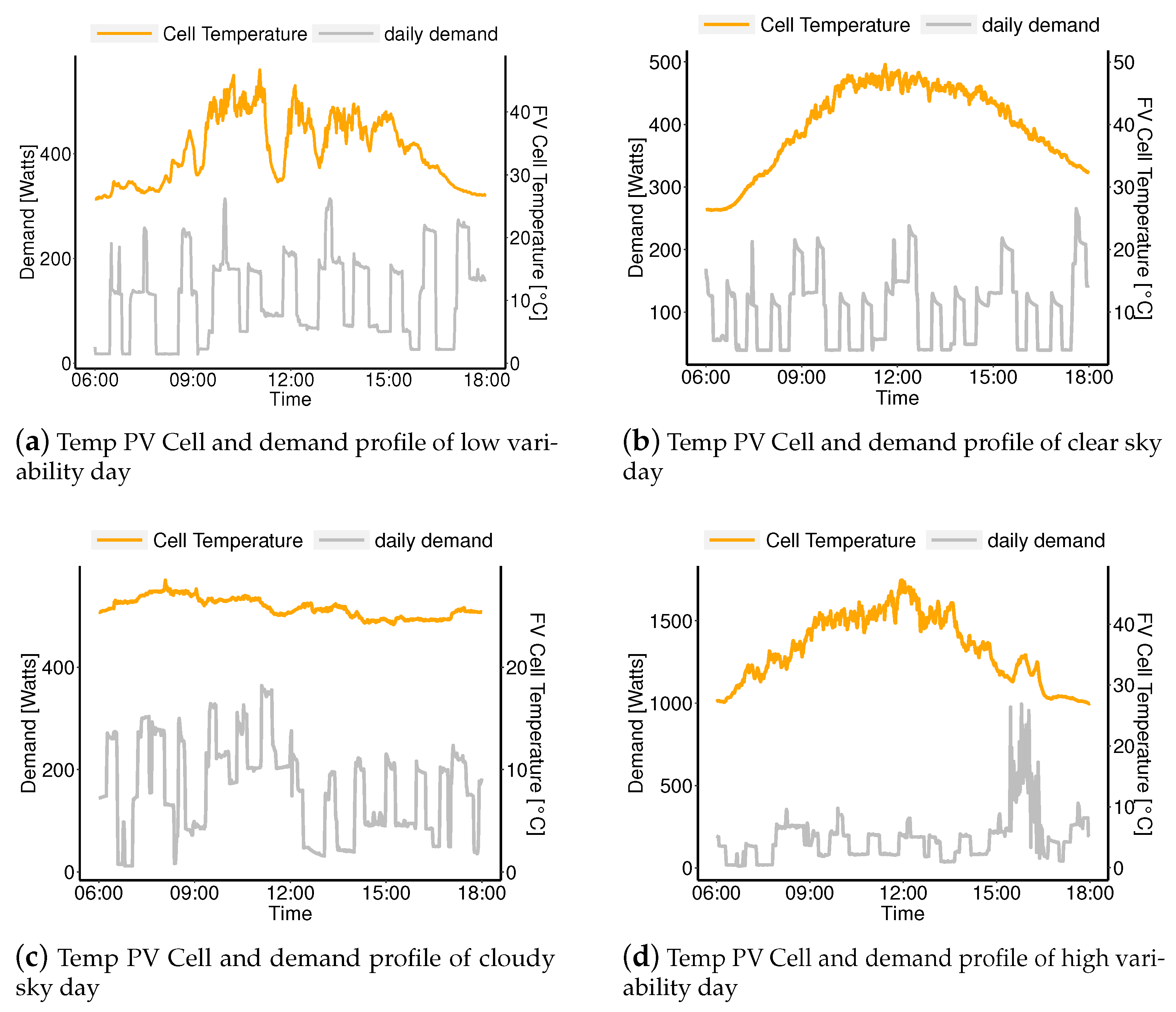
2. Characteristic Profiles of Solar Radiation

The energy incident on the terrestrial surface suffers variations throughout the day, month, year and latitude. The variation of solar radiation is presented in two primordial components: one deterministic and the other stochastic [14]. With a given set of equations inferred from the geographical and geometrical analysis of the position and relative earth-sun movement, it is possible to calculate all the solar resource incident on a generic surface, this fact characterizes the deterministic component [15]. The stochasticity of the solar radiation is given in the alterations of a set of atmospheric factors. One example of this is the randomness of the passing and approaching of clouds and the sporadic shading by passing objects. In short, the behavior of the solar radiation depends on a very complex scenario before the stochastic and deterministic nature. The graphs in Figure 1 contemplate the typical profiles observed on terrestrial surface.

The variability phenomenon is attributed to the weather characteristics of the day in question, evidencing outlines of randomness impacting the daily profile of solar radiation [14]. Such an aspect is quite relevant before the distributed generation scenario, raising the level of risk offered to the electrical system, and the degree of this risk is significantly attached when there is high massive insertion in low capacity networks, for example, remote cities located in islands and away from large urban centers. In this scenario, challenges emerge for the creation of strategies that attenuate the adverse effects caused in the electricity quality [16]. Another overriding factor concerns the location of generators in secondary distribution networks, classified as: residential, commercial, or rural [17]. The secondary distribution networks very often operate asymmetrically, compromising the loads balance, this happens because of varied topologies for connection to the power grid, presented in single phase, two phase, and three phase [18]. That way, it is correct to say, for this context, where an electricity distribution system is equipped with photovoltaic generators, the electricity quality is intimately associated to the power fluctuations and to the charging profile of the power grid.

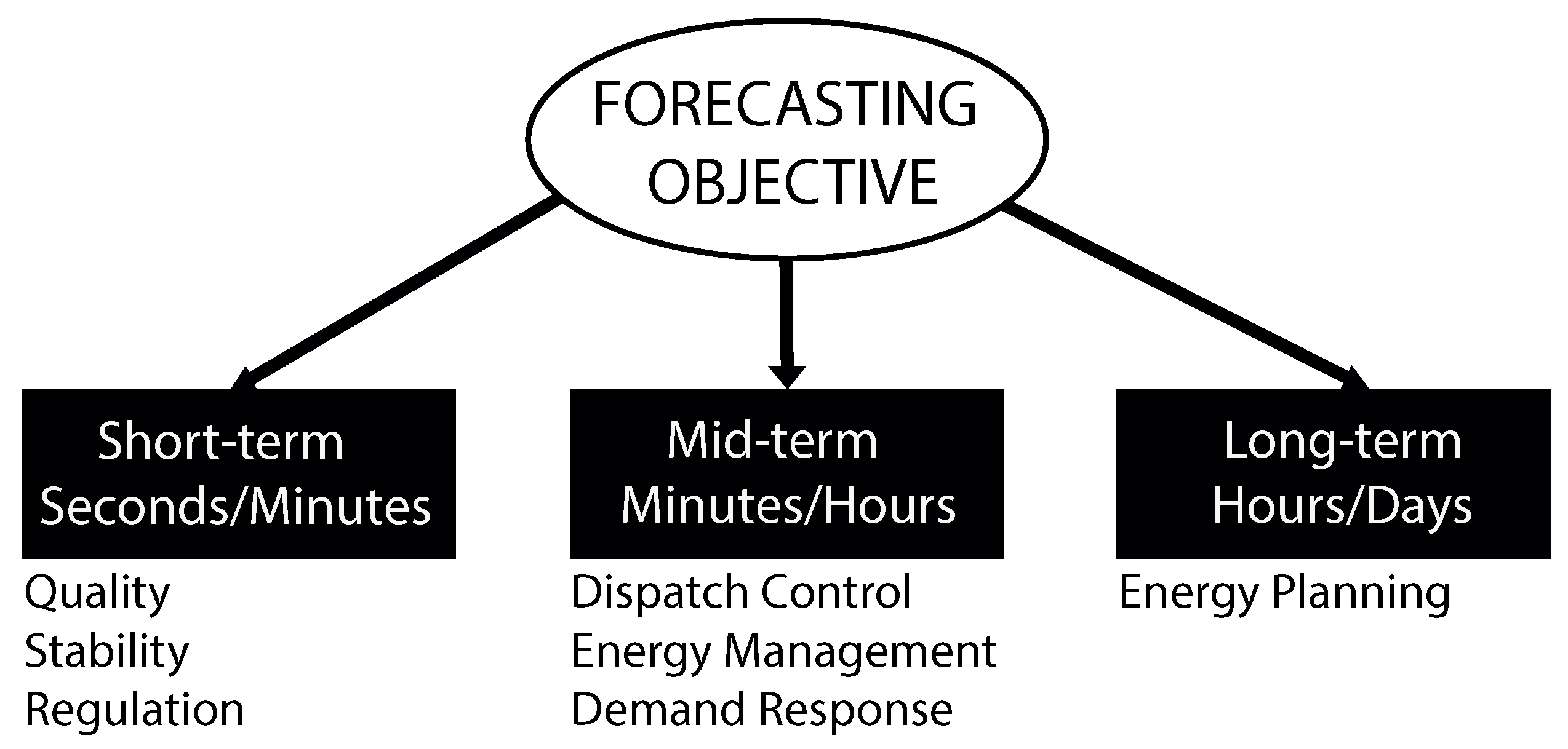
3. Solar Irradiation Forecast

Techniques to forecast the solar radiation have been a much-discussed subject in several research institutes. The well-elaborated forecast helps to plan and operate the electrical system, always implying economic and operational advantages. As regards the problem of guaranteeing the access and the integration of solar energy for all users of the electrical system, it is necessary to adopt measures of mitigation for possible impeding occurrences to the reliable operability of the electrical system mainly before a situation of exposure of a photovoltaic generator to a condition of high variability of the solar resource. Figure 2 associates the objectivity and the utility of the forecasting system as the several procedures and requisitions necessary for the operation of an energy system.

When envisioning an electrical system of conventional power, the quality and stability problems are largely most strongly related to disturbances caused due to too many drives of electrical loads [6]. Going deeper in the definition, the concept of voltage stability then emerges, referring to the ability of a system to recompose and keep the voltage level in permanent regime in all the nodes after being submitted to a stress [19]. However, imagining a scenario of distributed generation in secondary distribution networks, is it foreseeable, the increasing probability of occurrences of momentary disturbances in the electrical system, given the strong correlation between the photogenerated power and solar radiation? In the face of all the reported experiences, new more elaborate techniques emerge daily in order to improve and guarantee the safe insertion of photovoltaic generation. The use of solar radiation forecasting models becomes a crucial task to ensure the operative stability of the network, as well as its expansion [20].

When it comes to short and long-term forecasting, there are several developed predictive models proposed, taking into consideration the geographic localization (latitude), climatological variables associated (radiation, temperature, wind speed, pressure, humidity), prediction time (one minute, five minutes, fifteen minutes, hours, days, months), and models from the simplest, based on the moving averages, to more complex models, using machine learning and artificial intelligence, a thematic that will compose the methodology of this work.

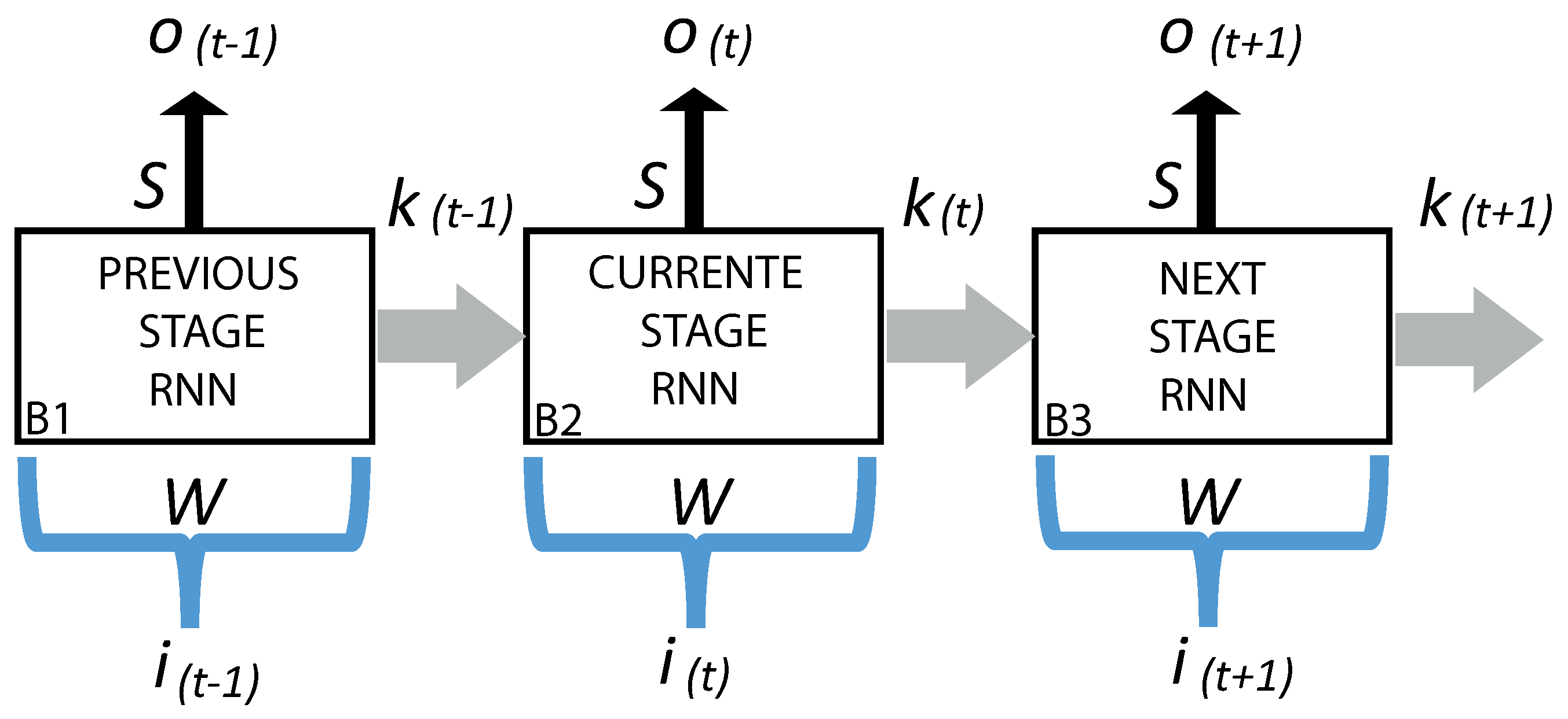
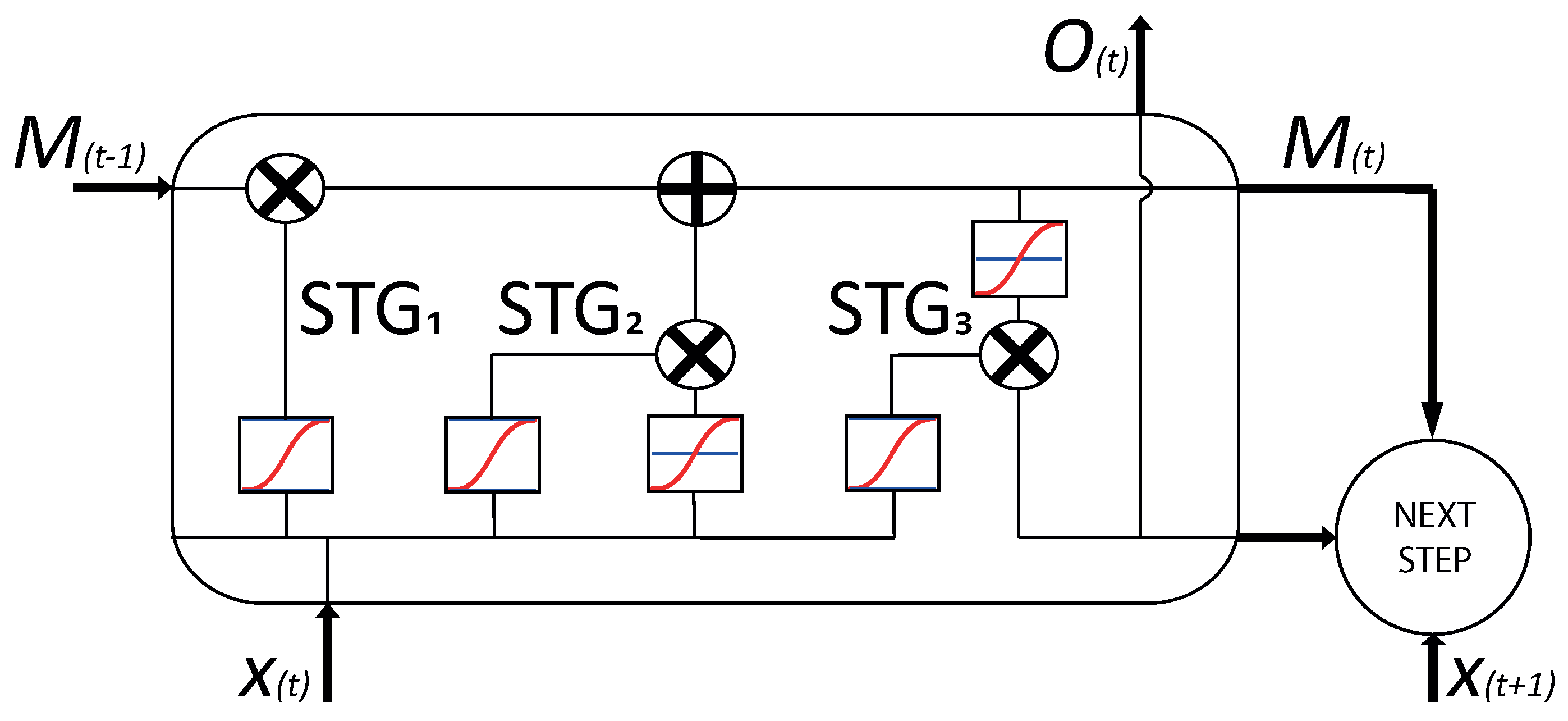
Recurrent Neural Networks

The recurrent neural networks (RNN) have the sensibility of perceiving all the processing history throughout the neural network, the response in function of the input is reached in a complex manner, thanks to the mapping of the entire path referring to the previous inputs, through reverse feeding. For time series with dynamic characteristics, the RNN has high representativeness in terms of efficacy [21]. A simple graphic structuring of this kind of network is presented in Figure 3.

The RNN input parameters are entered at each time step, in Figure 3, and the input sequence is cadenced by the previous time ($i_{(t-1)}$), current time ($i_{\left(t\right)}$), and the predicted time in the future ($i_{(t+1)}$), mathematically symbolized by one vector. Information passed on entry are weighted by a multiplier denoted by W. The output value $O_{\left(t\right)}$ will always take into consideration the information of the previous stage K and the multiplier weigh value S. Considering the stages in Figure 3 where B1 is the processing result in the previous time $O_{(t-1)}$, the current stage (B2) is mathematically expressed by:

$$B2=i_{\left(t\right)}·W+K·B1.$$

(1)

The output of a neural network uses activation functions $\left(\sigma \right)$ and trend constants (c) to delimit the results, considering this parameter, and the output $O_{\left(t\right)}$ in the current stage B2 can be determined by:

$$O_{\left(t\right)}=\sigma ·(S·B2+c).$$

(2)

A derivation of the RNN is the LSTM (Long Short Term Memory). In the work proposed by Wang et al. [21], the advantageous points of LSTM are reported. In Vassalli [22], a detailing is made about the entire operability of the LSTM network. Specific LSTM applications reflected to the production of power from photovoltaic systems were proposed by Abdel-Nasser and Mahmoud’s [23]. In Figure 4, the structural diagram of an LSTM network is presented.

From the representation of an LSTM, Figure 4, the long short-term information is, respectively, denoted by the variables M${}_{(t-1)}$ and H${}_{(t-1)}$. That way, considering a given physical process, the LSTM neural network is able to decide on what is weighted in its learning. Still according to Figure 4, the memory history (M${}_{(t-1)}$) is passed through a filter (forget gate) signed by the multiplication operator located in the upper left portion of Figure 4; in summary, the forget gate (STG${}_1$) controls the information after passing through the sigmoid function. The subsequent stage (STG${}_2$) will include the type of information that will be stored in the cell, and H${}_{(t-1)}$ passes through by a sigmoid filter, again, and a tanh, obtaining the respective numerical values and updating the current state of the cell to M${}_{\left(t\right)}$. Finally, the STG${}_3$ delivers an information preceding the output made compatible by a sigmoid function, generating a real value for the output y${}_{\left(t\right)}$; however, the current state is updated for the short-term memory (H${}_{\left(t\right)}$).

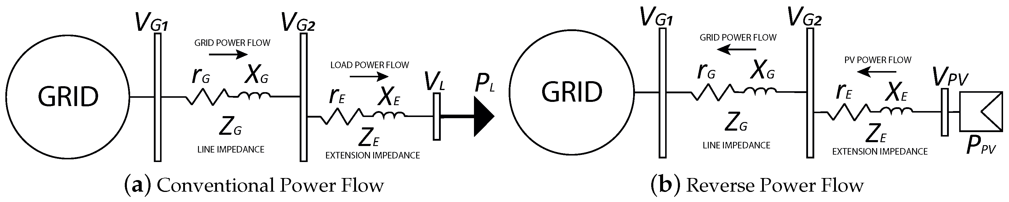
4. Electrical Problems Associated to the High Variability of the Solar Radiation

As mentioned in Reference [24], an electricity consumer can integrate a photovoltaic generator at their residency or business, respecting all technical operative requirements [24,25]. Figure 5 synthesizes separately the power flow dynamics using a simple diagram characteristic of a power system. The representation can be integrated to a more complex system, with more consumer units, nodes, and photovoltaic generators.

When examining Figure 5a, the residential load is directly connected to the network through the Z${}_E$ impedance, and it represents the branch connector responsible for physically interconnecting the residence to the electricity supplier system; this circuit does not share other loads. The equivalent impedance of the network, for simplification purposes, is represented by the variable Z${}_G$, and this element serves to represent the equivalent impedance of the network, seen from the load. The impedances (r + jX) can be presented as function of their resistive (r) and reactive (X) components, and the predominance of both components is dictated by the operative and constructive characteristics of the network influencing the resistance/reactance (X/R) [26]. In addition, in Alves [17], reports regarding the X/R ratio of distribution networks are found, where a strong predominance of the resistive component can take this ratio to a value lower than 1.0. Being $P_L$ the power demanded by the network, the loads in an electric power system represent the global consume, regardless of the consumer class, among the several load models, and the following stand out: power, current, and constant impedance [27], Still referring to Figure 5a, it is emphasized that the low voltage electrical system was initially designed for this operation mode, where the direction of the voltage drop between the nodes is always on the consumer side ($V_G>V_C$). Contrasting this initial analysis, Figure 5b considers the absence of residential load or a relatively tiny one before the photovoltaic generator; then, we have $P_{PV}$ > 0, and, assuming such facts, all the energy flow is reverted to the power grid; in this principle, the voltage in the connection point of the photovoltaic generator will rise in function of the amount of power inserted ($V_{PV}>V_G$).

Both Figure 5a,b represent connections where the load flow will occur in only one direction, sometimes direct, sometimes reverse. Considering initially the energy flow that comes from the source (GRID) to the load ($P_L$), it is possible to formalize the voltage variation mathematically in the source ($V_{G1}$ and $V_{G2}$) and load ($V_L$) sources by the following, Equations (3) and (4):

$$V_{G1}-V_{G2}=I_L·Z_G=I_L·(r_G+j{X}_G),$$

(3)

$$V_{G2}-V_L=I_L·Z_C=I_L·(r_E+j{X}_E).$$

(4)

The network sections of the feeders and secondary distribution branches predominantly present only the resistive components of the impedance due to their electrical and geometric characteristics [18]. In this context, Equation (5) is represented despising the reactive component of the connection branch of the residential consumer unit, expanding it to (6).

$$V_{G2}-V_L=I_L·Z_C=I_L·\left(r_E\right),$$

(5)

$$V_L=V_{G2}-V_{r_E}.$$

(6)

Equation (6) demonstrates that the voltage in the load node is given by the difference between the voltage in the network node and the voltage drop ($V_{r_E}$) throughout the conductor of the connection branch. The branch impedance, for considering, most of the time, the intrinsic factors of the projects, is a simple conductor, and so the impedance is intimately linked to its characteristics, such as: cross section, material used in manufacturing, and linear length of the conductor.

In view of these reflections, the challenge is truly attached in situations of microgenerators positioned in residential preponderance feeders, when it involves the dynamics between the solar irradiance, photogenerated power and power demanded by the residence. A more contemporary view of a low-voltage system is presented by Figure 6.

For the circuit exposed above, the electrical variables $Z_G$, $Z_C$, $V_G$, $V_L$, $P_{PV}$, $Q_{PV}$, $P_L$, $Q_L$, $I_{PV}$, and $I_L$, are, respectively: network impedance, impedance of the consumer interconnection branch, voltage in the network node, voltage at the point of delivery to the consumer, photogenerated active power, photogenerated reactive power, active power demanded, reactive power demanded, photogenerated reactive power, photogenerated current, and current demanded by the consumer unit. For calculation purposes, it is known that the components of active and reactive power compose the respective complex powers.

Maintaining the positive signal convention for the unidirectional current flow and assuming that, in this analysis, $P_{PV}>>P_{LOAD}$, there is the complex power that will flow reversely through the $Z_G$, and $Z_C$ will be obtained by the difference between the complex powers of photovoltaic generation and load:

$$S_{PV,inj}=(P_{PV}+Q_{PV})-(P_L+Q_L).$$

(7)

Assuming that the photogenerated power is higher than the demanded power, the photogenerated current ($I_{inj}$) that will flow from the load node towards the substation node is expressed by:

$$I_{inj}=\frac{P_{inj}-j{Q}_{inj}}{V_L^{*}}.$$

(8)

Polarizing the voltage drop in function of the direction of the current injected by the photovoltaic system, the voltage variation is shown in Equation (9) the potentials are explained through Equation (10), expanded:

$$\Delta V=I_{inj}·Z_E,$$

(9)

$$V_L-V_G=I_{inj}·(r_E+j{X}_E).$$

(10)

With the representation of photogenerated current as a function of power and voltage, the voltage drop in the load node is obtained:

$$V_L-V_G=\frac{P_{inj}-j{Q}_{inj}}{V_L^{*}}·(r_E+j{X}_E),$$

(11)

$$V_L-V_G=\frac{(r_E·P_{inj}+X_E·Q_{inj})+j(X_E·P_{inj}-r_E·Q_{inj})}{V_L^{*}}.$$

(12)

In the work of Borges [18], it is mentioned that the angular aperture between two nodes in a distribution feeder framed in LV grid is practically zero. In Lima et al. [28], the angular invariability between the nodes in the LV distribution system is also reported. Therefore, for the calculation of voltage drop between the nodes, only the real component of the numerator of Equation (12) is considered.

5. Restrictions of Voltage Limits

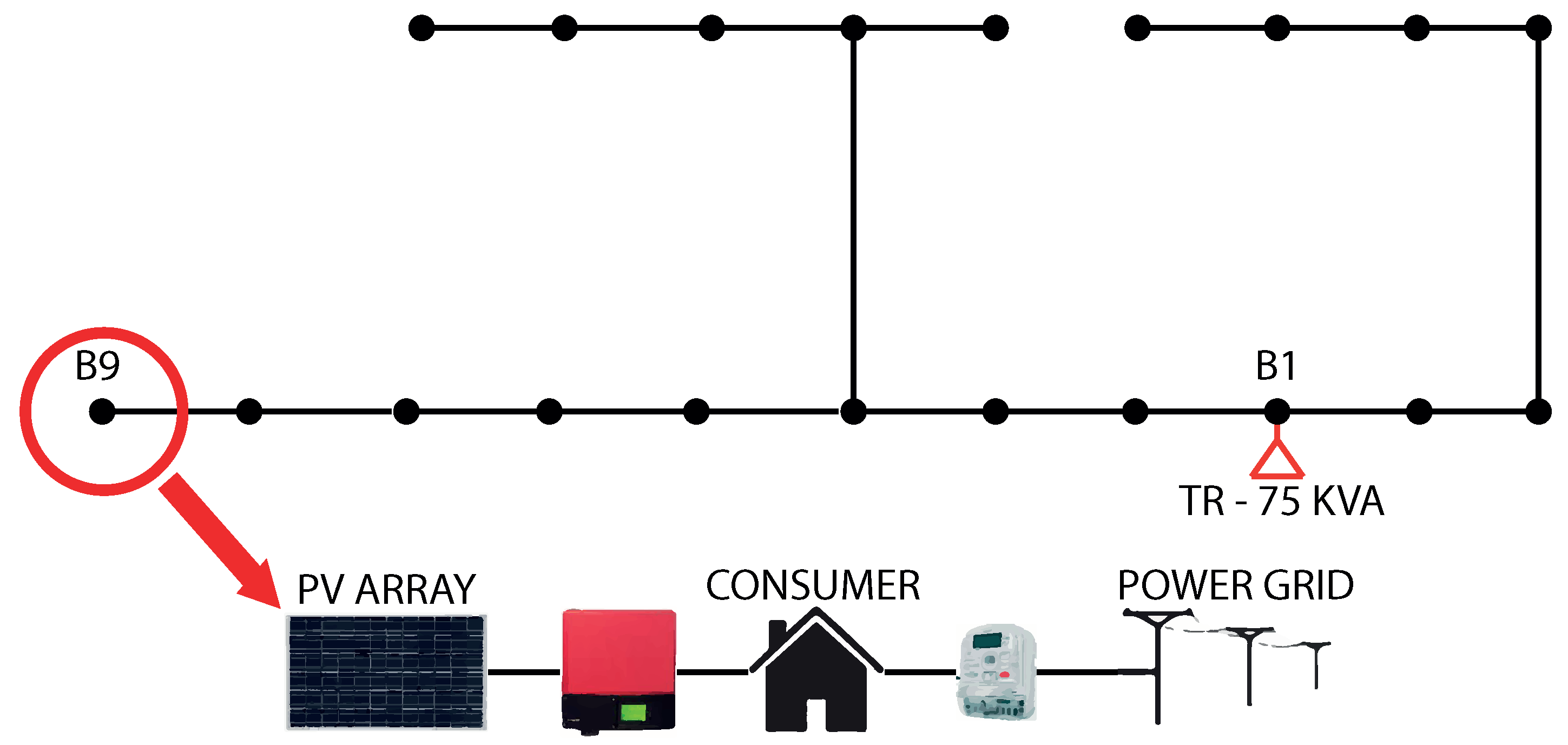
The most common technique for the maintenance of electrical voltage stability is measured by the excitation control of the synchronous generators, the action is performed by the Overexcitation Limiter (OEL) by preventing the injection of reactive power by the synchronous motor [29]. Throughout the transmission and distribution circuits, the voltage stability depends on the transformers, specially to the equipped with the OLTC (On Load Tap Changer) allowing the automatic regulation of the voltage levels throughout the network [30], and this type of equipment is located in medium voltage primary distribution networks serviced in high and medium voltage networks. The graphic representation of the permissible voltage levels is illustrated below in Figure 7.

The steady-state voltage must be monitored throughout the distribution system and the utility must intervene in the power grid in order to ensure the maintenance of the adequate voltage levels. The information in

Table 1. Classification of operational voltage ranges in LV distribution networks.

Voltage Classification	Single Phase 220 V Range (Volts)	Three Phases 380 V Range (Volts)
Normal Operating	$202\le V\le 231$	$350\le V\le 399$
Critical Limit (Upper)	$V>233$	$V>403$
Critical Limit (Low)	$V<191$	$V<331$
Precarious Limit (Upper)	$231<V\le 23$3	$399<V\le 403$
Precarious Limit (Low)	$191\le V<202$	$331\le V<350$

is regulated by the module 8 of the PRODIST, document prepared by the Brazilian agency ANEEL [24]. The table data reflect values only for a given topology, where the base or reference value is in single phase 220 volts or three phase 380 volts. The quality of the voltage level in steady-state voltage level is evaluated by indicators, not exceeding 3% of precarious readings or 0.5% of critical readings within a set of 1008 valid readings [28].

6. Case Study

The current study was motivated by the inconstancies observed in the voltage levels in the attachment point between photovoltaic generator and a residential consumer unit (prosumer), and it is noteworthy that the problem was verified in a real photovoltaic system with operation permission granted by the local utility in the region, properly equipped with climatological sensors instrumentation connected to a referenced CR1000 data logger manufactured by Scientific Campbell. The Logger Net software is responsible for the daily collection of data involved in this study. In this panorama, it was calculated the state of the power grid in the Time-Series mode, at every 1-min interval, considering the presence of photovoltaic generators and the following sky conditions: clear, cloudy, and intermittent. The application was based on a real low-voltage feeder, seen in Figure 8, and more specific parameters and characteristics will be explained next.

Figure 8 presents the real scenario that was modeled in the operational software. The single generator unit present is seen, with rated power of 5.1 kWp and synchronized in the network before the B9 node downstream from the substation (TR-75 KVA) which makes the energy flow available for the circuit, where the primary of the respective transformer is connected in delta $(\Delta )$, and the secondary is connected in star (Y), with three phase voltages of 13.8 kV and 380 V, respectively. The interconnection point was monitored to serve as a basis for simulation studies.

Table 2. Electrical data of the real feeder.

Line	Start	End	Length (m)	Line	Start	End	Length (m)
1	B2	B3	31	11	B12	B13	25
2	B3	B4	34	12	B10	B14	18
3	B4	B5	20	13	B14	B15	17
4	B5	B6	31	14	B2	B20	10
5	B6	B7	32	15	B20	B19	40
6	B7	B8	27	16	B19	B18	32
7	B8	B9	42	17	B18	B17	30
8	B4	B10	40	18	B17	B16	30
9	B10	B11	22	19	B16	B15	20
10	B11	B12	24

presents the layout of the lines and nodes that configured the power grid under study.

The characteristics of the cable that compose the stretches of the circuits are shown in

Table 3. Specifications of the conductors used in the feeder.

Line	Conductor	Line Position	Line	Conductor	Line Position
1	Al70 mm2	Trunk	11	Al25 mm2	Middle
2	Al70 mm2	Trunk	12	Al25 mm2	Middle
3	Al70 mm2	Trunk	13	Al25 mm2	Middle
4	Al50 mm2	Middle	14	Al50 mm2	Neutral
5	Al25 mm2	Trunk	15	Al50 mm2	End
6	Al25 mm2	Trunk	16	Al50 mm2	Middle
7	Al25 mm2	End	17	Al50 mm2	Middle
8	Al25 mm2	End	18	Al70 mm2	Trunk
9	Al50 mm2	Middle	19	Al70 mm2	Trunk
10	Al25 mm2	Trunk

, where it is possible to associate the electrical characteristics of each conductor and their physical location in the stretches of the circuit associated to the column “Line” of Table 2 and Table 3.

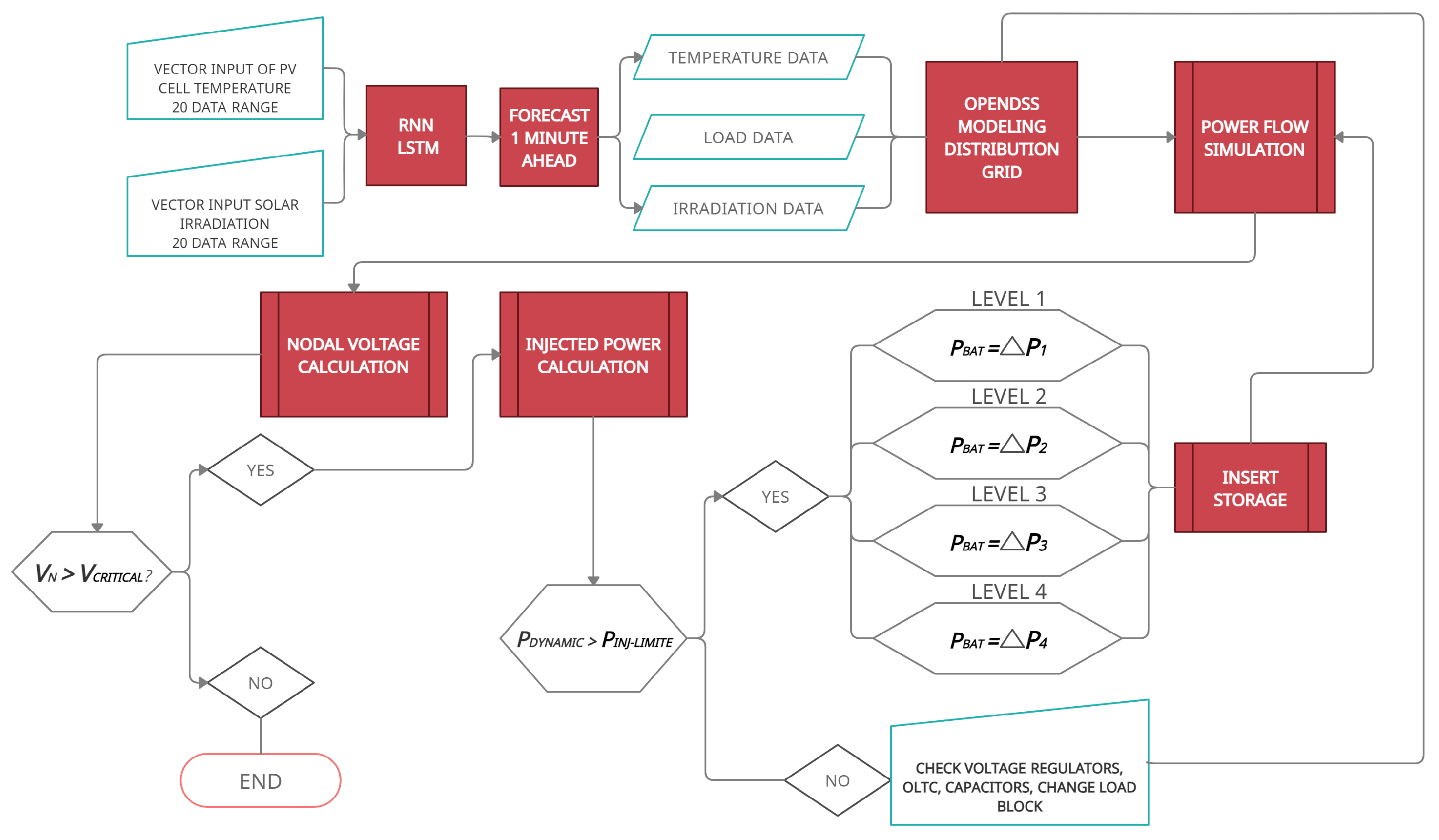
7. Mitigation Method for Overvoltage

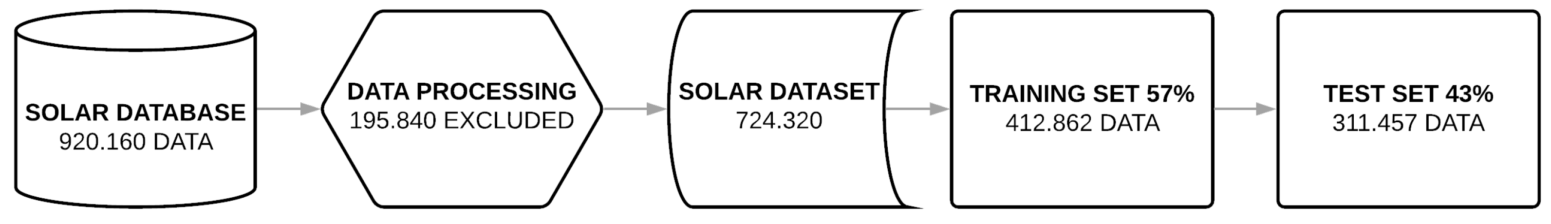
The purpose of this work is to mitigate overvoltages by anticipating the state of the power grid of a low voltage distribution circuit through the irradiance and temperature prediction tool of the photovoltaic cell in the generator arrangement. Thus, the calculation of the power flow is performed providing the results 1 min in advance, guaranteeing the precise decision making of the storage system. An illustration of the proposed method is shown in a flowchart format in Figure 9 below.

The ultimate goal of this method is to ensure voltage regulation below the critical value. The goal of the initial stage, addressed by the power flow forecasting and calculation stages, is fundamental to feeding the model comparison block, based on the comparative results, and the need to insert the storage is decided and estimating the convenient level of battery power ($P_{BAT}$). The first verification step compares the rated voltage ($V_N$) with the critical voltage, according to the normative resolution of the module 8 do PRODIST [24], informed in Section 5. The comparison block, that limits the power injection ($P_{inj-limit}$), started from a permission threshold of $P_{inj-limit}=2500$ W; this value was used by analyzing the time series for 1 year of operation of the photovoltaic system used in Reference [4], observing the data of power injected into the distribution network and the voltage level at the common coupling point; with this, for this condition, the value of $P_{inj-limit}=2500$ W, it was correlated with 5% of the occurrences of overvoltage. It is noteworthy that there is no rule for establishing the power injection limit in the electric network, and the limitation is only considered in function of the available capacity of installed power in a given point of the electric network, supported by the norm of the local operator of the power system. distribution.

7.1. Database

The database used in this work was composed by a historical series of incident irradiance in the location of the study over a 21-month time horizon (1 January 2019 to 30 September 2020), the equivalent of 639 days. In addition to global irradiance, the operational temperature of the modules that equip the photovoltaic generator were registered, and the electrical magnitudes (voltage and direct current, power in alternating current, and network electrical voltage) were also collected. It is worth mentioning that the time interval of acquisition and registration of variables was of one minute; that way, 1440 data per day was obtained for each variable. The making of the database in this work was previously preprocessed and filtered to ensure the integrity of future results and the performance of the model of the neural network. After the refinement of the data, 503 days were defined, totaling approximately 725 thousand records of all the variables in the process. Data were segregated for the training actions and RNN LSTM test, arranging in 412 thousand and 311 thousand records, respectively. The procedure described can be seen in Figure 10.

The modeling of the distribution network and its elements was the same considered in Section 6. For greater real representativeness in the results, some demand meters were used in the CUs adjacent to the resistance where the photovoltaic generator is located in order to record possible impacts in the voltage through the operational dynamic of the loads. The measure data in the adjacent CUs will serve also as parameters for future simulations in order to obtain better results in the simulations of the state of the network and the calculation of the voltage. To illustrate, after Figure 11, the composition of the demand curves and the operational temperature of the photovoltaic module regarding specific days are presented and will be used in the simulation of a CU equipped with the photovoltaic generator. Each subgraph below is associated with a condition typical of solar irradiation. Thus, the days of low variability, clear sky, cloudy sky, and high variability, refer, respectively, to days, 1, 2, 3, and 4.

The dataset presented in the graphs above are relevant as input parameters in the simulation with OpenDSS to perform the power calculation in the Time-Series mode. It should be noted that the inverter efficiency curve and the rated characteristics of the photovoltaic generator are necessary for this calculation.

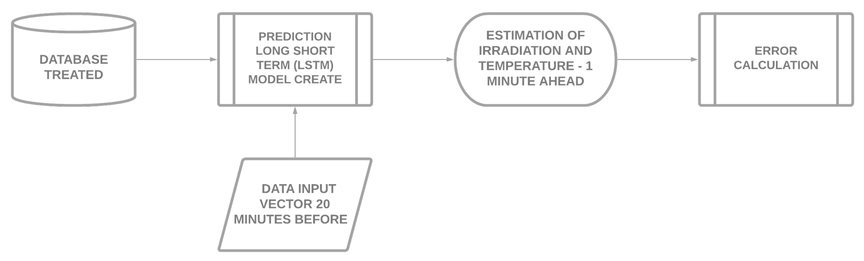
7.2. Forecasting Model of RNN LSTM

The combination of the solar irradiation forecast and the solution of the power flow from the feeder modeling results in the ability to anticipate the variability of the electrical voltage of the network caused by the high variability of the solar irradiance. The motivation to develop this method is intimately connected to the peculiar characteristics of the low-voltage network, such as: infrastructure, absence of instantaneous and retroactive information of the electrical variables, low level of electrical protection, and strong alterability of electrical loads. It should be noted that, for an installed capacity in a feeder, if there is a greater number of photovoltaic systems installed with lower power than the number of photovoltaic systems with higher power, there may be a situation of limitation of the hosting capacity much earlier in the first case than in the second. In this aspect, we come to the big questions: What is the maximum hosting capacity of the distributed generators in the feeder in question? The engineering professionals are able and equipped to analyze and grant permission for the insertion of distributed generators to the network, admitting reliability and operational security to it? The crucial point of the purpose of this study is attributed to the performance of the LSTM network, and this is where the solar irradiance forecast information will be sent. The first part of the proposed model is formed by the forecast stage set in a recurrent neural network LSTM type. The model was built and tested as explained in the previous topic, illustrated by Figure 10. Below, Figure 12 shows the flowchart of the steps of the definition and validation of the model of the neural network used.

The model defined runs the solar irradiance forecast for every 1 min ahead, based on the 20-min retroactive information from historical series of solar irradiance measured by the local solarimetric station. In parallel, the photovoltaic sensor serves as a reference standard for the predicted value, and for future recalibrations of the LSTM neural network. The concern with having a high performance for the neural network is vital for the subsequent steps, of the global method (Figure 9), to reach an accurate and coherent value.

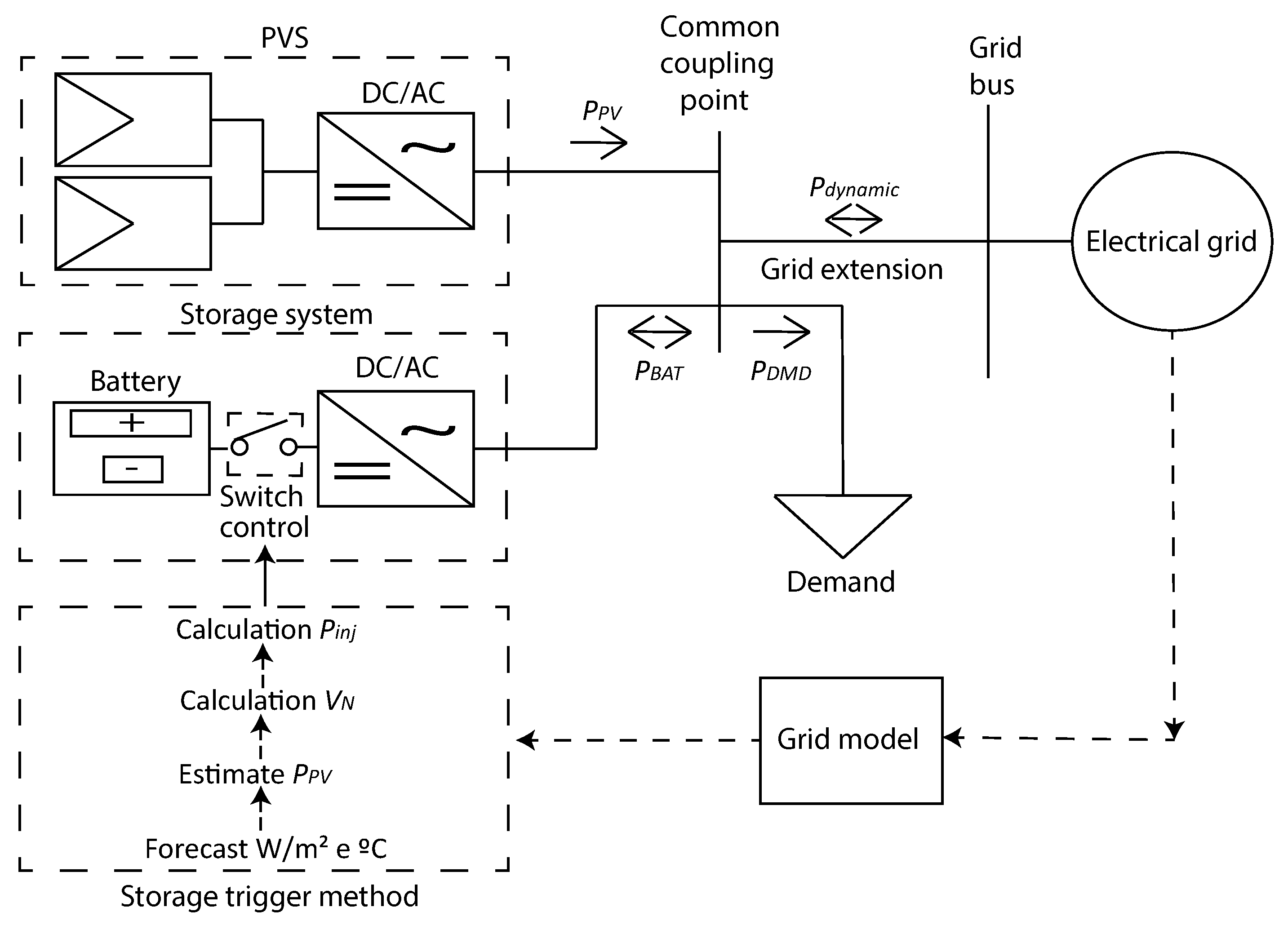
7.3. Storage System Planning and Definition

The battery system can be allocated directly in direct current (DC) next to the photovoltaic modules or it can be connected directly to the power grid through an interface converter to synchronize and make the batteries compatible with the electrical system. In this work, the control of the battery is centered primarily on the forecast of solar radiation and the temperature of the photovoltaic cell; after that, considering a feeder already modeled, the power flow is calculated through OpenDSS, allowing verification of both voltages nodal as the powers injected into a bar. These results allow us to infer about the voltage levels, framing them in the operational restrictions. In practical terms, a view of the elements that make up the network with their respective variables is shown below in Figure 13.

The planning of the instantaneous drive was initially based on the dynamic power situation ($P_{dynamic\left(t\right)}$) that flows through a connection branch in a UC. The dynamic power is due to the conditions of generation and demand, and a mathematical understanding is shown below, interpreting when any UC is operating under the condition of direct flow (consuming electrical energy), reverse (providing electrical energy), or in equilibrium (autonomous), as shown in (13). The dynamic power is calculated by the difference between the power generated ($P_{PV}$) and that consumed ($P_{DMD}$) by the residence, being defined the operation profile of the storage system:

$$P_{dynamic\left(t\right)}=P_{PV\left(t\right)}-P_{DMD\left(t\right)}=\left\{\begin{array}{cc}\hfill DirectFlow,& \mathrm{If} (P_{PV}<P_{DMD})\hfill \\ \hfill ReverseFlow,& \mathrm{If} (P_{PV}>P_{DMD})\hfill \\ \hfill Autonomous,& \mathrm{If} (P_{PV}=P_{DMD})\hfill \end{array}.\right.$$

(13)

Under the condition of reverse flow, the idea of using the storage system is to limit the dynamic power, which flows through the grid extension that connects the common coupling point with the grid bus, to a maximum limit power, previously defined ($P_{inj-limit}$). Every moment that $P_{dynami{c}_{\left(t\right)}}$ > $P_{inj-limi{t}_{\left(t\right)}}$, there is a need to actuate the storage system through the control key, framing the storage system in passive mode. With this, the passive power of the battery bank ($P_{BAT}$) is calculated in:

$$P_{BA{T}_{\left(t\right)}}=P_{dynami{c}_{\left(t\right)}}-P_{inj-limi{t}_{\left(t\right)}}.$$

(14)

The modes of operation of the storage system are translated by the conditional Equation (15), from the result of the difference between photovoltaic generation and demand. The signal adopted for $P_{BAT}$ uses the positive convention for loading and negative for unloading. The conditions regarding the operation of the battery in terms of its operating mode (Charge, Discharge, and Idle) is interpreted by the following conditions:

$$P_{BAT}=\left\{\begin{array}{ccc}\hfill Charge,& \mathrm{If} (P_{{PV}_{\left(t\right)}}>P_{{DMD}_{\left(t\right)}}) \hfill & \mathrm{and} (P_{{dynamic}_{\left(t\right)}}>P_{inj-limit})\hfill \\ \hfill Idle,& \mathrm{If} (P_{{PV}_{\left(t\right)}}>P_{{DMD}_{\left(t\right)}}) \hfill & \mathrm{and} (P_{{dynamic}_{\left(t\right)}}<P_{inj-limit})\hfill \\ Idle,\hfill & \mathrm{If} (P_{{DMD}_{\left(t\right)}}>P_{{FV}_{\left(t\right)}})\hfill & \hfill \\ \hfill Discharge,& \mathrm{If} (P_{{FV}_{\left(t\right)}}=0)\hfill & \mathrm{and} (\forall P_{{DMD}_{\left(t\right)}})\hfill \end{array}.\right.$$

(15)

The value of $P_{BAT}$ is closely linked to the value of $P_{inj-limite}$, since, if the power limitation value is too low and the bank’s capacity remains the same, it will reflect in the increase of depth of discharge of battery’s (DoD), consequently reducing its useful life. As there is no rule for dimensioning the coefficient of $P_{inj-limit}$, it is important to pay extra attention when assigning its value, as two situations can occur: high cost of implanting the batteries or inability to mitigate overvoltages due to early charging. For such a context, it is necessary to increase the capacity of the battery bank in order to maintain the state of charge (SoC) within an operational range that optimizes the life of the batteries. In Diaz [31], a method for calculating the battery capacity is presented can be calculated by the difference between the minimum and maximum limits. The capacity of the storage system can also be obtained by integrating $P_{BAT}$, present in Equation (14).

The signal convention for the storage system operating modes is linked to a component $P_{BAT}$.

Table 4. Summary table of the drive profile of the storage system.

Operation Mode	Battery Power	PV Power	Demand Power
Charge (Passive)	$P_{BAT}$ > 0	$P_{PV}$ > 0	$P_{DMD}$ > 0
Idle (Neutral)	$P_{BAT}$ = 0	$P_{PV}$ > 0	$P_{DMD}$ > 0
Discharger (Active)	$P_{BAT}$ < 0	$P_{PV}$ = 0	∀$P_{DMD}$

, below, synthesizes the mode of operation according to the main variables involved in the process.

The storage system was made possible at 4 power levels. The purpose of this configuration seeks to provide greater flexibility in the insertion of power; in addition to that, in the event of eventual maintenance of the device, this context would guarantee partial operation. Each power level corresponds to a $\Delta P$ different, where the first step is to limit the dynamic power that will be injected into the network to the minimum limiting values ($MIN\left(P_{inj}\right)$) and maximum ($MAX\left(P_{inj}\right)$). In that regard, the minimum value of the injected power is equal to the limit value of the power injection defined at the beginning of this section; thus, $MIN\left(P_{inj}\right)$ = $P_{inj-limit}$, and the maximum values will be arbitrated for every 500 W step increase. $\Delta P$ as a function of the dynamic power for each level is obtained from the set of inequalities below:

$$\Delta P\left(P_{dynamic}\right)=\left\{\begin{array}{c}500W,\mathrm{If} MIN\left(P_{inj}\right)\le P_{dynamic}\le MAX\left(P_{inj}\right),\mathrm{for} MAX\left(P_{inj}\right)=3000\mathrm{W}\hfill \\ 1000W,\mathrm{If} MIN\left(P_{inj}\right)\le P_{dynamic}\le MAX\left(P_{inj}\right),\mathrm{for} MAX\left(P_{inj}\right)=3500\mathrm{W}\hfill \\ 1500W,\mathrm{If} MIN\left(P_{inj}\right)\le P_{dynamic}\le MAX\left(P_{inj}\right),\mathrm{for} MAX\left(P_{inj}\right)=4000\mathrm{W}\hfill \\ 2000W,\mathrm{If} MIN\left(P_{inj}\right)\le P_{dynamic}\le MAX\left(P_{inj}\right),\mathrm{for} MAX\left(P_{inj}\right)=4500\mathrm{W}\hfill \end{array}.\right.$$

(16)

The total electrical energy given off in charge mode by all levels of the storage system is calculated from the sum of the individual energy of each $\Delta P_{BAT}$. The following, Equation (17), calculates and converts the global energy stored by the battery bank in Watt hour (Wh).

$$C_{BA{T}_{\left(t\right)}}=\frac{1}{60}\left[\sum _{t=1}^n{P}_{BA{T}_{Level1}}\left(n\right)+\sum _{t=1}^n{P}_{BA{T}_{Level2}}\left(n\right)+\sum _{t=1}^n{P}_{BA{T}_{Level3}}\left(n\right)+\sum _{t=1}^n{P}_{BA{T}_{Level4}}\left(n\right)\right].$$

(17)

The charging for the mitigation of the storage system will start from a minimum state of charge of 70% of the total capacity of each level of the storage system, in such a way that, when the batteries need to discharge, usually at night, only 30% of the stored energy will be discharged. It is also noteworthy that the discharge depth will be variable; that is, in the condition of full charge, the maximum discharge depth will be 30%, and for an operating situation where it was not possible to fully charge the battery, the depth discharge will be relatively lower. This work is limited only to highlight the passive study of storage, so, in this stage, the battery discharge mode will not be considered.

8. Results

In this section, the results will be separated by topics, and each step will be discussed in isolation. In the end, the performance of the proposed method to mitigate the overvoltage promoted by the power produced by photovoltaic generators will be performed from a comparison with the voltage obtained experimentally if the system was operated on the respective days.

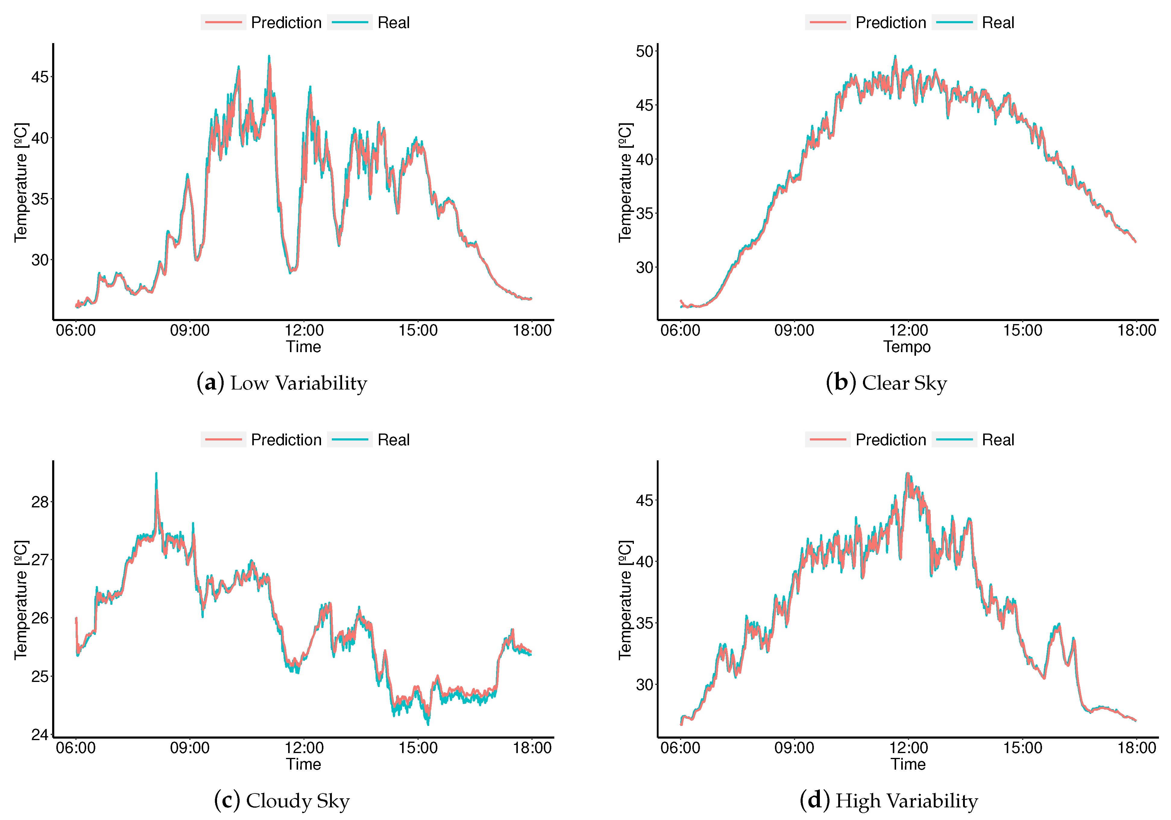
8.1. Result of the Forecast of Solar Irradiation and Cell Temperature

The estimation of the solar radiation and temperature of the photovoltaic module cell is the first task of the method,; all results practically derive from this function. As the objective is to ascertain the impact of the variability of the solar resource, as well as the mitigation in these conditions, and the results of this stage show only the days with the following climatological peculiarities: clear sky, cloudy sky, low variability, and high variability, in order to evaluate what each particularity of these days influence in the power grid.

For the prediction of solar radiation, the last 20 values were used, and the next value was estimated based on the trained model of the LSTM; therefore, the errors were calculated to evaluate the accuracy of the model. The RMSE calculated for the output values of the LSTM neural network reached a value of 78.52 W/m², along with a linear correlation coefficient of 96%. Right after, the graphs for the 4 typical days explained in Figure 14 are presented.

The visual perception of the predicted and real solar irradiation graphs shows a great similarity in their behaviors, which are statistically ratified by the regression coefficient R² close to 95%, and

Table 5. Performance of solar irradiation forecast.

Day	Day Classification	RMSE (W/m2)	MAE (W/m2)	R2
Day 1	Low variability	96.39	58.03	0.93
Day 2	Clear sky	47.84	33.44	0.99
Day 3	Cloudy sky	5.69	3.56	0.97
Day 4	High variability	121.36	73.47	0.89

individualizes the performance results for each day. The performance parameters were compared with solar irradiation data measured by the datalogger, covered in Section 7.1; more details about the instrumentation and the measurement can also be seen in Section 6. Table 5 shows the performance information around the statistical metrics, RMSE, MAE, and Pearson, thus determining the accuracy of the prediction algorithm.

The biggest error found was for the classification of the sky of high variability. The lowest values of RMSE were related when the forecasting model ran a day with lower rates of variability, that is, on days of clear or heavily cloudy skies, Figure 14b,c. On those days, the correlations between the simulated and the experimental profiles resulted in 0.99 and 0.97, respectively. In contrast, on the days of intermittent behavior with low or high variability, Figure 14a,d, the mean quadratic error increased to 96.39 W/m² and 121.36 W/m², respectively, followed by their respective Pearson coefficients of 0.92 and 0.89.

In the work of Campos Filho [14], an RMSE of 179.4 W/m² was found for a set of 267 1-min predicted data samples, and the forecasting system used was based on image processing. In the article published by Alzahrani et al. [32], a normalized RMSE of 0.078 for an LSTM neural network was verified; it is noteworthy that the author used a database of 4 days of measurement of solar irradiation acquired from a LI-200S sensor, in a sampling frequency of 100 Hz. In the article by Guariso et al. [33], a performance test of some prediction models was carried out; the author slices the results in a short term horizon (5 min) for the first three hours of the day, and the RMSE obtained by RNN LSTM, only with daily data, was 121.78 W/m². The interesting fact is that this result is very close to the value found for the day of high variability in this work, and the database that the author uses in his work is composed of 60% of the data classified as cloudy and partially cloudy.

Concomitantly, the prediction of solar irradiation in parallel with the prediction of the operating temperature of the cell was carried out, and the two information sets serve as subsidies for the calculation of the photogenerated power. In practical terms, the neural network provides a set of information on solar radiation and the cell’s operating temperature for the respective days of interest. Soon after, in Figure 15, follows a graphical perspective of the results obtained by the predictor system compared to those measured experimentally.

The comparison between predicted and experimental data is compared based on performance metrics. The RMSE between the predicted and experimental value for the day of low and high variability, reached a value of 0.80 ${}^{\circ }$C and 0.69 ${}^{\circ }$C, respectively. For the clear day, the RMSE was close to 0.41 ${}^{\circ }$C; for the cloudy day, the calculated RMSE was 0.13 ${}^{\circ }$C. Some reports in the literature seek to evaluate the performance of the model according to the size of the observed data window. Chevalier et al. [34] obtained a better performance of the network using 24 data from past observations. In his thesis work, Sabino [35] found an RMSE between 0.6 ${}^{\circ }$C to 1.6 ${}^{\circ }$C varying in a time horizon of 1 h up to 24 h. The error values found in this work are in line with those found in the literature, thus enabling the application of these results in the next stages of this research.

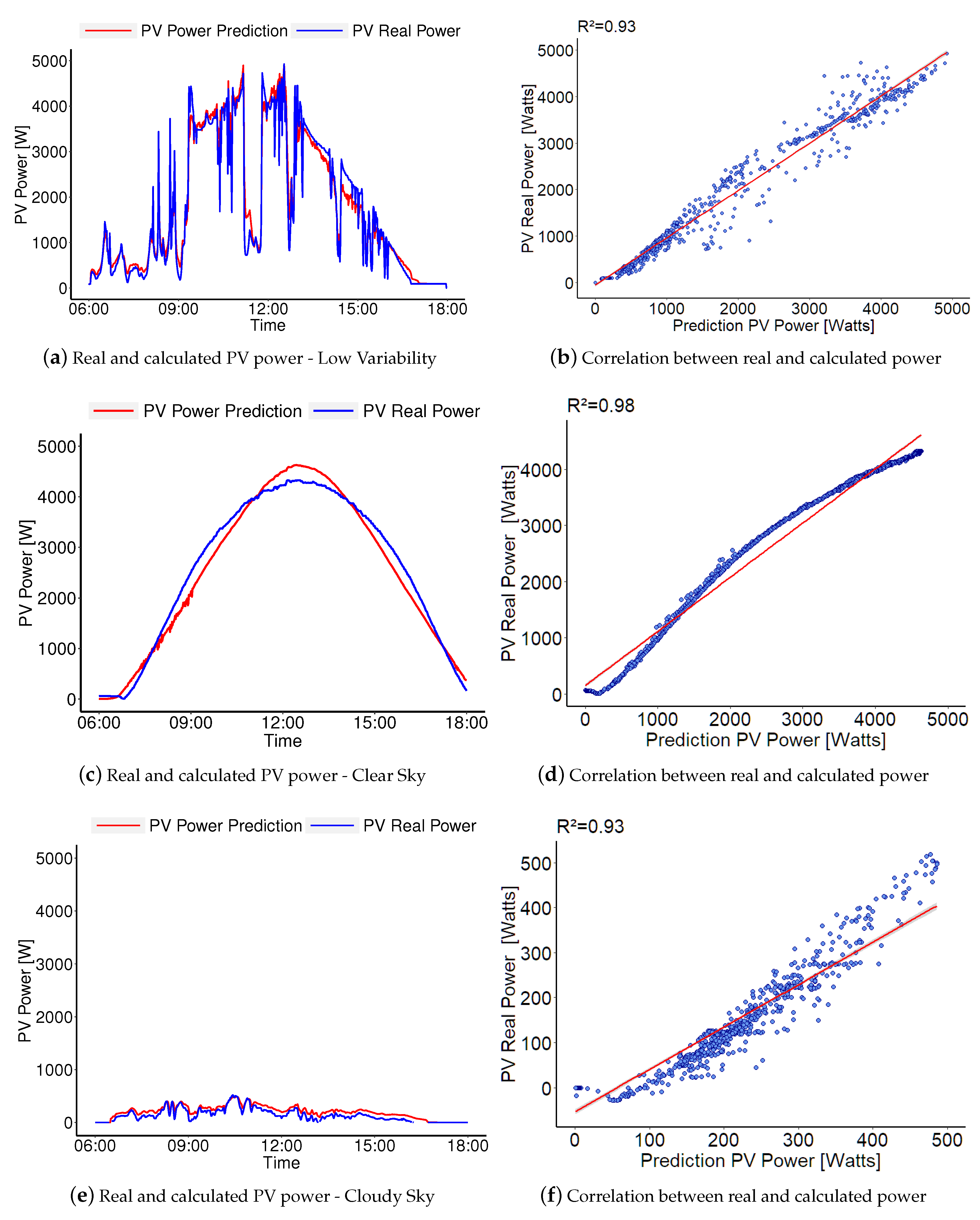
8.2. Determination of Power Flow Produced by the Photovoltaic Generator

In this step of the study, the photovoltaic generator power values of 5 kWp were obtained, considering the real solar irradiation and the previously simulated, in addition to the modeling of the distribution feeder, and, parameterizing and replicating all its real characteristics in the simulation computational environment in the OpenDSS, were elaborated from the answers of simulations of the LSTM neural network, observed in Figure 14. Next, the graphs in Figure 16 show a comparison between the real data monitored by an active power transducer in the alternating current (AC) output of the inverter and the power. Both the simulated values (Nowcasted) and the measured values were sampled every 1 min.

The power flow presented in graphical form in Figure 16; sketches on the left instant comparative of experimental electrical power and Nowcasted, and on the right are the representation of linearity between them, for various sky conditions profiles, along with the representation of linear dependency between predict and real magnitudes. Similar to what happened to solar irradiation in the previous section, when comparing the real power curve and calculated curve, a RMSE of 77.29 W was observed in a cloudy sky day, while, on a clear sky day, a RMSE of 230.91 W was reached. In reference to Pearson’s correlation, coefficients on a clear sky day resulted in 0.98 and 0.93 in cloudy sky days. This occurs because, on cloudy sky days, the photovoltaic system operates in lower load for most of the day, resulting in imprecise measurements because the transducer operates out of its optimum point.

For days characterized as intermittent, the error metrics were established close to each other. The higher RMSE value for the power was slightly higher for the day with low variability Figure 16a, reaching a root-mean-square error of de 276.21 W, in terms of percentage variation; the day with low variability was 0.76% above the RMSE obtained for the day with high variability, in Figure 16d, in which a RMSE of 274.12 W was calculated. In general, the calculation for PV power production shows good fidelity, considering an average of all variables between the days analyzed, and there are good linear correlation metrics (R² = 0.96), root-mean-square error (RMSE = 214.57 W), and mean absolute error (MAE = 173.60 W) for the data estimated and observed in a period of 12 h (6:00 a.m. to 6:00 p.m.).

The low loading of consumer units during too many solar irradiation rates favors the emergence of overvoltages. It is noteworthy that the power flow simulation for the state of the network was calculated using the time series of the demand curve for the respective days. In Figure 17, the combination of factors that corroborate the intensification of the power injected into the network are presented, delivered in the form of reverse power flow, another factor that justifies the voltage overshoots. With the confirmation of the rated voltage above the critical voltage, the proposed method performs the next step, performing the calculation of the injected power and conditioning it to the allowed limit ($P_{inj-limit}$ = 2500 W) previously predifined. For each day, the following figure shows the reverse flow ($P_{dynami{c}_{\left(t\right)}}$) detecting the moments when the permission for injection limit value is exceeded.

In practical terms, the cloudy day is the only one that observes the lowest injected reverse power, justified by the low index of solar irradiation; in addition to this fact, the demand profile also helps in the reduction of the reverse power. This analysis already confirms that the injected power limit is not exceeded, ending the process. On the other hand, on the days with the highest activity of solar irradiation, for high variability, 30% of the occurrences of exceeding the power limit were obtained when compared to the day of low variability. The day of clear sky surpasses the day of high variability in instances of exceeding the power limit, reaching 33% more occurrence than the day of high variability. In

Table 6. Summary of simultaneous occurrences.

Classification	${\mathit{V}}_{\mathit{N}}$ > ${\mathit{V}}_{\mathit{critical}}$ ${\mathit{P}}_{\mathit{dynamic}}$ > ${\mathit{P}}_{\mathit{inj}-\mathit{limit}}$	${\mathit{V}}_{\mathit{N}}$ < ${\mathit{V}}_{\mathit{critical}}$ ${\mathit{P}}_{\mathit{dynamic}}$ > ${\mathit{P}}_{\mathit{inj}-\mathit{limit}}$	${\mathit{V}}_{\mathit{N}}$ > ${\mathit{V}}_{\mathit{critical}}$ ${\mathit{P}}_{\mathit{dynamic}}$ < ${\mathit{P}}_{\mathit{inj}-\mathit{limit}}$	${\mathit{V}}_{\mathit{N}}$ < ${\mathit{V}}_{\mathit{critical}}$ ${\mathit{P}}_{\mathit{dynamic}}$ < ${\mathit{P}}_{\mathit{inj}-\mathit{limit}}$
Low Variability	15%	18%	0%	67%
High Variability	31%	11%	0%	58%
Cloudy Sky	0%	0%	0%	100%
Clear Sky	11%	46%	0%	43%

, below, are the metrics of overvoltage and over power as a function of the total time period analyzed.

The data explained in Table 6 reveal the frequencies of occurrences of the total time that exceeded both the critical voltage and the limit power, simultaneously. It is noticed that the greatest impact on the tension occurs on the day of high variability, marked at 33%, while the overpower is registered at 43%; this information is significantly above the numbers obtained for the day of low variability. The curious fact is revealed for the day of clear sky, where there is the highest percentage of occurrences of the power overrun. In contrast, the overruns of the voltage limit is minimally represented by 12% of the events that occurred. This condition is associated with the absence of power fluctuations for a clear day, allowing the power to be injected into the distribution system smoothly, without providing severe disturbances in the power grid.

8.3. Short-Term Voltage Regulation

The final step presents the results of the calculated stress profile compared to the mitigating stress profile, obtained through the proposed method based on the storage system. The attributes inserted in Table 6 are used to measure the phenomenon of overvoltage in simultaneous events, in addition to illustrating the global panorama of the events that occurred in the simulation. The solution of the problem was carried out in a period of 12 h, totaling a dataset of 720 samples for the classifications of the type of sky used in this work.

In Figure 18, all the graphics on the left side depict the dynamic effect of inserting the storage system in mitigating short-term overvoltage. The green curve, called the nominal voltage, is under the absence of the mitigation strategy. The blue curve alludes to the voltage profile submitted to the mitigation strategy. The composition of the images in Figure 18 was prepared in pairs, concatenating the voltage graph with the respective power graph drained by the storage system.

The strong relationship between the voltage at the supply point and the reverse power flow is quite evident in all scenarios. Taking the high variability day as an example, the storage system drains approximately 5042 Wh of electrical energy; this amount corresponds to 22.56% of the useful energy that would be injected into the distribution network by the photovoltaic system. The clear sky day, highlighted by having a large volume of electricity production, manages to minimize the storage of electricity in the battery. The total energy to be injected by the clear sky is 29.976 Wh, and, in view of the need to stabilize the voltage momentarily, the storage system drains 2733 Wh of the electricity produced by the photovoltaic generator, corresponding to 9.12% of the total energy volume produced. It is normal to question why the clear sky day minimizes the amount of energy, and the answer is linked to the power ramp rates at the output of the photovoltaic generator. The high variability day is responsible for disturbing the voltage at the supply point too much; on the other hand, for the day of clear sky, no matter how much the injected power is higher than the maximum limit and for most of the day, the injection happens smoothly and gradually. In the work prepared by Torres et al. [4], a method was proposed to attenuate the overvoltage using redefining the connection from single-phase to three-phase inverters; however, in the case of low-power generating units, the commercial solution does not exist, the work being restricted only in the theoretical field. Xie et al. [36] developed a study to relieve the stress of electric power distribution systems and reduce the number of OLTC operations; for this purpose, an intelligent search algorithm acting on controllable loads (CL) was used. As a practical application point of view, in the article by Bayer et al. [2], some reports are presented regarding the problems of overvoltage in distribution networks in Germany, and how the distributors are mitigating these problems.

Regarding the activity of the storage system, the effect on the regulation of the operational voltage used in the model proposed in this work is verified. In the work of Liu et al. [37], a coordinated control between electrical storage systems and switched transformers was used, relieving the stress of the regulating transformer in the overvoltage mitigation activity; the method proposed by the author stabilized the voltage at values below the critical limit, remaining below 1.04 pu, maintaining the DoD of the battery by 20% for the largest mass insertion of PVS. The wear of a conventional voltage regulator is associated with the number of excessive switching.

Some studies prove that the high rate of solar intermittence promotes the excessive switching of OLTCs [38], decreasing its efficiency [39] and reducing device life [40]. In this context, since the storage system works under battery group switching, Figure 19 shows the amount of switching performed for each $\Delta P_{BAT}$ used for each type of power variability profile. Setting the high variability day, the high switching rates in the entire power range are clear and understandable, reaching the peak for $\Delta P_{BAT}=1500$ W, and, in this same power group, the number of switchings exceeds by 100% the amount of switching in a day with low variability.

Another major factor for extending battery life is the control and monitoring of SoC for each power group. Within this context, a well-designed battery management system (BMS) is vital to the safety and longevity, and accurate SoC monitoring is carried out with current sensors; however, there are almost always practical restrictions in specific applications [41]. Faced with this problem, in the article by Wei et al. [41], a method without current sensor is proposed using a method of co-estimation of the online load current and SoC, eliminating the need to install a sensor, as well as reducing the final financial cost. The task of regulating the voltage by deviating the power flow leads the storage system to operate passively, in load mode. At each charge stage, the cycle needs to be completed with discharge, always preparing the battery for the next day and maintaining its minimum state of charge. Figure 20 illustrates each state of charge by witnessing each power group in isolation.

Once again, the highlight for the day of high variability is perceived, in which it is possible to fully charge the batteries in the 500 W, 1000 W, and 1500 W stages. In some profiles of power variability, the battery system does not reach its full load; this aspect can be considered a negative point from the energy point of view, when, for example, it is desired to compensate the energy in different tariff posts. For the 500 W storage group, the day of high variability required 325% more storage capacity compared to the day of low variability, while the day of clear sky did not act at this level of power, remaining in idle mode. Still showing the day of high variability, it stands out from the day of low variability, with the need for greater storage capacity for the levels of 1000 W and 1500 W, establishing a percentage of 245% and 234%, respectively. This analysis is used as a criterion to define the energy storage capacity for each power level: ($\Delta P_{BAT}$). Unlike what happens at these observed levels, the $\Delta P_{BAT}=2000$ W for the clear sky day is the only day that reaches full load; for the clear sky day, the need for energy storage was 253% higher for the day of high variability, and 237% for the day of low variability. Thus,

Table 7. Energy storage capacity (Wh) by power level ($\Delta P$) of the battery system.

Classification	${\mathit{C}}_{\mathit{BAT}}$(Wh) $\mathbf{\Delta }{\mathit{P}}_{\mathit{BAT}}$ 500 W	${\mathit{C}}_{\mathit{BAT}}$(Wh) $\mathbf{\Delta }{\mathit{P}}_{\mathit{BAT}}$ 1000 W	${\mathit{C}}_{\mathit{BAT}}$(Wh) $\mathbf{\Delta }{\mathit{P}}_{\mathit{BAT}}$ 1500 W	${\mathit{C}}_{\mathit{BAT}}$(Wh) $\mathbf{\Delta }{\mathit{P}}_{\mathit{BAT}}$ 2000 W
Low Variability	111	1611	3917	3556
High Variability	361	3944	9167	3333
Clear Sky	0	0	667	8444

shows the values of the storage capacity for each $\Delta P_{BAT}$ for each type of contour of solar irradiation.

The variation of the $C_{BAT}$ for each contour level of solar irradiation suggests that, in practical terms, the operational storage capacity of the storage system is defined by the criterion of the largest capacity occurring in each range of $\Delta P_{BAT}$. The value of $C_{BAT}$ for the day of high variability is responsible for composing 75% of the power levels of the storage system. The remaining 25% of the operational storage capacity is filled by the day of clear sky, composing the $\Delta P_{BAT}=2000$ W. In these molds, it is possible to obtain a storage system that meets the minimum voltage regulation requirements for the days studied, and it is also concerned with maintaining the charge status of the batteries.

9. Conclusions

In this work, the theoretical-experimental study was presented for the anticipation of overvoltage occurrences that may arise at the point of coupling between the photovoltaic generator, the residential consumer unit, and the electrical system of the utility. This work sought to anticipate the supply voltage profile to residential consumer units through the forecasting technique, differently from methods based on coordinated control mentioned in the introduction of this work. In the first step, the recurrent neural network (LSTM) was used as primordial artifice of short term (1 min) instantaneous irradiance forecasting; the data were duly validated for the respective days analyzed, finally assembling a data shape of solar irradiance to be used as input for the performance of the energy flow prediction, along with the prosumer and previously determining the voltage levels at the point of coupling with the network. These results, along with a mitigation strategy based on storage by batteries, were applied to avoid potential situations of transient overvoltage. It is important to reinforce the theoretical and experimental character of the work where extensive validations were made with detailed experimental data, involving the measurement of the prosumer and the point of coupling in the voltage supply. The most relevant and interesting results are listed below:

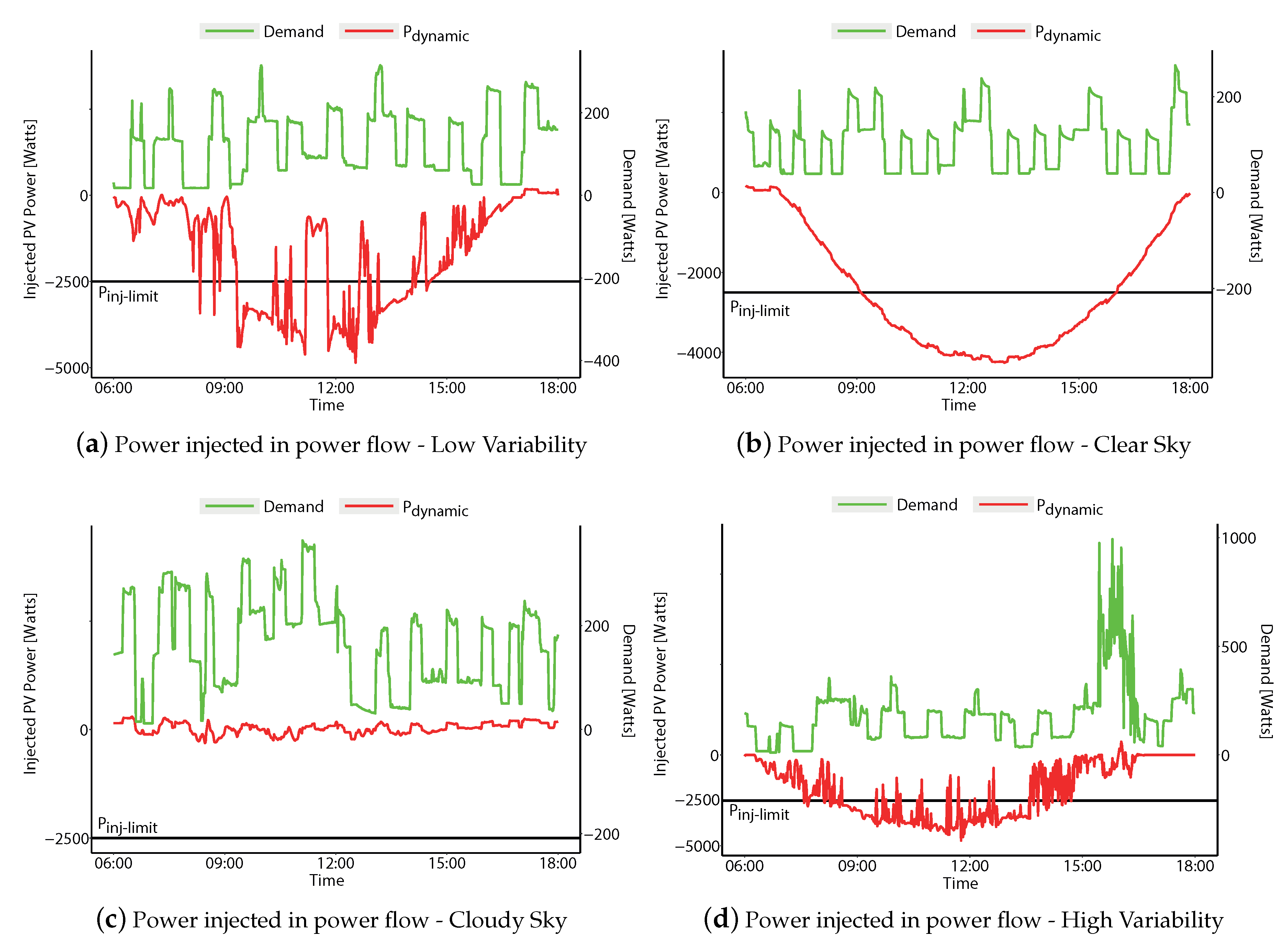
• The mitigation technique proposed in this work was able to reduce voltage levels above the critical limit. For the days of high variability, there was a greater need for energy storage, of 84% more than the day of clear sky, in order to guarantee the mitigation of all points of overvoltage.
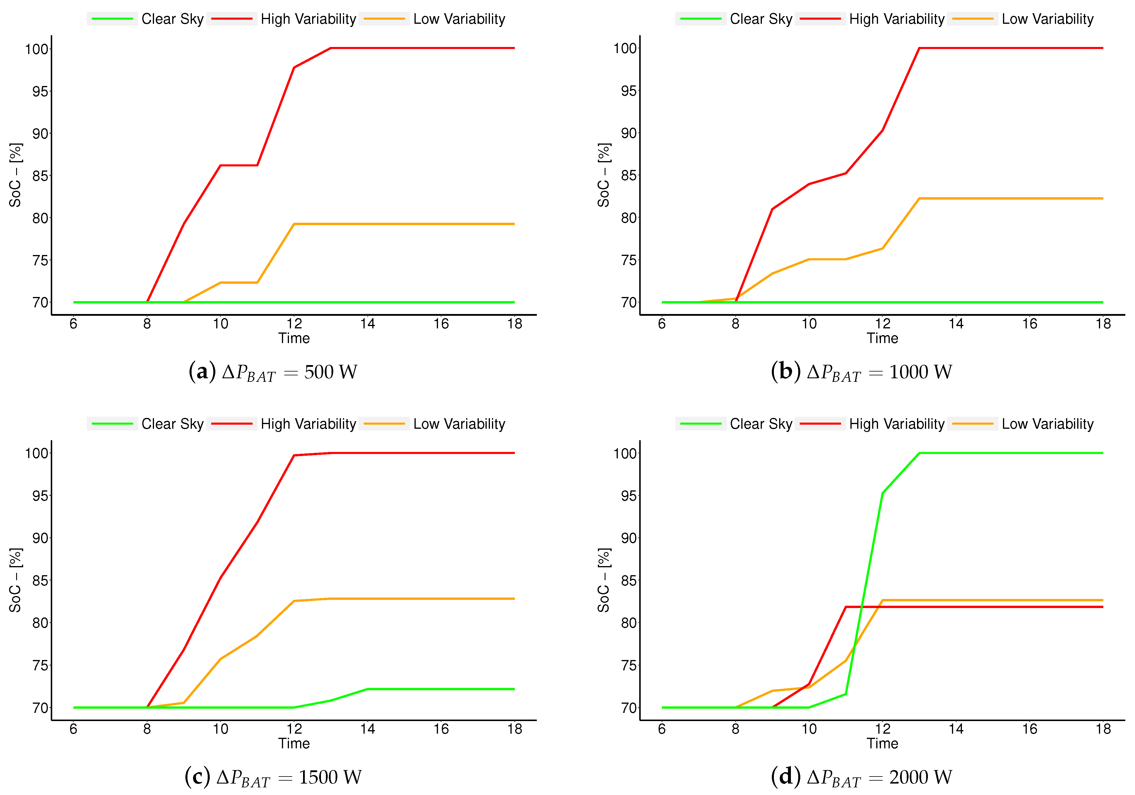
• For a SoC of 70% of the minimum level of total storage capacity, the day of high variability reached full loading of the initial 3 levels of storage. In percentage terms, for $\Delta P_{BAT}=500$ W, $\Delta P_{BAT}=1000$ W, and $\Delta P_{BAT}=1500$ W, it needed supplements of: 252%, 144%, and 134%, respectively, at each level of power. The quantitative percentage is related to the capacity of accumulation of electric energy for the day of low variability.
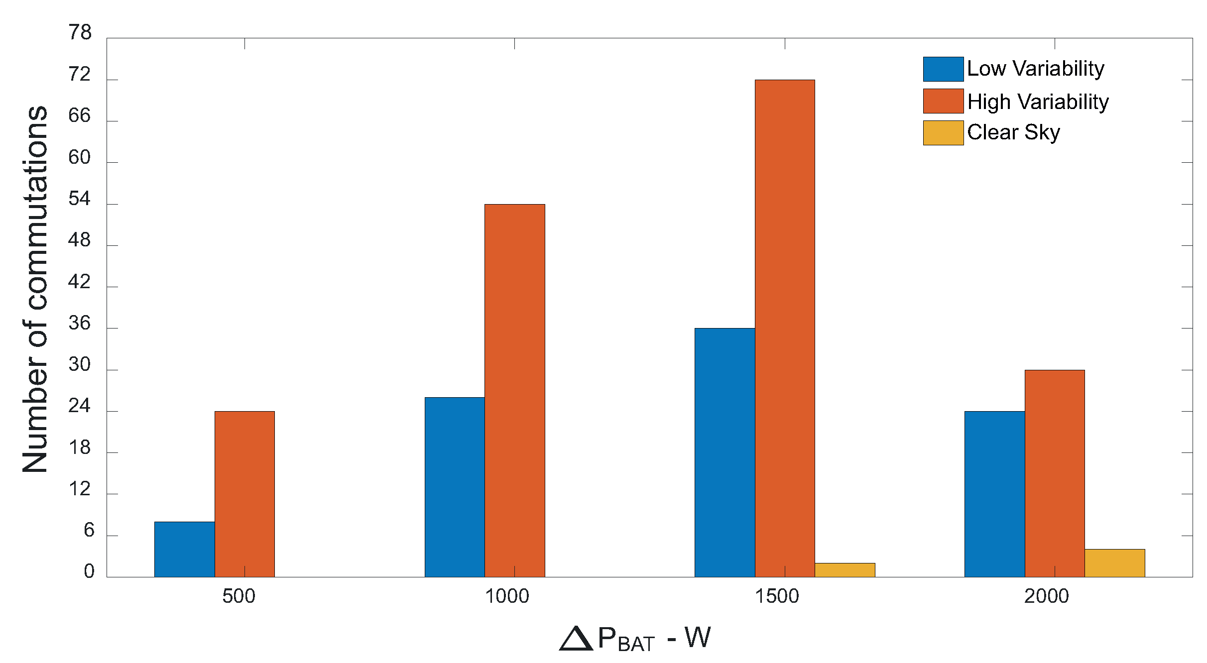
• The number of excessive commutations was classified for the power class $\Delta P=1500$ W, where the number of commutations for the day of high variability was double compared to the day of low variability. The relationship between the number of commutations and accumulated energy was the opposite for the clear day, when looking at the class of power $\Delta P=2000$ W, and this fact is justified by the time that the battery system remained in a state of charge.
• The RNN forecasting model for solar irradiance performed well in the absence of variability, the clear sky, and cloudy sky days presented with a Pearson’s correlation coefficient of 98%. The parameters of RMSE were better for the day of clear sky and cloudy sky, at 47.84 W/m² and 5.69 W/m², respectively. As well as the MAE, for the days of clear sky and cloudy sky, they reached, respectively, 33.44 W/m² and 3.56 W/m². The days characterized as high and low variability showed higher values of RMSE and MAE, as demonstrated throughout the work, concluding with the fact that the neural network had low relative performance for the days with the presence of solar irradiation variability.
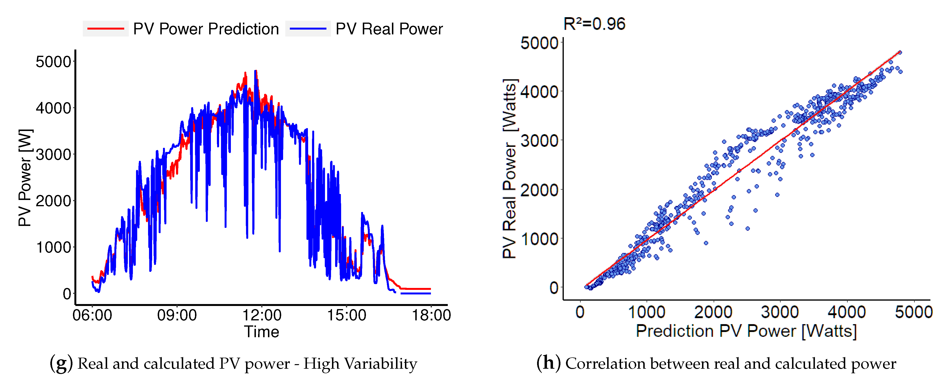
• The model used to calculate the power converted by a photovoltaic generator in the OpenDSS software also presented an excellent profile when compared to the data obtained experimentally. The power flow calculation model based on the irradiation prediction achieved good results for all sky conditions. The days with low and high intermittence were validated with a Pearson’s coefficient of 96% for both days, and the RMSE and the MAE were established in a range of 23.03% and 28.80%, respectively, tolerating the maximum load of the predefined inverter (5000 W).

References

1. Murdock, H.E.; Gibb, D.; André, T. Renewable 2019 Global Status Report. Available online: https://www.ren21.net/wpcontent/uploads/2019/05/gsr_2019_full_report_en.pdf (accessed on 6 January 2020).
2. Bayer, B.; Matschoss, P.; Thomas, H.; Marian, A. The German experience with integrating photovoltaic systems into the low-voltage grids. Renew. Energy 2019, 119, 129–141. [Google Scholar] [CrossRef]
3. Papathanassiou, S.; Hatziargyriou, N.; Anagnostopoulos, P.; Aleixo, L. Capacity of Distribution Feeders for Hosting DER: Report of the International Council of Large Electric Systems. Available online: https://www.cigreaustralia.org.au/assets/ITL-SEPT-2014/3.1-Capacity-of-Distribution-Feeders-for-hosting-Distributed-Energy-Resources-DER-abstract.pdf (accessed on 23 June 2020).
4. Torres, I.C.; Negreiros, G.F.; Tiba, C. Theoretical and Experimental Study to Determine Voltage Violation, Reverse Electric Current and Losses in Prosumers Connected to Low-Voltage Power Grid. Energies 2019, 12, 4568. [Google Scholar] [CrossRef] [Green Version]
5. Marcos, J.; de la Parra, I.; García, M.; Marroyo, L. Control Strategies to Smooth ShortTerm Power Fluctuations in Large Photovoltaic Plants Using Battery Storage Systems. Energies 2014, 7, 6593–6619. [Google Scholar] [CrossRef]
6. Almeida, M.P. Implicações Técnicas da Inserção em Grande Escala da Geração Solar Fotovoltaica na Matriz Elétrica. Ph.D. Thesis, Universidade de Sao Paulo, Sao Paulo, Brazil, 2017. [Google Scholar]
7. Resch, M.; Buhler, J.; Klausen, M.; Sumper, A. Impact of operation strategies of large scale battery systems on distribution grid planning in Germany. Renew. Sustain. Energy 2017, 74, 1042–1063. [Google Scholar] [CrossRef] [Green Version]
8. Chamana, M.; Jahanbakhsh, F.; Chowdhury, B.H.; Parkhideh, B. Dynamic ramp rate control for voltage regulation in distribution systems with high penetration photovoltaic power generations. In Proceedings of the 2014 IEEE PES General Meeting|Conference & Exposition, National Harbor, MD, USA, 27–31 July 2014. [Google Scholar]
9. Zeraati, M.; Golshan, M.E.H.; Guerrero, J.M. Distributed Control of Battery Energy Storage Systems for Voltage Regulation in Distribution Networks With High PV Penetration. IEEE Trans. Smart Grid 2018, 9, 3582–3593. [Google Scholar] [CrossRef] [Green Version]
10. Gevorgian, V.; Booth, S. Technical Requirements for Interconnecting Wind and Solar Generation; National Renewable Energy Laboratory NREL: Golden, CO, USA, 2013.
11. Martins, J.; Spataru, S.; Sera, D.; Stroe, I.D.; Lashab, A. Comparative Study of Ramp-Rate Control Algorithms for PV with Energy Storage Systems. Energies 2019, 12, 1342. [Google Scholar] [CrossRef] [Green Version]
12. Ghaffarianfa, M.; HHajizade, A. Voltage stability of Low-Voltage Distribution Grid with High Penetration of Photovoltaic Power Units. Energies 2018, 11, 1960. [Google Scholar] [CrossRef] [Green Version]
13. Energinet.dk. Techinal Regulation 3.2.2 for a PV Power Plants above 11 kW; Denmark, 2016; Available online: https://en.energinet.dk/Electricity/Rules-and-Regulations/Regulations-for-grid-connection (accessed on 23 June 2020).
14. Campos Filho, M.H.S. Modelagem e Predição de Flutuações da Irradiação Solar de Curta Duração. Ph.D. Thesis, Universidade Federal de Pernambuco, Recife, Brazil, 2019. [Google Scholar]
15. Rabl, A. Active Solar Collectors and Their Applications; Oxford University Press: New York, NY, USA, 1985. [Google Scholar]
16. Carvalho, V.; Barata, H.; Oliveira, W.; Vieira, J.P.A. Impacto da Variabilidade da Geração Fotovoltaica no Controle de Tensão em Redes de Distribuição Ativas. In Proceedings of the XVII Encuentro Regional IBEROAMERICANO de Cigré (ERIAC), CIGRÉ, Ciudad del Este, Paraguay, 21–25 May 2017. [Google Scholar]
17. Alves, M.R.F. O Papel de Geradores Fotovoltaicos na Regulação de Tensão em Redes de Baixa tensãO RESIDENCIAIS: Estudo Comparativo de Normas e Padrões sob a ótica da Mitigação da Elevação de Tensão. Master’s Thesis, Universidade Federal de Minas Gerais, Minas Gerais, Brasil, 2017. [Google Scholar]
18. BORGES, R.T. Desenvolvimento de Metodologias de Análise sistêMica de Sistemas de Distribuição de Energia eléTrica com Geração Ultra-Dispersa. Master’s Thesis, Universidade Estadual de Campinas, Campinas, SP, Brazil, 2014. [Google Scholar]
19. IEEE/CIGRE. Definition and Classification of Power System Stability. IEEE Trans. Power Syst. 2004, 19, 1387–1401. [Google Scholar] [CrossRef]
20. Antonanzas, J.; Osorio, N.; Escobar, R.; Urraca, R.; Martinez-De-Pison, F.J.; Antonanzas-Torres, F. A Review of Photovoltaic Power Forecasting. Solar Energy 2016, 136, 78–111. [Google Scholar] [CrossRef]
21. Wang, F.; Yu, Y.; Zhang, Z.; Li, J.; Zhen, Z.; Li, K. Wavelet decomposition and convolutional LSTM networks based improved deep learning model for solar irradiance forecasting. Appl. Sci. 2018, 8, 1286. [Google Scholar] [CrossRef] [Green Version]
22. Vassalli, L.C. Aplicação de Redes Neurais LSTM para a Previsão de curto Prazo de Vazãodo Rio Paraíba do Sul; Univesidade Federal de Juiz de Fora: Juiz de Fora, Minas Gerais, Brazil, 2018. [Google Scholar]
23. Abdel-Nasser, M.; Mahmoud, K. Accurate photovoltaic power forecasting models using deep LSTM-RNN. Neural Comput. Appl. 2019, 31, 2727–2740. [Google Scholar] [CrossRef]
24. ANEEL; Agência Nacional de Energia Elétrica. Procedimentos de Distribuição de Energia Elétrica no Sistema Elétrico Nacional—Prodist, Módulo 8–Qualidade de Energia Elétrica. v. 10. Disponível em. Brasília. 2017. Available online: https://www.aneel.gov.br/documents/656827/14866914/Módulo_8-Revisão_10/ (accessed on 13 May 2021).
25. ANEEL; Agência Nacional de Energia Elétrica. Resolução Normativa nº 482, de 17 de Abril de 2012. v. 10. Brasília, 2012. Disponível em. Available online: http://www2.aneel.gov.br/cedoc/ren2012482.pdf (accessed on 9 April 2020).
26. Braz, H.D.M. Algoritmos Genéticos para Configuração Ótima de Redes de Distribuição de Energia Elétrica. Master’s Thesis, Universidade Federal de Campina Grande, Campina Grande, Paraíba, Brazil, 2003. [Google Scholar]
27. Oliveira, R.C. Metodologia para o Cálculo de Perdas Técnicas e Não Técnicas de aAlimentadores de Distribuição Via Estudos de Fluxo de Carga pelo Mëtodo Somatório de Potência Modificado. Master’s Thesis, Universidade Federal do Pará, Belém, Pará, Brazil, 2017. [Google Scholar]
28. Lima, R.H.; Bernardon, P.D.; Oliveira, P.H.E. Método de Monte Carlo para Análise de sobretensão m redes secundárias com elevada conexão de Sistemas FV. In Proceedings of the XVII Encuentro Regional IBEROAMERICANO de Cigré (ERIAC), CIGRÉ, Natal, RN, Brasil, 27–30 October 2019. [Google Scholar]
29. Barata, H.A. Impacto de Redes de Distribuição com Massiva Conexão de Geradores Fotovoltaicos na Estabilidade de Tensão de Longo-Prazo em Sistemas de Potência. Master’s Thesis, Universidade Federal do Pará, Belém, Pará, Brazil, 2017. [Google Scholar]
30. Quevedo, J.O. Emprego de um Comutador Eletrônico de Taps para Regulação de Tensão em Redes eléTricas a Partir do Modelo de Carga. Ph.D. Thesis, Universidade Federal de Santa Maria, Santa Maria, Rio Grande do Sul, Brazil, 2018. [Google Scholar]
31. Diaz, V.N. Avaliação do Desempenho das Estratégias de Controle para Suavização da Potência Ativa de Sistemas Fotovoltaicos com Armazenamento de Energia. Master’s Thesis, Universidade Estadual do Oeste do Paraná, Foz do Iguaçu, Brazil, 2019. [Google Scholar]
32. Alzahrani, A.; Ferdowsi, M.; Shamsi, P.; Dagli, C. Solar Irradiance Forecasting Using Deep Neural Networks. Procedia Comput. Sci. 2017, 114, 392–400. [Google Scholar] [CrossRef]
33. Guariso, G.; Nunnari, G.; Sangiorgio, M. Multi-Step Solar Irradiance Forecasting and Domain Adaptation of Deep Neural Networks. Energies 2020, 13, 3987. [Google Scholar] [CrossRef]
34. Chevalier, R.F.; Hoogenboom, G.; Mcclendon, R.W.; Paz, J.A. Support vector regression with reduced training sets for air temperature prediction: A comparison with artificial neural networks. Neural Comput. Appl. 2011, 20, 151–159. [Google Scholar] [CrossRef]
35. Sabino, E.R.C. Previsão de Radiação Solar e Temperatura Ambiente Voltada para Auxiliar a Operação de Usina Fotovoltaicas. Ph.D. Thesis, Tese de Doutorado, Universidade Federal do Pernambuco, Recife, Brazil, 2019. [Google Scholar]
36. Xie, Q.; Shentu, X.; Wu, X.; Ding, Y.; Hua, Y.; Cui, J. Coordinated Voltage Regulation by On-Load Tap Changer Operation and Demand Response Based on Voltage Ranking Search Algorithm. Energies 2019, 12, 1902. [Google Scholar] [CrossRef] [Green Version]
37. Liu, X.; Aichhorn, A.; Liu, L.; Li, H. Coordinated Control of Distributed Energy Storage System With Tap Changer Transformers for Voltage Rise Mitigation Under High Photovoltaic Penetration. Trans. Smart Grid 2012, 3, 897–906. [Google Scholar] [CrossRef]
38. Granzoto, L.M.; Ferreira, S.D.T.; Trindade, F.C.L. Análise dos Transitórios Causados Pela Passagens de Nuvens Sobre Painéis Fotovoltaicos no Número de Atuações de Reguladores de Tensão. In Simpósio Brasileiro de Sistemas Elétricos (SBSE); SBSE: Natal, Brazil, 2016. [Google Scholar]
39. Mahmud, N.; Zahedi, A. Review of control strategies for voltage regulation of the smart distribution network with high penetration of renewable distributed generation. Renew. Sustain. Energy Rev. 2016, 64, 582–595. [Google Scholar] [CrossRef]
40. Ari, G.K.; Baghzouz, Y. Impact of high PV penetration on voltage regulation in electrical distribution systems. In Proceedings of the International Conference on Clean Electrical Power (ICCEP), Ishcia, Italy, 14–16 June 2011. [Google Scholar]
41. Wei, Z.G.; Hu, J.; He, H.; Li, Y.; Xiong, B. Load Current and State of Charge Co-Estimation for Current Sensor-Free Lithium-ion Battery for Voltage Rise Mitigation Under High Photovoltaic Penetration. IEEE Trans. Power Electron. 2021, 3, 1–6. [Google Scholar] [CrossRef]
Figure 1. Typical profile of solar radiation.
Energies 14 03288 g001
Figure 2. Forecast stages.
Energies 14 03288 g002
Figure 3. Forecast stages.
Energies 14 03288 g003
Figure 4. LSTM structure.
Energies 14 03288 g004
Figure 5. Simplified electrical diagram of interconnection of a prosumer to the power grid.
Energies 14 03288 g005
Figure 6. Bidirectional power flow.
Energies 14 03288 g006
Figure 7. Operating voltage limits.
Energies 14 03288 g007
Figure 8. Real representation of the case study.
Energies 14 03288 g008
Figure 9. Proposed method for short-term voltage regulation.
Energies 14 03288 g009
Figure 10. Executive flowchart of the database treatment.
Energies 14 03288 g010
Figure 11. Demand curves measured and a PV cell temperature in the consumer unit equipped with photovoltaic generator.
Energies 14 03288 g011
Figure 12. Steps for creation and operation of the RNN (LSTM) model.
Energies 14 03288 g012
Figure 13. Layout of the electrical circuit representing the storage system and network elements.
Energies 14 03288 g013
Figure 14. Results of predicted radiation compared to actual measured radiation.
Energies 14 03288 g014
Figure 15. Results of the comparison between the operating temperature of the real PV cell and that predicted by the LSTM neural network.
Energies 14 03288 g015
Figure 16. Simulation results (Nowcasted) of the photovoltaic power profiles compared to the measured data.
Energies 14 03288 g016aEnergies 14 03288 g016b
Figure 17. Calculation of the reverse power flow observed by breaking the power allowance limit, showing the demand profile.
Energies 14 03288 g017
Figure 18. Comparison between the rated voltage and the regulated voltage after energy storage.
Energies 14 03288 g018
Figure 19. Total shots for each storage level.
Energies 14 03288 g019
Figure 20. Monitoring of the state of charge (SoC) of the storage system by group of batteries, observing the boundary conditions of solar irradiation.
Energies 14 03288 g020