Abstract
Pakistan’s dependence on energy imports, inefficient power generation and distribution, and lack of planned investment have made the country’s economy vulnerable. Low carbon and resilient climate development in Pakistan can help to ensure climate action and reduce the chronic energy deficit ailing the country’s economy, society, and environment. This study focuses on developing and applying an integrated energy supply-demand modeling framework based on a combination of microeconomics and system integration theories, which can be used to address policies that could dramatically change the future course of Pakistan toward a low emission energy system. The methodology involves medium-term forecasting of energy demand using an integration of top-down and bottom-up modeling approaches. The demand-side model is interlinked with a bottom-up technology assessment supply model. The objective of the supply-side model is to identify the optimal combination of resources and technologies, subject to satisfying technical, institutional, environmental, and economic constraints, using the cost minimization approach. The proposed integrated model is applied to enable a complete perspective to achieve overall reductions in energy consumption and generation and better analyze the effects of different scenarios on both energy demand and supply sides in Pakistan. The results revealed that, in the baseline case, the energy demand is expected to increase from 8.70 Mtoe [106.7 TWh] to 24.19 Mtoe [297.2 TWh] with an annual average growth rate of 6.60%. Increasing the share of renewable energy power generation by 2030 can help to reduce emissions by 24%, which is accompanied by a 13% increase in the total cost of power generation.
1. Introduction
1.1. Background
Through its CO2 emissions in generation and consumption processes, the energy sector is the leading contributor to greenhouse gases (GHGs). According to the United Nations Framework Convention on Climate Change UNFCCC (United Nations Framework Convention on Climate Change), countries signed the Paris Agreement and pledged to reduce their GHG emissions through employing low carbon-based energy generation and efficient consumption [1]. Increasing penetration of renewable energy sources is one of the key target areas for climate mitigation efforts. To access the social, technological, and economic aspects of various strategies for climate mitigation, comprehensive and integrative energy modeling approaches are being employed to help forecast future energy needs and explore different pathways that can help realize emission reduction targets [2].
Sustainable development is about promoting resource and energy efficiency, sustainable infrastructure, and providing access to basic services, green and decent jobs, and a better quality of life for all. It is not just an environmental issue; it is about maintaining the natural capital and hence productivity and capacity of our planet to meet human needs and sustain economic activities. However, unpacking the sustainable development goals (SDGs) that measure Pakistan’s progress on climate action presents a more disconcerting story. SDG 13, “Climate Action”, calls on countries to take immediate action “to combat climate change and its effects”. The United Nations sets out a range of actions and objectives to be taken to achieve SDG 13. A country’s progress in SDG 13 is measured by integrating climate change measures into national policies, strategies, and planning. It is important to recognize that SDG 13 measures Pakistan’s commitment to climate action measures to adopt and implement the National Appropriate National Reduction (NAMA). Pakistan is ranked fifth among countries most vulnerable to the effects of climate change [3] and, even with its minuscule share in global CO2 emissions, is adversely affected by climate change [4].
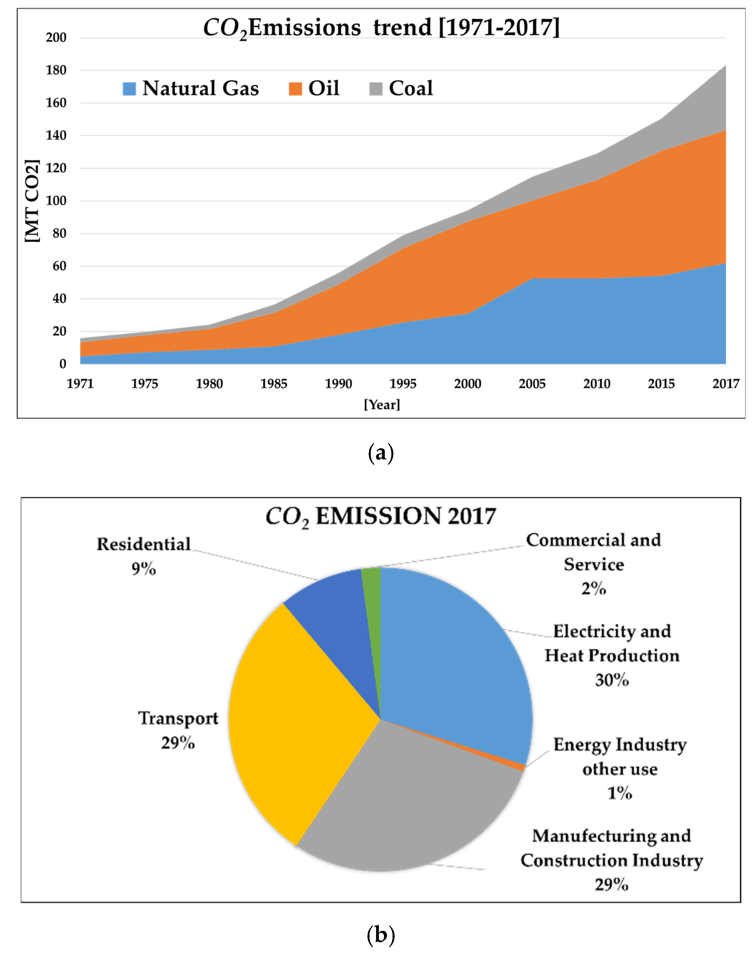
Figure 1 shows the trend of CO2 emissions from fossil fuel burning. To contribute to mitigation efforts, Pakistan ratified the Paris Agreement in 2016 and submitted its National Determined Contribution (NDC) to the UNFCCC with action items to reduce GHGs emissions in various sectors. In the energy sector, renewable energy deployment along with power generation and transmission efficiency are the critical focal points to reduce emissions. Later in 2019, the Alternative Energy Development Board (AEDB) proposed the Renewable Policy 2019 (RE-2019) to substantially increase the renewable shares. It can be observed from Figure 1 that both demand and supply sectors are vital for the analysis to be realized.

Figure 1.
(a) Trends of CO2 emissions from different fossil fuels. (b) Contribution of sectors of the energy system (adapted from [5]).
1.2. Literature Review
Since the last decade, a number of efforts have been made in the context of Pakistan regarding the energy planning and assessment of energy systems under different scenarios. Different methodological methods and tools have been employed to forecast energy demand (demand-side models) and allocate energy supply sources (supply-side models). The demand-side has focused on finding the correlation of energy demand or consumption with economics to quantify the demand factors based on demographic and macroeconomics. Supply-side models have mainly focused on energy supply technologies which are characterized by a limited spatial scale, generally considering a single piece of technology, using an optimization technique to find the optimal energy supply mix. Perwez et al. employed Long-range Energy Alternative Planning (LEAP), an integrated and accounting framework-based energy model, to analyze the power sector within the period of 2011–2030, considering different assumptions for demand policy considerations for the supply system [6]. They projected the future outlook of energy demand and supply under three different scenarios on the supply side, namely BAU (Business-as-usual), NC (New Coal), and GF (Green Future), based on the current trend and future policies on the power sector, especially the National Power Policy 2013. Their results revealed that the GF scenario requires fewer primary resources and provides a cost-effective response to emission restriction. Farooq et al. analyzed the economic and environmental impact of increasing renewable penetration in the future power sector mix for Pakistan for the horizon of 2005–2050 [7]. By employing the Market and Allocation (MARKAL) modeling framework and comparing the results for the different share of renewable energy in their research, they suggested that a 50% share is suitable for Pakistan, and a higher share will become economical. Their results showed that concentrated solar power (CSP) is still not an economically feasible solution for Pakistan. In another effort, Arif et al. developed a comprehensive model to minimize the cost of electricity and emissions for the period 2018–2030 [8]. The model was based on multi-period mix integer programming (MPMIP) and solved by the General Algebraic Modeling System (GAMS), considering three scenarios of fuel switching, fuel balancing, and carbon capture and sequestration (CSS). The Power System Planning department of the National Transmission and Dispatch Company (NTDC) forecasted the future demand for electricity under different economic growth scenarios and then used the Wien Automatic System Planning Package (WASP) model to optimize the future generation expansion plan [9]. The main aim of this study was to encourage energy modeling and planning practices for better power network extensions. Rehman et al. forecasted the future energy demand of all energy carriers for 2015–2035 using three different models of autoregressive integrated moving average (ARIMA), Holt-Winters, and LEAP [10]. Table 1 summarizes the recent studies on employing energy modeling techniques in Pakistan.

Table 1.
Related works on energy modeling in Pakistan.
1.3. Research Gap and Originality Highlights
Despite the diversity of modeling approaches highlighted in Table 1, three challenges exist with all the aforementioned methodologies. The first challenge relates to the methodological foundations of the two categories of demand and supply side, which have usually been developed by focusing on specific aspects of energy use. The second challenge posed by these models is the lack of integration between different demand and supply vectors in the Pakistan energy system, through developing equilibrium-seeking feedback processes, which yields a complex and robust modeling system. The third challenge is to create an analytical framework that explicitly captures some of the linkages between both energy supply and demand sides and other aspects of climate change policies in Pakistan. These challenges can be addressed by the integrated energy supply-demand models, which look at the full set of processes within Pakistan’s whole energy system, enabling a complete perspective to achieve overall reductions in energy consumption and generation and better analyze the direct and indirect effects of policies [24].
This paper aims to develop an integrated energy supply-demand modeling framework based on a combination of the microeconomics and system integration approaches in Pakistan. On the demand side, a combined top-down and bottom-up modeling paradigm is developed for comprehensive analysis of the final energy demand in not only the whole end-use sector, but also in each subsector (transport, electricity, residential, and service), considering the impacts of various scenarios for deploying patterns of efficient use of energy. The energy demand is then defined as a function of its main determinant drivers (i.e., population, dwelling size, floor area, traveled distance, etc.) and can be estimated by the demand-side model, which is interlinked to a bottom-up technology assessment supply model. The objective of the supply energy model is the minimization of the total cost of meeting exogenously specified levels of energy demand. The primary strength of the proposed modeling approach in this study is its integrated approach to produce reliable and policy-sensitive forecasts that retain the link between different demand and supply vectors in the energy system in Pakistan.
The remainder of this paper is organized as follows: the demand and supply modeling framework is explained in Section 2. Section 3 covers the details about data settings. Section 4 includes the detailed scenario definition. Section 5 covers the results and discussions. The final section concludes the paper with policy recommendations.
2. Model Development
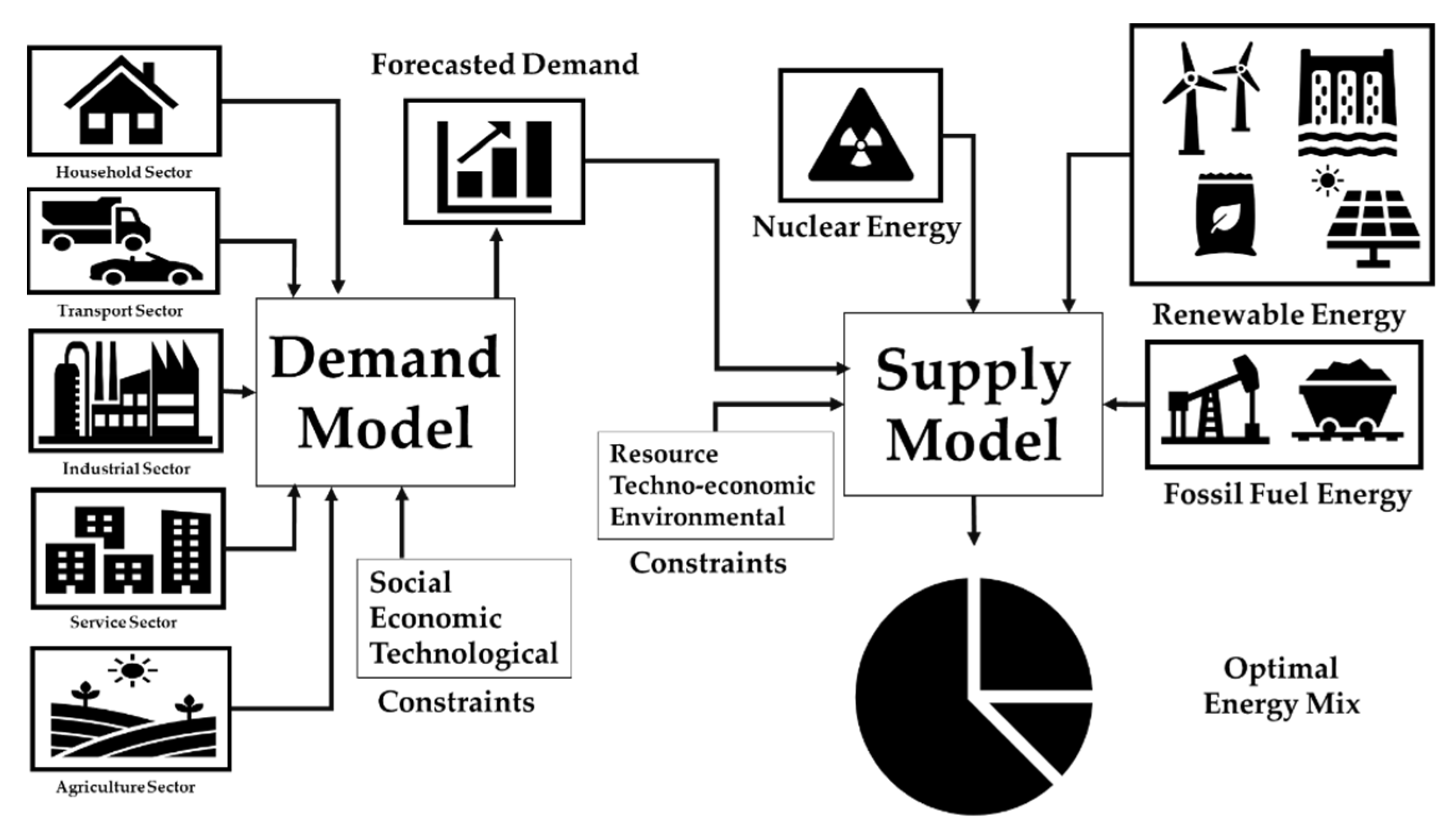
The analysis of the Pakistan energy system should be used to suggest appropriate energy and environmental policy to sustain economic growth and improve the environmental quality for better living standards in the country. This entails that a tradeoff between the efficient use of energy, including environmental quality, and sustained economic growth in the long term. Hence, in this study, the main focus is developing an integrated modeling framework that can explicitly consider the impact of macro- and microeconomics and the reinvestment of the additional capacity requirement on the supply-demand match in the Pakistan energy system. Based on this idea, the overall framework of the integrated energy modeling concept was developed, which is presented in Figure 2. First, considering the characteristics, demand factors, and future scenarios of different sectors, the demand model will project future energy demand on a disaggregated level. Total energy demand in Pakistan is considered as a function of the energy price, income, and sectoral gross value added (GVA). Second, the macrolevel energy demand analysis is followed by a detailed microlevel analysis through segregating the whole energy system to its main sectors, such as household, commercial, industrial, service, and agriculture sectors. This involves a bottom-up assessment which relates the specific energy demand in different sectors systematically to the corresponding social, economic, and technological factors that affect this demand. Finally, the supply model then uses this demand to optimize the energy mix, considering the technical and economic aspects of technologies, resource availability, and environmental considerations.

Figure 2.
The overall concept of an integrated energy model for Pakistan.
2.1. Demand-Side Model
2.1.1. Top-Down Econometric-Based Demand Model
Econometrics applies macroeconomic theories on the historical data to quantify the impact of economic factors, such as energy price, income, sectoral gross value added (GVA), etc., on energy demand and project future demand. Figure 3 shows the framework adopted for quantifying the factors of energy demand in this study. The unit root test verifies the stationarity of time series data. Multiple regression for the nonstationary data may generate a spurious regression that leads to unreliable results. Autoregressive and distributed lag (ARDL) takes into account sufficient lags of variables to avoid nonstationarity [25,26,27]. The Durbin–Watson test is used to verify the reliability of the analysis. If the Durbin–Watson test is failed, the demand models are revisited to find the suitable combination and form (i.e., variables in log form).
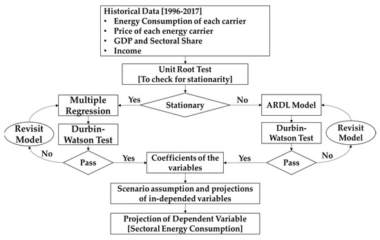
Figure 3.
The framework of the econometric analysis of demand in this study.
The following equation shows the standard representation of the ARDL model [28]:
where and are explanatory and explaining variables, respectively; and are the order of lags for respective variables; is the constant term; and are the coefficient of lagged explanatory and explaining variables, respectively; and is the error term. The combination of sectoral energy consumption, energy price, income, and sectoral value added for different sectors is summarized in Table 2.

Table 2.
Macroeconomic parameters used in the econometric model.
The income and GVA were correlated with GDP using the similar ARDL approach, and future projections were subjected to the growth rate of GDP and sectoral share of the economic sector. Energy price was correlated to the inflation rate to quantify the contribution of energy price towards the overall consumer price index (CPI).
2.1.2. Bottom-Up Simulation-Based Demand Model
The bottom-up model is based on the simulation approach, which forecasts the future energy demand, considering the economic, social, and technological aspects related to energy demand. The following is the elaboration of the key terms:
- ○
- The social aspects include the parameters population, household characteristics, and lifestyle.
- ○
- The economic aspect deals with the level of the activity in economic sectors or subsectors.
- ○
- The technological aspect is based on selecting different available technologies (fossil fuel, electricity, renewable and traditional fuel), taking into account their efficiency and market penetration.
The bottom-up energy demand is segregated into five main sectors: industry, transportation, household, agriculture, and service. These sectors, where applicable, are further divided into subsectors or end-use categories to include the impact of disaggregation. The model first calculates the useful energy respect of fuel and consumption technology. Then, based on the efficiency and market penetration of different technologies and fuels, demand is estimated and segregated into electric and nonelectric energy demand. Figure 4 represents the framework of the bottom-up energy demand model.
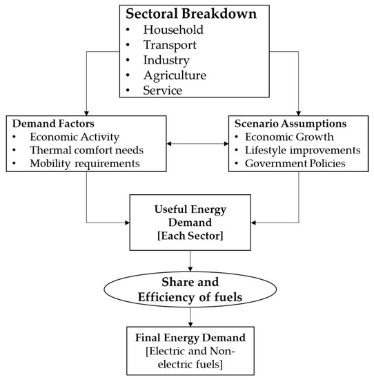
Figure 4.
The framework of the bottom-up energy demand model.
Activity and energy intensity of any sector/sub-sector are the main factors for energy demand simulation. Table 3 shows the definition of activity for different sectors and subsectors. The total amount of energy consumption can be estimated from the multiplication of energy intensity to the unit of activity for each sector.

Table 3.
Definition of the terms of activity in the bottom-up energy demand.
Considering the above definition for activity, the following is the general representation of the calculation of energy demand for each sector [29]:
where is the useful energy demand of sector; , , and represent the activity, share, and energy intensity (specific energy requirement), respectively, for each subsector; and final energy demand for any fuel is calculated using its share and efficiency .
The following are the detailed equations for different sectors of the bottom-up energy demand model.
Household Sector:
Space Heating:
Air Conditioning and Electrical Appliance:
Water Heating and Cooking:
is the useful energy demand for space heating [kWh]. is the total number of dwellings of type , share (%) , and size (sqm) . HDD is heating degree days, and is the effective heating area (%). is the heat loss from different dwelling types [kWh/°C m2h]. is the energy demand for air conditioning and other electric appliances [kWh]. is the ownership, i.e., percentage of households having facility of the specific appliance. is the quantity of appliance per dwelling, and is the energy intensity [kWh/unit/year]. is the useful energy demand for the water heating and cooking subsectors [kWh]. It is calculated by using the household size (number of persons/household) and per capita energy consumption [kWh/cap]. is the dwellings having the facility of water heating.
Transport Sector [29]:
For passenger transport energy demand ), is total passenger kilometer, and and are the share [%] and energy intensity [GJ/PKM] of vehicle category with fuel . For freight transport energy demand ), ton-kilometer ( is used instead of .
Economic Sectors:
For economic sectors (industry, service, and agriculture), is gross value added of these sectors [$], and and reprensent the share [%] in value added and energy intensity [kWh/$] for each subsector, respectively.
2.2. Energy Supply Model
After computation of demand for all the sectors for the model horizon, the next step is to use the energy supply model to optimally allocate different energy sources to meet the demand. In this study, the Model for Energy Supply Systems and their General Environmental Impact (MESSAGE) is used as the energy supply model, based on the flexibility of scenarios and comprehensive analysis approach [30]. The MESSAGE model involves a detailed representation of technical engineering, socioeconomic, and biophysical processes in energy and land-use systems, aiming to satisfy a given demand level at the least cost. Figure 5 represents the flow chart describing the process of MESSAGE modeling.
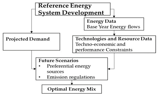
Figure 5.
Framework of MESSAGE energy model.
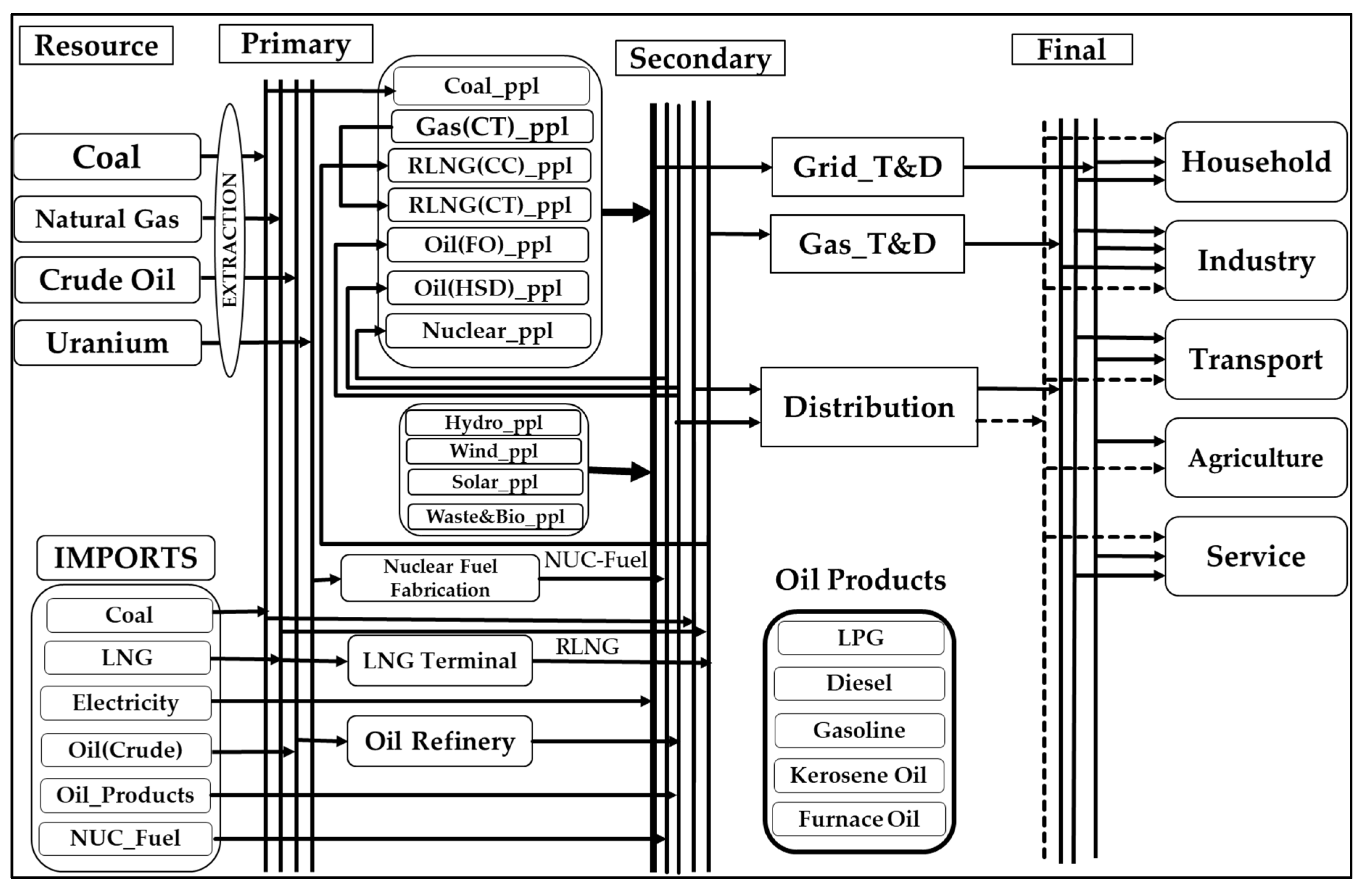
Figure 6 shows the reference energy system (RES) in Pakistan developed in the MESSAGE model. This reference system shows the different levels of the energy system and the linkage among the various energy conversion, processing, transmission, and distribution technologies.

Figure 6.
Reference Energy System (RES) for Pakistan.
The model is based on the minimization of the total discounted cost of the energy system. The cost variable represents the total cost of the resource, investment for new technology, operation and maintenance, and emissions, as follows:
where DR is the discount rate; y is year; and is the total cost for year y. and are cost and extracted resources of each type and grade . , , and represent the investment, fixed, and variable costs for each technology , whereas , , and are the additional, maintained capacities and energy flow, respectively. represents the activity level of each technology, which, here, is considered as the energy outflow from the technology. and are the emission tax and emission amount for each technology and emission category .
The objective function, the total cost, is constrained to the number of technical, economic, environmental, and resource constraints. The following equations represent the main constraints of the model:
- Demand constraint:where is the given level of the energy demand of any energy carrier ; at level for each load region, must be met by the total energy flows of all the technologies feeding that level in each year .
- Capacity constraint:
The activity level of each technology under the operation mode is constrained by the duration of the lead region , its capacity factor , and maintained capacity during the year.
- 3.
- Resource constraint:
The extraction of resource during a year must be lower the resource volume and extracted during the previous year by the rate of extraction of the remaining resource in each year.
Focusing on the intermittence nature, renewable sources, especially solar and wind, are prone to high risk in the reliable operation of the power system. The reliability of the power system depends upon two main factors, capacity reserve and flexibility. The capacity reserve ensures that the system has enough generation capability to meet the maximum load demand under normal and contingent conditions. Flexibility means how quickly the generation system can respond to sudden changes in load. Hence, the overall purpose of system reliability is that the supply system must meet the demand at all levels and at all times.
For conventional power generation sources, reserve capacity requirements can be evaluated by the nominal capacity and reliability factor (calculated based on the probability of forced outage). In the case of wind- and solar-based generation, nameplate rating cannot ensure the required contribution to capacity reserve because of their variable nature. In this situation, the MESSAGE model employs the capacity values for solar and wind power plants according to the share in load [31].
Employing the analysis discussed in Sullivan et al. [31], the flexibility of different power plants and associated technologies is quantified as a factor ranging from −1 to 1. The positive sign is used for the technologies that can provide flexibility, and the negative is used for the technologies that require additional flexibility for integration with the power system. The magnitude of the factor shows the extent of this flexibility. Table 4 shows the flexibility factors of technologies involved in this study. Minimal and negative values for wind and solar power plants show that they require flexibility from conventional flexible sources, especially gas, high-speed diesel (HSD), and hydro-based power plants or electric storage.

Table 4.
The flexibility factors used in the MESSAGE model in this study.
2.3. Integration of Demand-Supply Models
The top-down econometric-based model is used for the future projection of total sectoral energy demand. The bottom-up energy demand model disaggregates this demand into different fuels by adjusting its assumption and considering the efficiency and market penetration of energy carriers. Finally, this demand is given to the MESSAGE model to optimize the supply mix (see Figure 7).
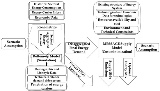
Figure 7.
Integration of demand and supply models in this study.
3. Data Inventory
Annual Energy Yearbooks (EYB) published by the Hydrocarbon Development Institute of Pakistan (HDIP) are the main sources of data on energy consumption, energy prices, resource cost and reserve details, and the activity of different energy conversion technology (i.e., power plants, oil refineries, gas processing plants) [32]. The economic and social data are collected from the World Bank [28], Economic Survey of Pakistan [29], and Pakistan Bureau of Statistics (PBS) [30].
3.1. Top-Down Energy Demand Data
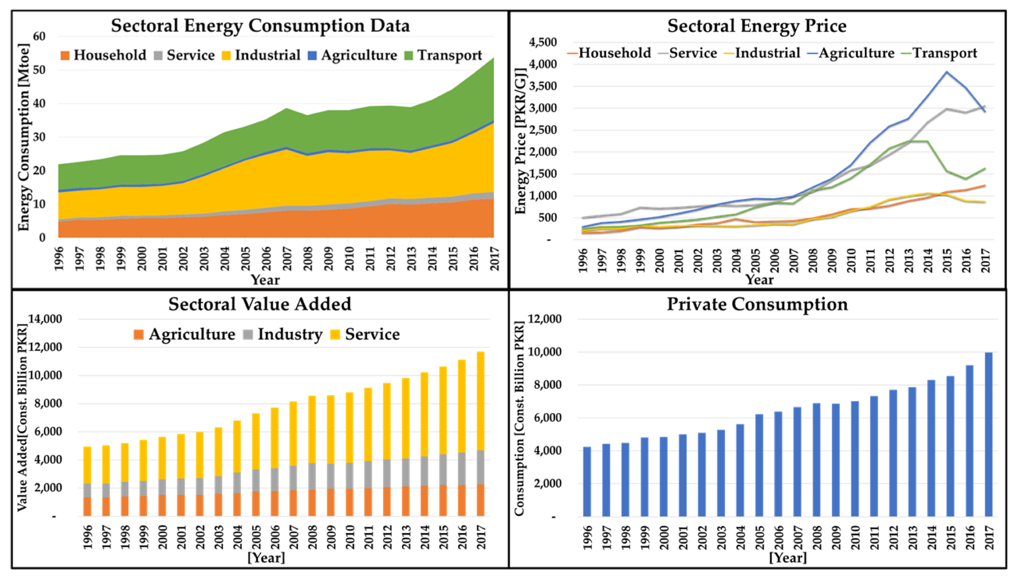
All energy-related data for this analysis section is collected from the various editions of the Energy Yearbook from HDIP [32]. Energy consumption data is disaggregated into different fuels in five sectors. The prices of fuels, especially electricity and natural gas, are updated nonuniformly throughout the year. For the yearly analysis, the time-weighted average is calculated for both of these carriers. Moreover, the overall sectoral energy price was computed using the energy consumption weighted average of the price of fuels. Due to the unavailability of household income at a yearly frequency, the data on private consumption is referred to as a proxy for income. The data on private consumption, sectoral, and overall value added is collected from the World Bank Development Indicators [33]. Real prices were calculated using the GDP deflator, referred to as World Bank Development Indicators [33]. Table 5 shows the descriptive analysis of the involved time series data in log form for econometric analysis. Figure 8 represents the historical data (1996–2017) on the abovementioned data.

Table 5.
Descriptive analysis of variables (in log form) for econometric analysis.

Figure 8.
Timeseries data of parameters used in top-down energy demand model.
3.2. Bottom-Up Energy Demand Data
The data on household characteristics, ownership of electric appliances, and fuel choices were adapted from the Pakistan Social and Living Standards Measurement (PSLM) and the Household Integrated Economic Survey (HIES) periodical conducted by the Pakistan Bureau of Statistics (PBS) [34]. The Pakistan National Census 2017 conducted by PBS [35] is referred to as the latest data for urban and rural populations, the number of households, and the share of the urban population. The future trends of the population were collected from the medium-variant projection made by United Nations Report [36]. The Economic Survey of Pakistan [37] was used for collecting required data (i.e., vehicle population for different categories) in the transport sector. The data used in the bottom-up assessment of the energy demand in different subsectors are given in Table 6, Table 7, Table 8, Table 9, Table 10 and Table 11.

Table 6.
Basic demographic data [35].
In this study, the households are categorized into small, medium, and large, assuming the common area of household in local units to be 3 marla (76 sq.m), 5 marla (126 sq.m), and 7 marla (177 sq.m), respectively. The effective area for heating is calculated on the basis of the area of the standard room size of 9.3 sq.m. The heat losses were calculated using the Building Codes of Pakistan 2017 [38]. The heating degree days (HDD) values are calculated from [39].

Table 7.
Characteristics of different household categories [34,35,38,40,41,42].
Table 7.
Characteristics of different household categories [34,35,38,40,41,42].
| Parameter | Unit | Urban | Rural | ||||
|---|---|---|---|---|---|---|---|
| Small | Medium | Large | Small | Medium | Large | ||
| Dwelling Share | [%] | 24.87 | 69.25 | 5.89 | 30.4 | 64.4 | 5.2 |
| Total Area of Dwelling | [sqr. m] | 76 | 126 | 177 | 126 | 177 | 253 |
| Effective Area for Space Heating | [%] | 12 | 22 | 32 | 11 | 23 | 32 |
| Heat Loss | [Wh/sqm/°C/h] | 0.54 | 0.53 | 0.53 | 0.54 | 0.53 | 0.53 |
| Share of Dwelling Having AC Facility | [%] | 21.7 | 21.7 | 21.7 | 3.8 | 3.8 | 3.8 |
| Specific Energy for Cooking | [kWh/cap/yr] | 2728 | 2728 | 2728 | 2728 | 2728 | 2728 |
| Specific Energy for Water Heating | [kWh/cap/yr] | 110 | 110 | 110 | 110 | 110 | 110 |
| Share of Dwelling with Hot Water Facility | [%] | 77 | 77 | 77 | 42 | 42 | 42 |

Table 8.
Ownership and energy requirement details of electric appliances and the share of different fuels and household sectors [32,34].
Table 8.
Ownership and energy requirement details of electric appliances and the share of different fuels and household sectors [32,34].
| Home Appliance | Dwelling Type | Urban [%] | Rural [%] | Units | Wattage | Usage (Day/yr) | Usage (hrs/Day) |
|---|---|---|---|---|---|---|---|
| Air Conditioner | Small | 21.7 | 3.8 | 1 | 1460 @ 75% | 120 | 4 |
| Medium | 21.7 | 3.8 | 1 | 1950 @ 75% | 120 | 4 | |
| Large | 21.7 | 3.8 | 2 | 1950 @ 75% | 120 | 5 | |
| Television | All | 86.4 | 48.1 | 1 | 100 | 365 | 5 |
| Refrigerator | All | 77.1 | 41.9 | 1 | 220 | 365 | 6 |
| Room Cooler | All | 25.1 | 11.2 | 1 | 185 | 180 | 8 |
| Washing Machine | All | 82.9 | 44.4 | 1 | 500 | 53 | 2 |
| Water Pump | All | 68.3 | 46.8 | 1 | 380 | 365 | 1 |
| Fan | All | 99.4 | 95.9 | 3 | 60 | 300 | 8 |
| Lights | All | 99.4 | 95.9 | 5 | 40 | 365 | 4 |
| Fuel | Urban [%] | Rural [%] | |||||
| Space Heating | Water Heating | Cooking | Space Heating | Water Heating | Cooking | ||
| Biomass | 11.71 | 11.71 | 11.71 | 81.33 | 81.33 | 81.33 | |
| Electricity | 2.0 | 2.0 | 2.0 | 2.0 | 2.0 | 2.0 | |
| Solar | 0 | 0 | 0 | 0 | 0 | 0 | |
| Fossil Fuel | 86.3 | 86.3 | 86.3 | 16.7 | 16.7 | 16.7 | |
| Share | Natural Gas | LPG | Kerosene | ||||
| Fossile Fuel [%] | 91.7 | 0.94 | 7.39 | ||||
Car ownership (number of cars per 1000 persons) is computed using population and on-road cars [33,37]. The rest of the parameters in Table 9 are calculated for the given demand of energy consumption in the transport sector [32].

Table 9.
Basic information related to passenger and freight activities.
Table 9.
Basic information related to passenger and freight activities.
| Parameter | Unit | Value |
|---|---|---|
| Intracity Distance Travelled | [km/prsn/day] | 38.17 |
| Intercity Distance Travelled | [km/prsn/yr] | 13931 |
| Car Ownership | [person/car] | 25.47 |
| Intercity Car-km | [km/car/yr] | 4000 |
| Freight ton-km (TKM) | [109 tkm] | 349.6 |

Table 10.
Detail of passenger and freight transport [37,43,44].
Table 10.
Detail of passenger and freight transport [37,43,44].
| Subsector | Vehicle Category | Vehicle Type | Modal Share [%] | Load Factor [person/vehicle] | Fuel Type | Share by Fuel | Energy Intensity |
|---|---|---|---|---|---|---|---|
| [%] | [l/100 km] * | ||||||
| Intercity Passenger Transport | Private | Car | - | 2.6 | Gasoline | 82 | 9.1 |
| Diesel | 10.5 | 10 | |||||
| CNG | 7.5 | 8.1 | |||||
| Electricity | 0 | 16.5 | |||||
| Public | Vans | 35.72 | 12 | Gasoline | 100 | 5 | |
| CNG | 0 | 5.61 | |||||
| Bus | 47.2 | 50 | Diesel | 100 | 28.6 | ||
| Train | 17.1 | - | Diesel | 100 | 3.1 | ||
| Intracity Passenger Transport | Private | Car | 37.06 | 2.6 | Gasoline | 82 | 9.1 |
| Diesel | 10.5 | 10 | |||||
| CNG | 7.5 | 8.1 | |||||
| Electricity | 0 | 16.5 | |||||
| 2 Wheelers | 47.21 | 1.6 | Gasoline | 100 | 2.5 | ||
| Electricity | 3.3 | ||||||
| Public | Taxi | 2.91 | 2.6 | Gasoline | 91.6 | 7.1 | |
| CNG | 8.37 | 6.4 | |||||
| Electricity | 0 | 13.3 | |||||
| 3 Wheelers | 1.82 | 1.8 | Gasoline | 91.6 | 4.55 | ||
| CNG | 8.37 | 8.1 | |||||
| Electricity | 0 | 6.1 | |||||
| Vans | 5.79 | 12 | Gasoline | 91.6 | 5 | ||
| CNG | 8.37 | 5.61 | |||||
| Bus | 5.21 | 50 | CNG | 100 | 23.14 | ||
| Frieght Transport | - | Pickup | 5.2 | - | Diesel | 100 | 6.7 |
| Truck | 91.6 | Diesel | 100 | 2.3 | |||
| Train | 3.24 | - | Diesel | 100 | 2.3 |
* For electric fuels, passenger trains, and freight transport, the units of energy intensity are kWh/100 km, kWh/100 pkm, and l/100 tkm, respectively.

Table 11.
Economic sectors details [32,33].
Table 11.
Economic sectors details [32,33].
| Economic Sector | Value Added [Tr. PKR] | Share in GVA [%] | Energy Intensity [kJ/PKR] | Share of Fuels [%] | ||||
|---|---|---|---|---|---|---|---|---|
| Oil | Natural Gas | Coal | LPG | Electricity | ||||
| Agriculture | 2.25 | 19.3 | 15.6 | 1.8 | - | - | - | 98.2 |
| Industry | 2.43 | 20.8 | 355.1 | 8.87 | 37.9 | 42.1 | - | 11.1 |
| Service | 7.01 | 60.0 | 12.0 | - | 37.4 | - | 27.76 | 34.9 |
3.3. Energy Supply Data
The input data for the MESSAGE model involves the technical details and limitation of technologies, resource availability and cost, emission factors, and energy balance for the base year, which are given in Table 12, Table 13, Table 14 and Table 15.

Table 12.
Technical details and base year status of technologies [9,32].
Table 12.
Technical details and base year status of technologies [9,32].
| Parameters | Efficiency [%] | Capacity Factor [%] | Operation Factor [%] | Reliability Factor [%] | Aux. Power [%] | Base Year Generation [GWa] | Base Year Capacity [GW] | Min. Utilization [%] |
|---|---|---|---|---|---|---|---|---|
| Coal(IMP)_ppl | 39.04 | 100 | 92 | 93 | 0.03 | 1.24 | 2.84 | 25 |
| Coal(LOC)_ppl | 39.04 | 100 | 92 | 93 | 0.03 | 0.00 | 0.03 | 0 |
| Gas_ppl | 34.39 | 100 | 89 | 95 | 2.58 | 3.10 | 8.01 | 50 |
| RLNG(CT)_ppl | 34.39 | 100 | 89 | 95 | 2.58 | 1.40 | 4.02 | 50 |
| RLNG(CC)_ppl | 55.69 | 100 | 89 | 95 | 2.58 | 1.12 | 3.67 | 50 |
| Oil(FO)_ppl | 38.77 | 100 | 92 | 95 | 5.48 | 3.28 | 8.42 | 50 |
| Oil(HSD)_ppl | 33.77 | 100 | 92 | 95 | 2.01 | 0.09 | 0.13 | 50 |
| Nuclear_ppl | 36.75 | 100 | 84 | 95 | 7.12 | 1.13 | 1.47 | 80 |
| Hydro_ppl | 100 | 50 | 97 | 93 | 0.81 | 3.19 | 8.72 | 0 |
| Wind_ppl | 100 | 32.76 | 97 | 100 | 0 | 0.24 | 1.05 | 0 |
| Solar_ppl | 100 | 21 | 100 | 100 | 0 | 0.09 | 0.43 | 0 |
| Waste&Bio_ppl | 100 | 57 | 97 | 93 | 0 | 0.11 | 0.42 | 0 |

Table 13.
Cost and environmental parameters of power technologies [9,32,45].
Table 13.
Cost and environmental parameters of power technologies [9,32,45].
| Parameters | Plant Life [Years] | Construction Time [Years] | Investment Cost [$/kW] | Investment Cost Reduction [%] | Fix. Cost [$/kW-Year] | Var. Cost [$/kWa] | Emission Factor [MT CO2/GWa] |
|---|---|---|---|---|---|---|---|
| Coal(IMP)_ppl | 40 | 4 | 1556 | 0.30 | 25.56 | 32.32 | 6.31 |
| Coal(LOC)_ppl | 40 | 4 | 1556 | 0.30 | 173.28 | 61.32 | 6.31 |
| Gas_ppl | 30 | 2 | 534 | 0.54 | 19.2 | 16.64 | 4.53 |
| RLNG(CT)_ppl | 30 | 2 | 534 | 0.54 | 19.2 | 16.64 | 4.53 |
| RLNG(CC)_ppl | 30 | 2 | 694 | 0.59 | 17.16 | 31.19 | 4.53 |
| Oil(FO)_ppl | 40 | 4 | 694 | 0.00 | 55 | 6.48 | 5.96 |
| Oil(HSD)_ppl | 30 | 4 | 534 | 0.00 | 36 | 9.63 | 6.68 |
| Nuclear_ppl | 40 | 7 | 4342 | 0.54 | 71.76 | 17.52 | 0.00 |
| Hydro_ppl | 50 | 5 | 2488.4 | 0.00 | 13.16 | 36.79 | 0.00 |
| Wind_ppl | 50 | 2 | 2500 | 1.78 | 25.48 | 0.00 | 0.00 |
| Solar_ppl | 30 | 2 | 1300 | 1.80 | 40.82 | 0.00 | 0.00 |
| Waste&Bio_ppl | 30 | 2 | 4000 | 0.30 | 109.01 | 47.55 | 3.50 |
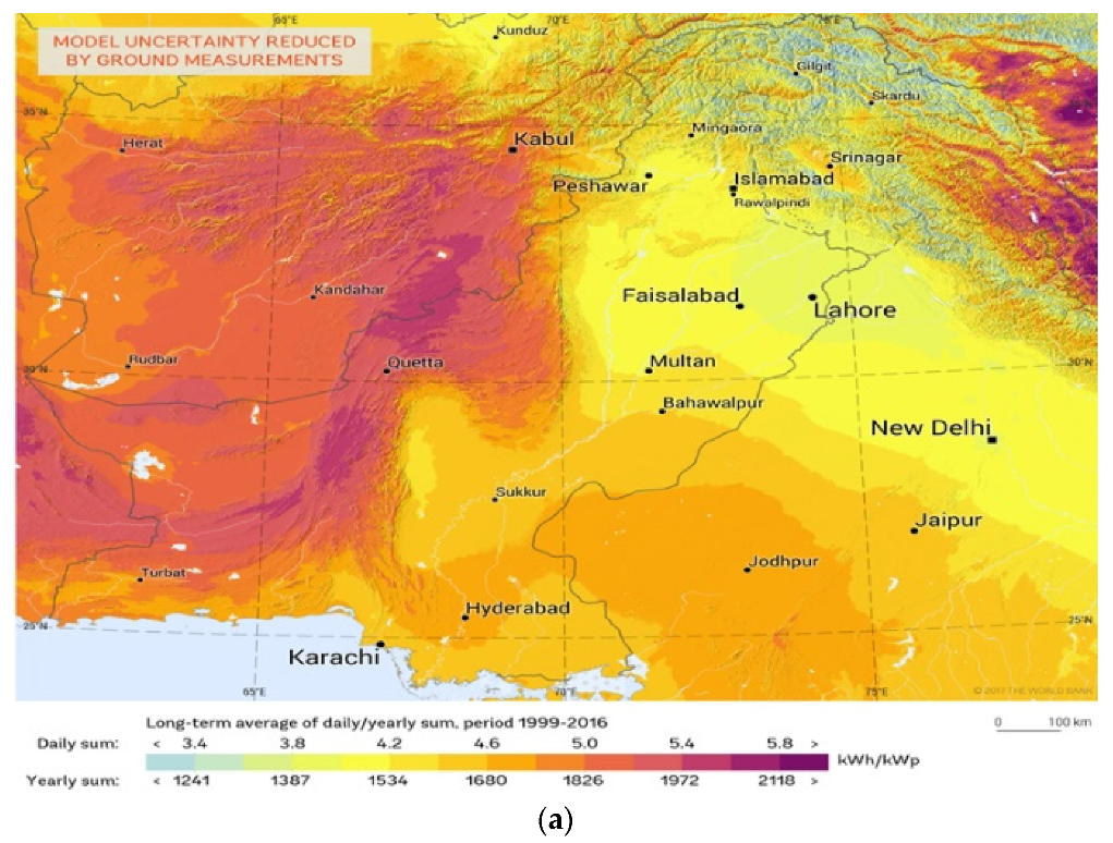
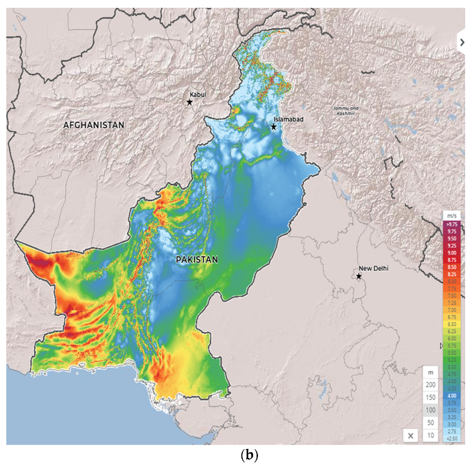
Coal is the leading reserve in Pakistan with limited extraction. The government has started the extraction of domestic coal for power generation use and will lower the extraction of natural gas resources in the next few years. Crude oil has already crossed its peak. On the renewable energy side, Pakistan is blessed with immense potential, especially solar and wind. Being an agriculture-based country, hydro is the most explored and promising renewable resource. Figure 9 shows the potential map for solar and wind energies in Pakistan. The resource availability in Pakistan and energy imports are given in Table 14 and Table 15.

Table 14.
Resource cost and availability data [9,32,46,47].
Table 14.
Resource cost and availability data [9,32,46,47].
| Category | Resource | Reserve | Cost | Base Year Extraction | |||
|---|---|---|---|---|---|---|---|
| Unit | Value | Unit | Value | Unit | Value | ||
| Fossil Fuel | Coal | [MT] | 7779.8 | [$/T] | 19.1 | [MT/Year] | 4.3 |
| Natural Gas | [BCF] | 20958.9 | [$/MCF] | 5.1 | [BCF/Year] | 1166.0 | |
| Crude Oil | [MT] | 51.1 | [$/T] | - | [MT/Year] | 4.4 | |
| Uranium | [T] | 33,288.0 | [$/kg] | 360.0 | [T/Year] | 45.0 | |
| Renewables | Hydro | [GW] | 40 | - | - | - | - |
| Wind | [GW] | 120 | - | - | - | - | |
| Solar | [GW] | 2900 | - | - | - | - | |
| Waste and Bio | [GW] | 4.068 | - | - | - | - | |

Table 15.
Cost and quantity of imports [9,32].
Table 15.
Cost and quantity of imports [9,32].
| Commodity | Imports | Cost * | ||
|---|---|---|---|---|
| Unit | Value | Unit | Value | |
| Electricity | [GWa] | 0.06 | [$/kWa] | 587 |
| Crude Oil | [MT] | 10.33 | [$/T] | - |
| High-Speed Diesel [HSD] | [MT] | 3.85 | [$/T] | 892 |
| Petrol | [MT] | 5.01 | [$/T] | - |
| Furnace Oil | [MT] | 5.87 | [$/T] | 555 |
| LNG | [BCF] | 320.18 | [$/MCF] | 12.5 |
| Coal | [MT] | 13.68 | [$/T] | 131 |
| Nuclear Fuel | [T] | 19.10 | [$/kg] | 2830 |
| LPG | [MT] | 0.40 | [$/T] | - |
* Only power generation-related costs are considered.
3.4. Main Assumptions for Demand and Supply Models
The following are the main assumptions used in developing the energy demand and supply models.
- Local and imported coal have a share of 77.3% and 22.7% in total final energy demand, respectively.
- The peak demand factor (ratio of annual peak load to average yearly load) for electricity is about 2.19 [9] and is assumed to be constant throughout the model horizon.
- Air conditioning and electric appliances are the major consumers of electricity in buildings.
- The future anticipated domestic natural gas production is estimated based on the Oil and Gas Regulatory Authority (OGRA) [48].
- For coal extraction, the maximum production is assumed to be increased at an annual growth rate of 40% with respect to the base year as planned in Pakistan Vision 2025 [49].
- Extraction of domestic natural uranium is limited to 45 T/year.
- The resource cost and imported fuel prices are assumed to be constant throughout the model horizon.
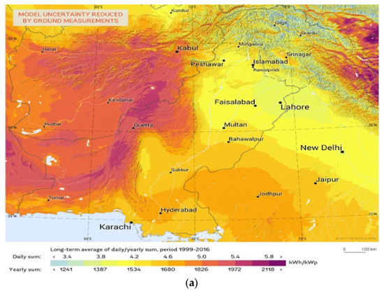
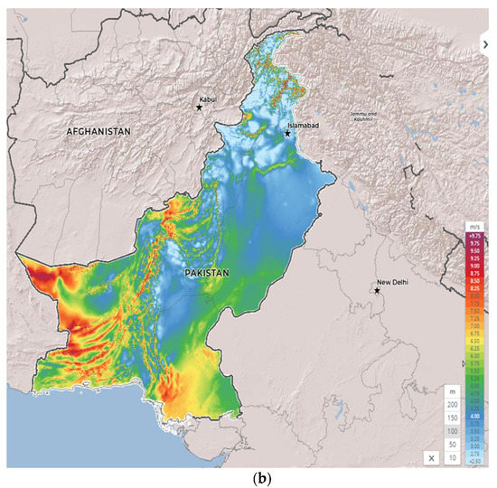
Figure 9.
(a) Solar potential and (b) wind speed map [50,51].
Figure 9.
(a) Solar potential and (b) wind speed map [50,51].
4. Scenario Definition
4.1. Demand Side
Baseline (Reference):
- The future GDP growth rate and inflation are assumed to be 5.5% and 4.1%, respectively. The sectoral share of GVA is assumed to be consistent with the base year for economic sectors.
- The projection of population is referred to as the medium variant of estimation of the United Nations. The share of different fuels in all sectors is assumed to be constant at the base year level.
Economic Growth [EG]:
To assess the impact of economic growth with respect to the baseline scenario, two economic growth scenarios are devised, as follows:
- High Economic Growth (HEG): A growth rate of 7% is assumed to this level of economic activity.
- Low Economic Growth (LEG): In this scenario, a growth rate of 3% is considered. It is lower than the baseline scenario.
4.2. Supply Side
Renewable [REN]:
- According to the Renewable Policy 2019, the system gradually accommodates a 20% share by 2025 and a 30% share by 2030 of solar, wind, and waste- and biobased power plants.
No Coal [NC]:
- In the wake of climate change challenges, referring to a recent statement by the government regarding the commitment to no more installations of new coal-based power plants, the existing planned and under-construction coal-based power plants are considered for the analysis.
5. Results and Discussion
5.1. Demand-Side Analysis
5.1.1. Baseline Scenario
In this study, EViews software was employed to analyze the data sets of each demand sector. The Augmented Dickey–Fuller (ADF) test is used to check the stationarity of the time series data (see Table A1 in Appendix A). The result revealed that none of the variables is stationary at its level (i.e., I(0)). This suggests that multiple regression cannot be applied. This situation leads to the application of the ARDL model. Table 16 summarizes the optimal lag orders of variables in the ARDL model and the performance of the statistical analysis. R2 results are convincing, and the Durbin–Watson test is within limits. The results of the detailed ARDL model are given in Table A2 in Appendix B.

Table 16.
The results for econometric analysis for different sectors.
Table 17 shows the long-term results extracted from the ARDL model. Energy price has an expected negative sign, and consumption/value added has a positive sign. Different sectors exhibit different behavior. The household and transport sectors are less affected by the energy price. This may be a possible consequence of the energy subsidies provided in this sector and low tariffs for domestic natural gas. However, income has a significant positive impact in both sectors.

Table 17.
Results for long-term analysis.
Figure 10a shows the projected sectoral energy demand for the period 2017–2032. Figure 10b provides an outlook on the demand for different fuels within the model horizon. On an aggregative level, the transport sector shows the highest growth of overall energy demand. For the given growth rate of GDP, the ownership of cars, a comparatively high energy-intensive transport mode, is estimated to increase from 39 vehicles/1000 person to 260 vehicles/1000 person. This trend may be referred to as moderate economic growth, increasing transportation demand due to improved incomes and sustaining economic growth. The rising of the total energy demand can result from enhanced lifestyle, urbanization, and economic activities.
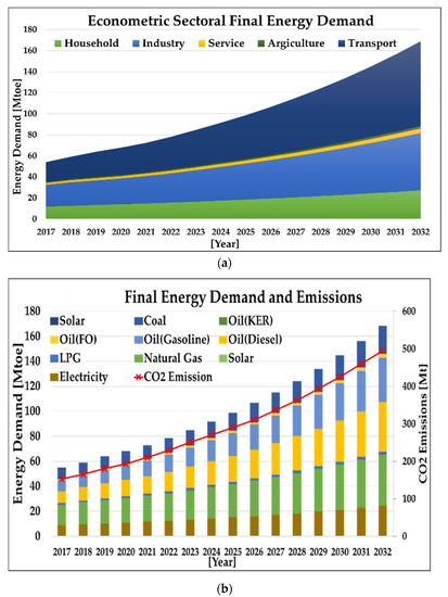
Figure 10.
(a) Results for sectoral energy projections. (b) Disaggregation of demand into fuels.
The electricity demand is expected to increase from its current 8.70 Mtoe [106.7 TWh] to 24.19 Mtoe [297.2 TWh], with an annual average growth rate of 6.60%. The results are comparable to other recent studies. The NTDC [9] projected 303.55 TWh for the year 2032–33, Miraj et al. [13] estimated 330.1 TWh for the year 2030, Gul and Qureshi [19] projected 368 TWh in 2030, and Perwez et al. [53] 312 TWh in 2032.
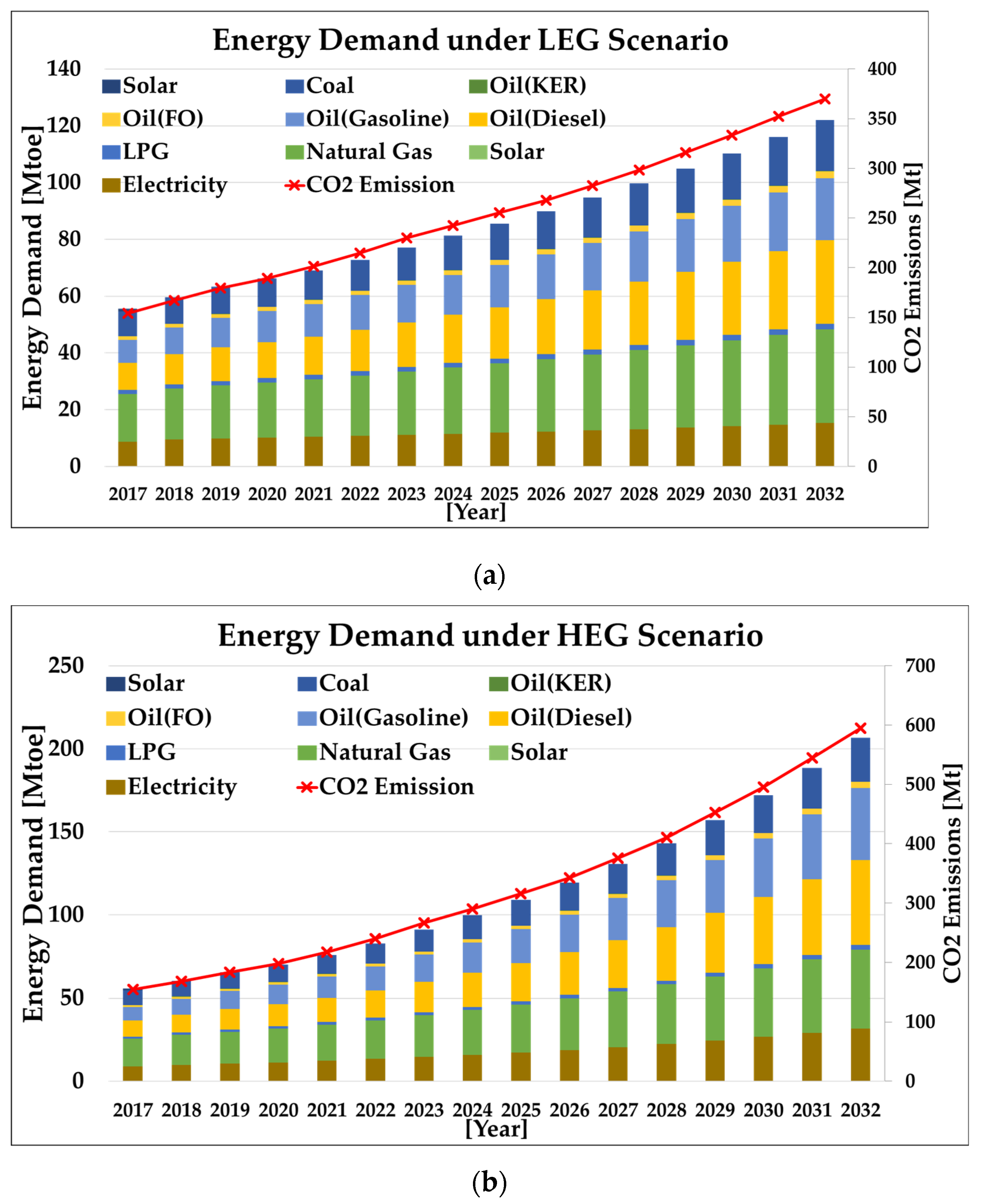
Natural gas demand is expected to grow at an annual average rate of 5.85%. The results of natural gas demand forecasting by the Oil and Gas Regulatory Authority (OGRA) [48] showed a yearly growth rate of 4.13% until 2028, which is lower than this study. The demand for other fuels, i.e., gasoline, HSD, FO, coal, LPG, and kerosene oil, is estimated to grow at 9.55%, 9.30%, 6.26%, 3.68%, and 4.41%, respectively, on an average annual basis. Considering the emission factor for different fuels from IPCC, CO2 emissions are expected to increase from 153 MT to 495 MT with an annual growth rate of 7.60%.
5.1.2. Economic Scenario
Figure 11 shows the results for energy demand for each fuel and resulting emissions. In the LEG case, the overall energy demand and emission are 28.13% and 25.55% lower than the baseline demand. For HEC, the overall energy demand and emission are 21.74% and 19.71% higher than the baseline demand.
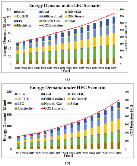
Figure 11.
Energy demand and emission under (a) LEG and (b) HEG scenarios.
5.2. Supply-Side Analysis
5.2.1. Baseline Scenario
Figure 12 shows the optimum selection of power generation technologies for the given baseline scenario demand from the demand model. A significant technological change can be observed during the prediction horizon. HSD- and RLNG (CT)-based power plants are excluded from the power supply mix after the base year due to high fuel cost, and a major contribution is provided by the additional capacity installation of natural gas-based power plants. Natural gas-based power plants also started to retire gradually after 2021 and will phase out by 2024. This corresponds to the depletion of natural gas production after 2021. Imported coal shows a consistent rise from 8.3% in 2017 to 46% in 2032. Local coal contribution increases to 22.6% in the energy supply mix from 2020 to 2032. Nuclear power plants show relatively slow progress from 7.5% to 14.2% within the model horizon. RLNG-based combined-cycle power plants operate until 2022, after which they lose their economic competitiveness to local and imported coal. On the renewable side, the share of hydropower is reduced from 21.2% [2017] to 13.9% [2032]. Other than the planned deployment, the rest of the renewables are selected for new installation, and hence their share in power generation is declined over time. Coal (local and imported) power plants are the main consideration for new capacity installations. The emissions from the generation side are increased from 55 MT to 182.3 MT. The increasing share of coal-based power generation is the main reason for such a rapid rise in emissions. The overall levelized cost of energy (LCOE) is computed to be 7.00 Cents/kWh. The model was given the option to include storage as needed, but the flexibility provided by the other sources (mainly hydro) was sufficient to accommodate RE share, even in the subsequent scenarios involving high RE penetration.
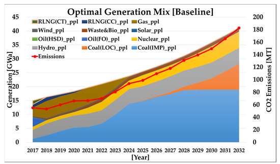
Figure 12.
Optimal generation mix along with resulting emissions for the baseline scenario.
5.2.2. REN and NC Scenario
Figure 13 shows the comparison of the renewable and no coal scenario with the baseline case. In the NC scenario, restrictions on the future installation of coal-based power plants will force the model toward significant investment in hydropower during the period of 2023–2024, solar and wind, respectively, in subsequent years, leading to a share of 62.61% in 2032. In the REN scenario, the enhanced share of solar, wind, and waste and bio offset the installation of coal-based power plants. The rest of the power plants do not have any impact on their investment decisions. In terms of LCOE and emission reduction potential, NC is an expensive scenario with 8.00 cents/kWh but has more potential for emission reduction. For the REN scenario, the emissions are 24.48% lower than the baseline case. Table 18 shows the summary of emission reductions, cost, and renewable shares in the different scenarios.
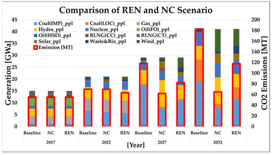
Figure 13.
The comparison of REN and NC Scenarios with the baseline.

Table 18.
Summary of analysis of different scenarios on the supply side.
5.3. Emission Reduction Targets
Setting emission reduction targets will result in a sharp rise in renewable penetration and phasing out of coal-based power plants. Table 19 summarizes the impact of different emission-bound targets on the cost and generation mix.

Table 19.
Sensitivity analysis of emission reduction targets.
In the strictest target (50% annual emission reduction), the renewable share is estimated to reach 82.74%, compared to 17.16% in the baseline. The contribution of imported coal in total power generation will be reduced to zero in 2032. However, local coal has a small share due to cost consideration, as shown in Figure 14. Hydropower replaces natural gas-based power plants in 2024. In 2032, hydro and wind together account for 66% of total power generation. Hence, the LCOE is 21% higher than the baseline due to investment in comparatively expensive options.
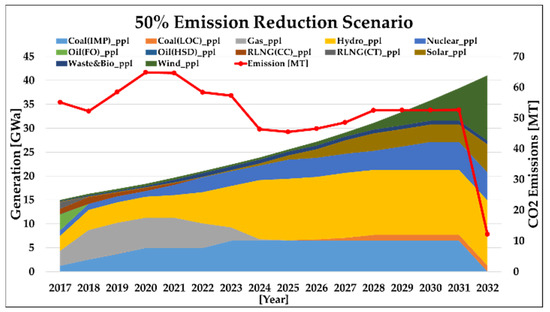
Figure 14.
Generation mix and resulting CO2 emissions for 50% reduction in emission scenario.
5.4. Integrated Demand-Supply Scenarios Analysis
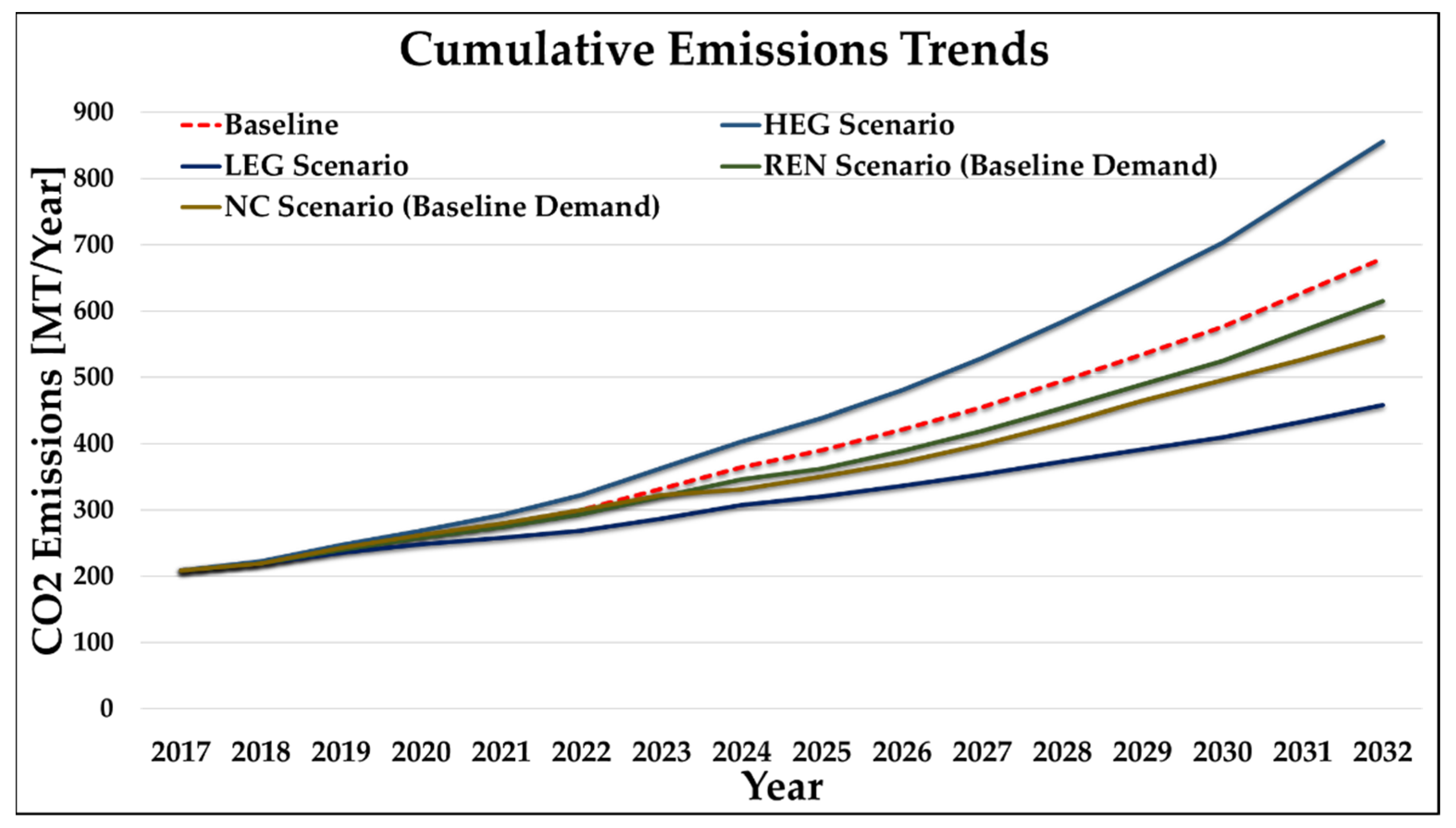
Integrated energy modeling, used in this study, combines the effect of macrolevel demand analysis with its bottom-up supply dynamics, considering the technological details and constraints. Such a modeling approach may be helpful to assess the overall outlook of energy systems under a wide range of policies, targets, and constraints on either the demand or supply side. The proposed approach should not be perceived as an alternative, but rather as an intermediary step to more traditional and comprehensive energy-related models. This model analysis, which is dynamic and consisting of three phases (top-down and bottom-up on the demand side and bottom-up on the supply side), can be applied for assessing the consistency of future scenarios and policy requirements to reduce energy intensity while simultaneously promoting the cost-efficient use of sustainable (i.e., renewable) energy sources in Pakistan. The implications of this type of analysis may involve the evaluation of various energy sector-related frameworks planned in the National Climate Change Policy introduced by the Government of Pakistan in 2012 aimed at curbing climate change impacts. Figure 15 presents the cumulative (demand- and supply-side combined) emissions trends under different scenarios. For supply-side scenarios, the baseline demand is considered. In demand-side scenarios, the emissions contribution from the supply side is more significant than the demand side. For example, in high economic growth (HEG), the cumulative emissions are increased at an annual average of 14.94%, whereas the demand and supply side show an increased rate of 10.51% and 27.76%, respectively. This quantification and evaluation can cover other areas, such as resource explorations, regional energy trade, improvement in energy efficiency, rural electrification, structural reforms, and electrification of traditional fossil fuel-based applications in the household and transport sectors.
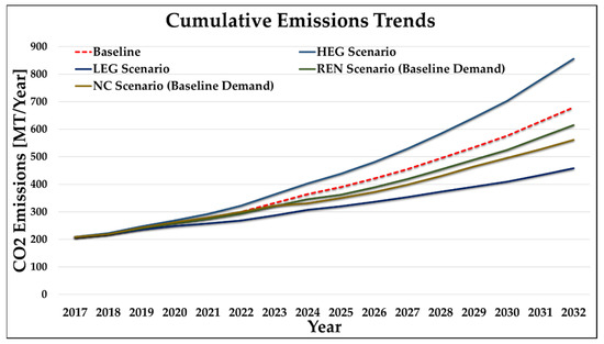
Figure 15.
Cumulative emissions trends under different scenarios.
6. Challenges and Opportunities
Pakistan is an underdeveloped country; its government is always striving to intervene through various policies on the economic front to raise the level of economic activity and consequently the wellbeing of the public. Based on the analysis of energy demand in this study, energy demand is a key driver of economic growth, both on the production and consumption sides, and thus has significant economic, social, and environmental impacts following the baseline trend. The analysis and projection of future demand under different scenarios conducted in this study may help the government to be well prepared to intervene in advance with policy measures to foresee growing demand and counter its resulting environmental impacts under different levels of economic activity growth. The improved economic situation may help offset reasonable investments made on the demand side to reduce carbon footprints, such as improvement in energy efficiency. The sectoral analysis of demand can help estimate the overall demand impact of emphasizing specifically, i.e., the low energy-intensive sector. For the same level of economic activity, the energy demand drastically differs as the economic structure changes.
On the supply side, policy interventions based on the Renewable Policy 2019 by the Alternate Energy Development Board (REN Scenario) and restrictions on future coal-based power generation (NC Scenario) suggest the NC scenario as a more practical option in reducing emissions, although it has its economic implications. The coal phase-out will be compensated by high-capacity investments in renewables (hydro, wind, and solar) and raising the level of domestic energy reliance. For example, under this scenario, the capacity of the hydro power plant is estimated to reach a level of 23.22 GW in 2032, including a large additional capacity of 7.54 GW in 2024. The high-capacity investment in hydropower can assist the power system with absorbing more of the other less flexible renewable sources. Solar and wind power will require a total installed capacity of 19.69 GW and 29.97 GW in 2032.
On the other hand, the nuclear power contribution is not quite significant compared to the baseline scenario. These are critical policy decisions that the government must consider while pursuing such ambitious environmental protection and energy security enhancement targets. In the short run, if the policy decisions are made to invest more in RLNG-based power plants, with less environmental impact than coal-based plants, to react to coal restrictions, it will cause an increased burden on foreign exchange, circular debt, and the cost of electricity. These are the different trade-offs that the government needs to consider to realize a better energy system and management of resources.
Until 2032, a renewable share of 20% by 2025 and 30% by 2030 (REN Scenario) will replace coal-based (local and imported) generation. The rest of the options do not contribute to this change significantly. However, due to the reliability limitation of high renewable penetration, the overall required system capacity in 2032 will be 77.45 GW, which is 47% more than the baseline scenario. This is one of the main challenges to deploying renewable for the same amount of electricity generation, such that the demand for capacity and storage become significant. To avoid the curtailment of renewable energy, special analysis of the correlation of renewable generation with the electricity demand profile and the design of special demand response programs must help to prepare an operational/dispatch plan. For this model horizon, the existing generation options are sufficient to provide the flexibility demanded by the renewable sources. However, as we head into the future with similar targets of renewable energy, this flexibility requirement will become very critical and may require the exploration of different kinds of storage options or investment in conventional flexible options, such as RLNG-based power plants.
7. Conclusions
This study aimed to introduce a comprehensive and integrated energy model for Pakistan to project energy demand and optimize the supply mix under different scenario options. The research emphasized developing an integrated energy modeling framework in order to have a comprehensive analysis of the energy sector in Pakistan, which may lead to effective policy and decision-making. Reliable forecasting of economic parameters in the short and long term can help obtain better energy demand projections. Through an analysis of energy supply and demand and carbon emission data for the scenarios, it is obvious that energy demand will continue to grow up to 2030, resulting from enhanced lifestyles, urbanization, and economic activities in Pakistan. According to the results, in the baseline case, the energy demand is estimated to increase from 8.70 Mtoe [106.7 TWh] to 24.19 Mtoe [297.2 TWh], with an annual average growth rate of 6.60%. The total energy demand and emission are estimated to be 21.74% and 19.71% higher in the HEG scenario and, on the other hand, 28.13% and 25.55% lower in the LEG scenario, compared to the baseline scenario. On the supply side, coal-based power generation is the most economical option but has the worst environmental impact. The depletion of domestic natural gas production will result in a substantial change on the power generation side. A policy to ban the installation of new coal-based power plants (i.e., NC scenario) reduces average emissions by 37.4%, which requires an increase in the share of renewable energy in power generation up to 62%. In the REN scenario, increasing the share of renewable energy power generation by 2030 can help to reduce emissions by 24%, which is accompanied by a 13% increase in the total cost of power generation. The results of this study indicate that the REN and NC scenarios meet most of Pakistan’s economic and environmental requirements. Following the proposed scenarios, Pakistan’s energy supply system could be independent of imports, thus reducing both costs and pollution. However, strict environmental regulation will demand renewable energy penetration and investment in the power sector. Decarbonization is the basic characteristic of the structural changes to energy supply and demand in Pakistan. Renewable energies will replace coal as the largest energy source prior to 2030 in a 50% reduction scenario. In the context of environmental protection, the significant achievements of low-pollution strategies in Pakistan’s energy system can be obtained through concurrent improvements on both the supply and demand sides. In this context, the application of energy systems modeling with further policy formulation would be needed to test various hypotheses and policy perspectives. Future research will involve the following areas.
- Expending the model horizon to accommodate advanced and prospect carbon mitigation technologies (i.e., carbon capture and utilization, coal liquefaction);
- Evaluation of capacity value or contribution (based on the correlation of generation with load profile) for renewable sources;
- Enhancement of temporal resolution to include more details on operation and load patterns (i.e., seasonality);
- Analysis of conventional schemes, various storage options, and demand response programs to match the flexibility requirements in high penetration of renewable energy sources in the future;
- Updating the estimation of the trend of extraction of local resources;
- Estimating the future costs of local resources and imported energy commodities, especially the analysis of imported LNG in case of the depletion of domestic natural gas reserves;
- Study of more scenarios on the demand and supply sides, such as the impact of fuel switching (from traditional biomass to modern and clean options) in the residential sector.
Author Contributions
Conceptualization and methodology: S.A. and H.F.; Investigation: S.A.; Writing: S.A. and H.F.; Review, editing: H.F.; Supervising: H.F. All authors have read and agreed to the published version of the manuscript.
Funding
This research was supported by the Japanese Grant Aid for Human Resource Development (JDS).
Institutional Review Board Statement
Not applicable.
Informed Consent Statement
Not applicable.
Data Availability Statement
Not applicable.
Conflicts of Interest
The authors declare no conflict of interest.
Appendix A

Table A1.
Results for Augmented Dickey–Fuller test to check stationarity.
Table A1.
Results for Augmented Dickey–Fuller test to check stationarity.
| Sectors | Variable | Level | First Diff. | Decision | ||
|---|---|---|---|---|---|---|
| t-Stat | p-Val. | t-Stat | p-Val. | |||
| Household (HH) | ln (EC_HH)t | −0.589 | 0.853 | −6.556 | 0.000 | I(1) |
| ln (EP_HH)t | −2.469 | 0.137 | −5.040 | 0.001 | I(1) | |
| ln (CONS)t | 0.794 | 0.991 | −3.887 | 0.009 | I(1) | |
| Transport (TRNS) | ln (EC_TRNS)t | 1.065 | 0.996 | −4.050 | 0.006 | I(1) |
| ln (EP_TRNS)t | −1.625 | 0.453 | −3.837 | 0.009 | I(1) | |
| ln (CONS)t | 0.794 | 0.991 | −3.887 | 0.009 | I(1) | |
| Industry (IND) | ln (EC_IND)t | −0.840 | 0.785 | −2.475 | 0.136 | I(2) |
| ln (EP_IND)t | −1.60758 | 0.461 | −6.5936 | 0.000 | I(1) | |
| ln (VA_IND)t | −0.47101 | 0.879 | −4.20294 | 0.0043 | I(1) | |
| Service (SRV) | ln (EC_SRV)t | −1.05949 | 0.71 | −2.64199 | 0.1015 | I(2) |
| ln (EP_SRV)t | −2.31065 | 0.178 | −5.88428 | 0.0001 | I(1) | |
| ln (VA_SRV)t | 0.094845 | 0.957 | −2.33057 | 0.1727 | I(2) | |
| Agriculture (AGRI) | ln (EC_AGRI)t | −2.24377 | 0.198 | −3.29012 | 0.0293 | I(1) |
| ln (EP_AGRI)t | −1.77701 | 0.38 | −2.90758 | 0.0621 | I(2) | |
| ln (VA_AGRI)t | −0.77251 | 0.806 | −6.0167 | 0.0001 | I(1) | |
Note: The critical values of the ADF test were referred to [54].
Appendix B

Table A2.
Short-term results for econometric analysis of demand.
Table A2.
Short-term results for econometric analysis of demand.
| Sector | Variable | Coefficient | Std. Error | t-Stat | Prob. |
|---|---|---|---|---|---|
| Household (HH) | ln(EC_HH)t−1 | 0.402 | 0.179 | 2.249 | 0.038 |
| ln(EP_HH)t | −0.046 | 0.057 | −0.814 | 0.427 | |
| ln(CONS)t | 0.622 | 0.189 | 3.289 | 0.004 | |
| Constant | −8.568 | 2.680 | −3.196 | 0.005 | |
| Transport (TRNS) | ln(EC_TRNS)t−1 | 0.652 | 0.254 | 2.568 | 0.030 |
| ln(EC_TRNS)t−2 | −0.554 | 0.271 | −2.046 | 0.071 | |
| ln(EC_TRNS)t−3 | 0.202 | 0.229 | 0.879 | 0.402 | |
| ln(EP_TRNS) | −0.289 | 0.071 | −4.080 | 0.003 | |
| ln(EP_TRNS)t−1 | 0.255 | 0.129 | 1.976 | 0.080 | |
| ln(EP_TRNS)t−2 | −0.265 | 0.120 | −2.213 | 0.054 | |
| ln(CONS)t | 0.616 | 0.382 | 1.611 | 0.142 | |
| ln(CONS)t−1 | −0.776 | 0.568 | −1.365 | 0.205 | |
| ln(CONS)t−2 | 1.055 | 0.448 | 2.357 | 0.043 | |
| Constant | −13.009 | 3.605 | −3.608 | 0.006 | |
| Industry (IND) | ln(EC_IND)t−1 | 0.876 | 0.248 | 3.533 | 0.003 |
| ln(EC_IND)t−2 | −0.406 | 0.193 | −2.109 | 0.052 | |
| ln(EP_IND)t | −0.283 | 0.116 | −2.434 | 0.028 | |
| ln(VA_IND)t | 0.402 | 0.152 | 2.654 | 0.018 | |
| Constant | −0.911 | 2.196 | −0.415 | 0.684 | |
| Service (SRV) | ln(EC_SRV)t−1 | 0.677 | 0.175 | 3.864 | 0.001 |
| ln(EP_SRV)t | −0.108 | 0.075 | −1.434 | 0.171 | |
| ln(VA_SRV)t | 1.191 | 0.558 | 2.136 | 0.049 | |
| ln(VA_SRV)t−1 | −0.853 | 0.594 | −1.435 | 0.171 | |
| Constant | −4.559 | 3.360 | −1.357 | 0.194 | |
| Agriculture (AGRI) | ln(EC_AGRI)t−1 | 0.289 | 0.212 | 1.362 | 0.206 |
| ln(EC_AGRI)t−2 | 0.400 | 0.220 | 1.815 | 0.103 | |
| ln(EC_AGRI)t−3 | −0.750 | 0.178 | −4.199 | 0.002 | |
| ln(EP_AGRI)t | −0.578 | 0.133 | −4.329 | 0.002 | |
| ln(EP_AGRI)t−1 | 0.288 | 0.158 | 1.824 | 0.102 | |
| ln(EP_AGRI)t−2 | 0.057 | 0.136 | 0.416 | 0.687 | |
| ln(EP_AGRI)t−3 | −0.309 | 0.162 | −1.905 | 0.089 | |
| ln(VA_AGRI)t | −0.507 | 0.571 | −0.888 | 0.397 | |
| ln(VA_AGRI)t−1 | 1.152 | 0.617 | 1.866 | 0.095 | |
| Constant | −0.077 | 3.773 | −0.020 | 0.984 |
References
- UN. Paris Agreement; UN: New York, NY, USA, 2015. [Google Scholar]
- Farzaneh, H. Devising a Clean Energy Strategy for Asian Citie; Springer Nature: Basingstoke, UK, 2019. [Google Scholar]
- GERMANWATCH. Global Climate Risk Index 2020; GERMANWATCH: Bonn, Germany, 2020. [Google Scholar]
- UNFCCC. Pakistan’s Intended Nationally Determined Constribution (PAK-INDC); UNFCCC: Bonn, Germany, 2016. [Google Scholar]
- International Energy Agency. CO2 emissions from fuel combustion. Outlook 2019, 1–92. [Google Scholar]
- Perwez, U.; Sohail, A. Forecasting of Pakistan’s net electricity energy consumption on the basis of energy pathway scenarios. Energy Procedia 2014, 61, 2403–2411. [Google Scholar] [CrossRef]
- Farooq, M.K.; Kumar, S.; Shrestha, R.M. Energy, environmental and economic effects of renewable portfolio standards (RPS) in a developing country. Energy Policy 2013, 62, 989–1001. [Google Scholar]
- Arif, A.; Rizwan, M.; Elkamel, A.; Hakeem, L.; Zaman, M. Optimal selection of integrated electricity generation systems for the power sector with low greenhouse gas (GHG) emissions. Energies 2020, 13, 4571. [Google Scholar] [CrossRef]
- NTDC. IGCEP Plan 2018–2040; NTDC: Lahore, Pakistan, 2019.
- Ur Rehman, S.A.; Cai, Y.; Fazal, R.; Walasai, G.D.; Mirjat, N.H. An integrated modeling approach for forecasting long-term energy demand in Pakistan. Energies 2017, 10, 1868. [Google Scholar]
- Ur Rehman, S.A.; Cai, Y.; Siyal, Z.A.; Mirjat, N.H.; Fazal, R.; Kashif, S.U.R. Cleaner and sustainable energy production in Pakistan: Lessons learnt from the Pak-times model. Energies 2019, 13, 108. [Google Scholar] [CrossRef]
- Jamil, R. Hydroelectricity consumption forecast for Pakistan using ARIMA modeling and supply-demand analysis for the year 2030. Renew. Energy 2020, 154, 1–10. [Google Scholar] [CrossRef]
- Mirjat, N.H.; Uqaili, M.A.; Harijan, K.; Walasai, G.D.; Mondal, M.A.H.; Sahin, H. Long-term electricity demand forecast and supply side scenarios for Pakistan (2015–2050): A LEAP model application for policy analysis. Energy 2018, 165, 512–526. [Google Scholar] [CrossRef]
- Aized, T.; Shahid, M.; Bhatti, A.A.; Saleem, M.; Anandarajah, G. Energy security and renewable energy policy analysis of Pakistan. Renew. Sustain. Energy Rev. 2018, 84, 155–169. [Google Scholar]
- Ishaque, H. Is it wise to compromise renewable energy future for the sake of expediency? An analysis of Pakistan’s long-term electricity generation pathways. Energy Strateg. Rev. 2017, 17, 6–18. [Google Scholar]
- Azam, A.; Rafiq, M.; Shafique, M.; Ateeq, M.; Yuan, J. Causality relationship between electricity supply and economic growth: Evidence from Pakistan. Energies 2020, 13, 837. [Google Scholar] [CrossRef]
- JICA. Project for Least Cost Power Generation and Transmission Expansion Plan Final Report; JICA: Tokyo, Japan, 2016.
- Anwar, J. Analysis of energy security, environmental emission and fuel import costs under energy import reduction targets: A case of Pakistan. Renew. Sustain. Energy Rev. 2016, 65, 1065–1078. [Google Scholar] [CrossRef]
- Gul, M.; Qureshi, W.A. Modeling diversified electricity generation scenarios for Pakistan. In Proceedings of the 2012 IEEE Power and Energy Society General Meeting, San Diego, CA, USA, 22–26 July 2012; pp. 1–7. [Google Scholar]
- Hussain, A.; Rahman, M.; Memon, J.A. Forecasting electricity consumption in Pakistan: The way forward. Energy Policy 2016, 90, 73–80. [Google Scholar] [CrossRef]
- NTDC. Electricity Demand Forecast Based on Multiple Regression Analysis 2014; NTDC: Lahore, Pakistan, 2014; pp. 1–111.
- Shahbaz, M.; Lean, H.H. The dynamics of electricity consumption and economic growth: A revisit study of their causality in Pakistan. Energy 2012, 39, 146–153. [Google Scholar] [CrossRef]
- Zaman, K.; Khan, M.M.; Ahmad, M.; Rustam, R. Determinants of electricity consumption function in Pakistan: Old wine in a new bottle. Energy Policy 2012, 50, 623–634. [Google Scholar] [CrossRef]
- Farzaneh, H.; Doll, C.N.H.; Puppim De Oliveira, J.A. An integrated supply-demand model for the optimization of energy flow in the urban system. J. Clean. Prod. 2016, 114, 269–285. [Google Scholar] [CrossRef]
- Haider, A.; Husnain, M.I.U.; Rankaduwa, W.; Shaheen, F. Nexus between nitrous oxide emissions and agricultural land use in agrarian economy: An ardl bounds testing approach. Sustainability 2021, 13, 2808. [Google Scholar] [CrossRef]
- Abumunshar, M.; Aga, M.; Samour, A. Oil price, energy consumption, and CO2 emissions in Turkey. New evidence from a bootstrap ARDL test. Energies 2020, 13, 5588. [Google Scholar] [CrossRef]
- Busu, M. Analyzing the impact of the renewable energy sources on economic growth at the EU level using an ARDL model. Mathematics 2020, 8, 1367. [Google Scholar] [CrossRef]
- Samuelson. Foundations of Economic Analysis, Enlarged Edition; Harvard University Press: Cambridge, MA, USA, 1983. [Google Scholar]
- Farzaneh, H. Energy Systems Modeling: Principles and Applications; Springer: New York, NY, USA, 2019. [Google Scholar]
- Huppmann, D.; Gidden, M.; Fricko, O.; Kolp, P.; Orthofer, C.; Pimmer, M.; Kushin, N.; Vinca, A.; Mastrucci, A.; Riahi, K.; et al. The MESSAGEix Integrated Assessment Model and the ix modeling platform (ixmp): An open framework for integrated and cross-cutting analysis of energy, climate, the environment, and sustainable development. Environ. Model. Softw. 2019, 112, 143–156. [Google Scholar] [CrossRef]
- Sullivan, P.; Krey, V.; Riahi, K. Impacts of considering electric sector variability and reliability in the MESSAGE model. Energy Strateg. Rev. 2013, 1, 157–163. [Google Scholar] [CrossRef]
- Ministry of Energy (Petroleum Division) Hydrocarbon Development Institute of Pakistan. Pakistan Energy Year Book 2018. 2018; 156. [Google Scholar]
- World Bank. World Development Indicators (WDI); World Bank: Washington, DC, USA, 2021. [Google Scholar]
- Pakistan Burea of Statistics. Pakistan Social and Living Standards Measurement Survey; Pakistan Burea of Statistics: Islamabad Pakistan, 2015.
- Pakistan Bureau of Statistics. District Wise Population by Sex and Rural/Urban Government of Pakistan. 6th Population Census; Pakistan Bureau of Statistics: Islamabad, Pakistan, 2017; Volume 13.
- United Nations, Department of Economic and Social Affairs, Population Division (2019). World Population Prospects 2019, Online Edition. Rev. 1. Available online: https://population.un.org/wpp/ (accessed on 1 May 2021).
- Finance Division (Government of Pakistan). Economic Survey (Multiple Issues) 2017-18. 2018. Available online: http://www.finance.gov.pk/survey_1718.html (accessed on 1 May 2021).
- PEC. Buidling Codes of Pakistan (Energy Provision 2011); Pakistan Engineering Council: Islamabad, Pakistan, 2011. [Google Scholar]
- Amber, K.P.; Aslam, M.W.; Ikram, F.; Kousar, A.; Ali, H.M.; Akram, N.; Afzal, K.; Mushtaq, H. Heating and cooling degree-days maps of Pakistan. Energies 2018, 11, 94. [Google Scholar] [CrossRef]
- Biresselioglu, M.E.; Demir, M.H.; Rashid, A.; Solak, B.; Ozyorulmaz, E. What are the preferences of household energy use in Pakistan?: Findings from a national survey. Energy Build 2019, 205, 109538. [Google Scholar] [CrossRef]
- Ravindranath, N.H.; Ramakrishna, J. Energy options for cooking in India. Energy Policy 1997, 25, 63–75. [Google Scholar] [CrossRef]
- Sudhakara Reddy, B. Electrical vs solar water heater: A case study. Energy Convers. Manag. 1995, 36, 1097–1106. [Google Scholar] [CrossRef]
- Shabbir, R.; Ahmad, S.S. Monitoring urban transport air pollution and energy demand in Rawalpindi and Islamabad using leap model. Energy 2010, 35, 2323–2332. [Google Scholar] [CrossRef]
- Saxena, S.; Gopal, A.; Phadke, A. Electrical consumption of two-, three- and four-wheel light-duty electric vehicles in India. Appl. Energy 2014, 115, 582–590. [Google Scholar] [CrossRef]
- The National Renewable Energy Laboratory (NREL). Annual Technology Baseline (ATB) 2019. Available online: https://atb.nrel.gov/electricity/2019/summary.html (accessed on 1 May 2021).
- Ghafoor, A.; Rehman, T.U.; Munir, A.; Ahmad, M.; Iqbal, M. Current status and overview of renewable energy potential in Pakistan for continuous energy sustainability. Renew. Sustain. Energy Rev. 2016, 60, 1332–1342. [Google Scholar] [CrossRef]
- Private Power and Infrastructure Board. Pakistan Hydel Power Potential. Pakistan Hydel. Power Potential, 2002; 112. [Google Scholar]
- Oil & Gas Regulatory Authority of Pakistan. State of regulated petroleum industry 2017–2018. 2019; 53, 1689–1699. [Google Scholar]
- Ministry of Planning, Development and Reforms (Government of Pakistan). Pakistan 2025. Available online: https://www.pc.gov.pk/uploads/vision2025/Pakistan-Vision-2025.pdf (accessed on 1 May 2021).
- Global Solar Atlas 2.0, Web-Based Application Is Developed and Operated by the Company Solargis s.r.o. on Behalf of the World Bank Group, Utilizing Solargis Data, with Funding Provided by the Energy Sector Management Assistance Program (ESMAP). Available online: https://globalsolaratlas.info (accessed on 1 May 2021).
- Global Wind Atlas 3.0, a Free, Web-Based Application Developed, Owned and Operated by the Technical University of Denmark (DTU). The Global Wind Atlas 3.0 is Released in Partnership with the World Bank Group, Utilizing Data Provided by Vortex, Using Funding Provided by the Energy Sector Management Assistance Program (ESMAP). Available online: https://globalwindatlas.info (accessed on 1 May 2021).
- Savin, N.E.; White, K.J. The Durbin-Watson Test for Serial Correlation with Extreme Sample Sizes or Many Regressors. Econometrica 1977, 45, 1989–1996. [Google Scholar] [CrossRef]
- Perwez, U.; Sohail, A.; Hassan, S.F.; Zia, U. The long-term forecast of Pakistan’s electricity supply and demand: An application of long range energy alternatives planning. Energy 2015, 93, 2423–2435. [Google Scholar] [CrossRef]
- Mackinnon, J.G. Numerical distribution functions for unit root and cointegration tests. J. Appl. Econom. 1996, 11, 601–618. [Google Scholar] [CrossRef]
Publisher’s Note: MDPI stays neutral with regard to jurisdictional claims in published maps and institutional affiliations. |
© 2021 by the authors. Licensee MDPI, Basel, Switzerland. This article is an open access article distributed under the terms and conditions of the Creative Commons Attribution (CC BY) license (https://creativecommons.org/licenses/by/4.0/).

