Development and Validation of a Dynamic Simulation Model for an Integrated Solar Combined Cycle Power Plant

Abstract

The combined cycle power plants are the most recognized thermal power plants for their high efficiency, fast start-up capability, and relatively low environmental impact. Moreover, their flexible unit dispatch supports the share of renewable energy, which contributes to carbon mitigation. The operational flexibility of Integrated Solar Combined Cycle (ISCC) power plants is a crucial factor for reliable grid stability. To evaluate the limitations and capabilities of ISCC power plants and their control structures, dynamic simulation is a feasible method. In this study, a sophisticated dynamic process model of the ISCC power plant in Kuraymat, Egypt, has been developed using APROS software. The model describes the plant with a high level of detail including the solar field, the heat recovery steam generator, and the control structures. The model was implemented structurally identical to the reference plant and tuned using the operational design data. Actual measurements were used as the basis for the initialization and validation of the dynamic simulation environment. Dynamic analysis of four different days was performed, then the simulation results were presented and compared with actual measurements. The comparison showed that the course of the actual measurements could be predicted with high accuracy. The solar field influences and the system’s overall power curves are reliably simulated. Consequently, the validated model can simulate the dynamic behavior of the ISCC power plant with a high degree of accuracy, and can be considered in future planning decisions.

1. Introduction

Electricity demand is growing worldwide faster than any other form of energy consumption as a result of increasing population growth, digitalization, e-mobility and sector coupling. The share of electricity produced from thermal power plants continues to dominate total electricity production worldwide, and thermal power plants share more than 80% of electricity production worldwide and are set to remain a major player for the foreseeable future [1]. Thermal power generation includes electricity produced from coal (38.2%), natural gas (23.1%), nuclear (10.2%), petroleum (2.9%), and non-renewables and waste (9.8%) [1]. Retrofitting thermal power plants for flexible operation can contribute to the integration of renewable energies into a modern power supply system. The combined cycle power plants (CCPP) are the most recognized thermal power plants for their high efficiency, fast start-up capability, and relatively low environmental impact. Besides, their flexible unit dispatch supports the increase in the share of renewable feed-in.

Energy from renewables is expected to make a significant contribution to the carbon mitigation required for achieving the European and global climate change mitigation goal of keeping the maximum average global temperature rise below 1.5 °C [2]. The European Union and their member states intend to promote the expansion of renewable energy sources of at least 32% of the gross final energy consumption by 2030 because energy from renewables will play a key role for the years after 2020. However, renewable energy technologies need to be less expensive to be competitive with other power generation technologies. Concentrated Solar Power (CSP) technology is one of the renewable energy technologies that uses mirrors or lenses, or a combination of both, to concentrate the sun’s rays and convert their energy into very high-temperature heat to produce steam to drive steam turbines that generate electricity. CSP technologies such as parabolic trough collectors can be coupled with heat storage technologies to produce electricity on demand regardless of irradiation conditions, but heat storage technologies are not yet affordable. The integration of CSP technology with CCPP contributes to reducing the electricity generation costs from solar energy technologies by using the already existing components such as the steam turbine, generator, pumps and condenser. The Integrated Solar Combined Cycle (ISCC) power plants were initially proposed by Luz Solar International after studying them since the 1990s [3]. From 1990 to 2000, the building of new parabolic trough power plants has stopped due to different economic reasons. In 2000, the Global Environment Facility decided to grant up to $50 million for the construction of four ISCC power plants in some developing countries with high solar irradiation, most of them located in the Middle East region. This decision increased interest in CSP technologies again, especially in parabolic trough collectors [4]. The ISCC power plants could play a role as a major contribution to meeting energy demand safely and reliably. The integration of solar-driven technologies into conventional power plants have challenges in the design and optimization of retrofitting solar thermal power plants. The solar integration technology helps to adapt and retrofit the existing power plants instead of developing new ones. The integration of a solar field with a CCPP assures the delivery of the required electricity to the grid regardless of solar radiation conditions, unlike the stand-alone solar power plants.

Mathematical modeling complements the measurement work to better comprehend the principle, performance, and limitations of the energy systems, and contributes to improving its efficiency. The mathematical modeling can be categorized as steady-state simulation and dynamic simulation. The steady-state simulation usually used in the design and optimization of energy systems is based on the mass, momentum, and energy conservation equations in addition to empirical correlations for heat transfer and friction in so-called thermal-hydraulic models. However, the steady-state simulation is only performed for a series of steady-state points and does not provide any information during the transients, and the path between the steady-states may lead to a plant trip. Thus, a relevant next step is to analyze the process using dynamic simulation during transients, load changes, and malfunctions. Unlike the steady-state simulation, the dynamic simulation considers the time derivatives. It is a useful tool throughout the entire service life of a power plant, from proposal to decommissioning. It is a robust and cost-efficient tool for prior assessment of radical operability and controllability of a power plant via design and testing of control structures, operating procedures, and protective and relief devices. In contrast to steady-state process simulation, dynamic process simulation enables detailed acquisition of plant behavior during transients (e.g., load changes, disturbances, start-up and shutdown phases, etc.) with the associated control systems. Dynamic simulation is a feasible way to evaluate the limitations and capabilities of the power plants and their control structures [5]. This requires the accuracy of the model in representing the power plant and the efficiency of the simulation software. The accurate characterization of the system components and automation structures are essential for obtaining a meaningful dynamic response. The requirements for an accurate model are extremely complex. In order to be able to achieve the highest possible degree of accuracy, not only must the individual subsystems be optimally physically coordinated, but the behavior of components, material properties and control mechanisms must also be precisely coordinated.

In the literature, the dynamic process simulation of ISCC power plants is less presented than the steady-state process simulation. The dynamic simulation validation is a key aspect to evaluate these ISCC power plants realistically and reliably to make a well-founded decision on their technological feasibility. In particular, a few studies that have addressed the dynamic simulation complemented their models with actual measurement validation.

J. Spelling et al. [6] performed a thermo-economic optimization of a CCPP integrated with a solar tower with a developed dynamic model using the in-house simulation tool SOLARDYN. This dynamic model is used to obtain the minimal initial investment cost as well as the minimal level of electricity cost. They concluded that the ISCC power plants are both economical and thermodynamically promising after they are properly designed, and they have a competitive level of electricity cost compared with those of other solar thermal power plants.

G. Franchini [7] dynamically simulated a solar Rankine cycle and an ISCC by adopting the TRNSYS types of the solar thermal electric components library. The simulation results revealed that the ISCC has a higher solar-to-electric efficiency than the solar Rankine cycle, and using the solar tower technology assured a higher annual solar-to-electric efficiency, about 21.8%, compared to parabolic trough collectors.

C. Ponce et al. [8] designed a dynamic simulator for an ISCC power plant using MATLAB Simulink^®, based on a solar power plant simulator and a CCPP simulator developed by E. Camacho et al. [9] and D. Sáez et al. [10], respectively. They combined their dynamic simulator with a supervisory control strategy regulating the steam pressure of the superheater (SH) to account for the fuel savings that could be achieved when integrating solar collectors with a CCPP.

F. Calise et al. [11] developed a dynamic simulation model of an ISCC power plant with thermal storage using TRNSYS and presented a thermo-economic and environmental comparison between an ISCC and a conventional combined cycle based on dynamic simulations. The dynamic model verified that the overall electrical efficiency of the ISCC increases, by about 1%, compared to a conventional combined cycle.

B. El Hefni [12] assessed the benefits of converting an existing CCPP to an ISCC power plant regarding the dynamic behavior of the power plant through creating a dynamic model of an ISCC power plant using Modelica. The model was used to simulate the start-up and shutdown of the solar field and to assess its impact on the dynamic behavior of the ISCC power plant.

K. Rashid et al. [13] evaluated the techno-economic performance and the life cycle of a plant-level hybridization (ISCC power plant), compared with grid-level hybrid units and a natural gas plant, using dynamic models through the System Advisory Model. The evaluation indicated that hybridization at the plant level has better synergy benefits than hybridization at the grid level. However, the solar efficiency and solar share of the plant-level hybridization are higher than those of the grid-level hybridization.

N. Abdelhafid [14] investigated the dynamic behavior of the ISCC under off-design conditions by developing and validating a dynamic model for the Hassi R’mel ISCC power plant in Algeria using MATLAB. The simulation results proved that wind speed and direct normal irradiance (DNI) have a significant influence on ISCC performance.

N. Zhang et al. [15] built a dynamic model of the ISCC system using the lumped parameter method and compared the dynamic performance of the ISCC systems with and without a heat storage system under a typical day of operation. The comparison indicated that the ISCC system with thermal storage has better stability than that without thermal storage as a result of reducing the disturbances caused by DNI variations.

Considering the limited existing work, this work contributes to bridge the knowledge gap in the dynamic simulation of ISCC power plants. However, most reviewed studies, so far, suffer from the fact that the developed dynamic models are not validated using actual measurements. In this study, a sophisticated dynamic process model representing the Kuraymat ISCC power plant in Egypt was developed using APROS software. All processes and automation are modeled according to the specification of the reference plant. Moreover, actual measurements from the reference plant are used for model validation. The study includes measurement validation to analyze the influence of modeling assumptions on simulation results. The simulation results such as the electrical power output, the pressure, the temperature, and the mass flow rate were compared with the actual measurements, showing good agreement. Such a detailed dynamic validation is not available in the literature.

The novelty and objectives of this study are:

• Investigation of the operational flexibility of ISCC power plants through developing a detailed dynamic process model for an existing ISCC power plant using APROS software.
• Detailed dynamic validation of the developed model using actual measurements from the reference ISCC power plant.
• For the first time in the literature, providing more confidence in the dynamic simulation for the design and optimization of ISCC power plants by validating the developed model with actual measurements of four different days.
• Providing actual measurements for the ISCC power plants along with the strategy of model build-up and its control circuits to form a cornerstone for future studies in this topic.

The paper is organized as follows: the Kuraymat ISCC power plant was described. Then, the developed dynamic process simulation model is presented and all assumptions used are summarized and discussed. In the Results section, the model was tuned, and steady-state validated using operational design data of the reference plant. The tuned model was then validated again by using actual measurements of four different days by comparing the simulation results of the main parameters (electrical power, pressure, temperature, and mass flow) with their actual measurements. Finally, the main results of this investigation are highlighted in the Conclusion.

2. The Kuraymat ISCC Power Plant

The Kuraymat ISCC power plant is located in the city of Kuraymat at 29°16′ north latitude and 31°15′ east longitude. The site was selected to comprise an unoccupied flat desert area, high DNI which reaches 2400 kWh/m²/year, vicinity to water sources, and the extended natural gas pipelines.

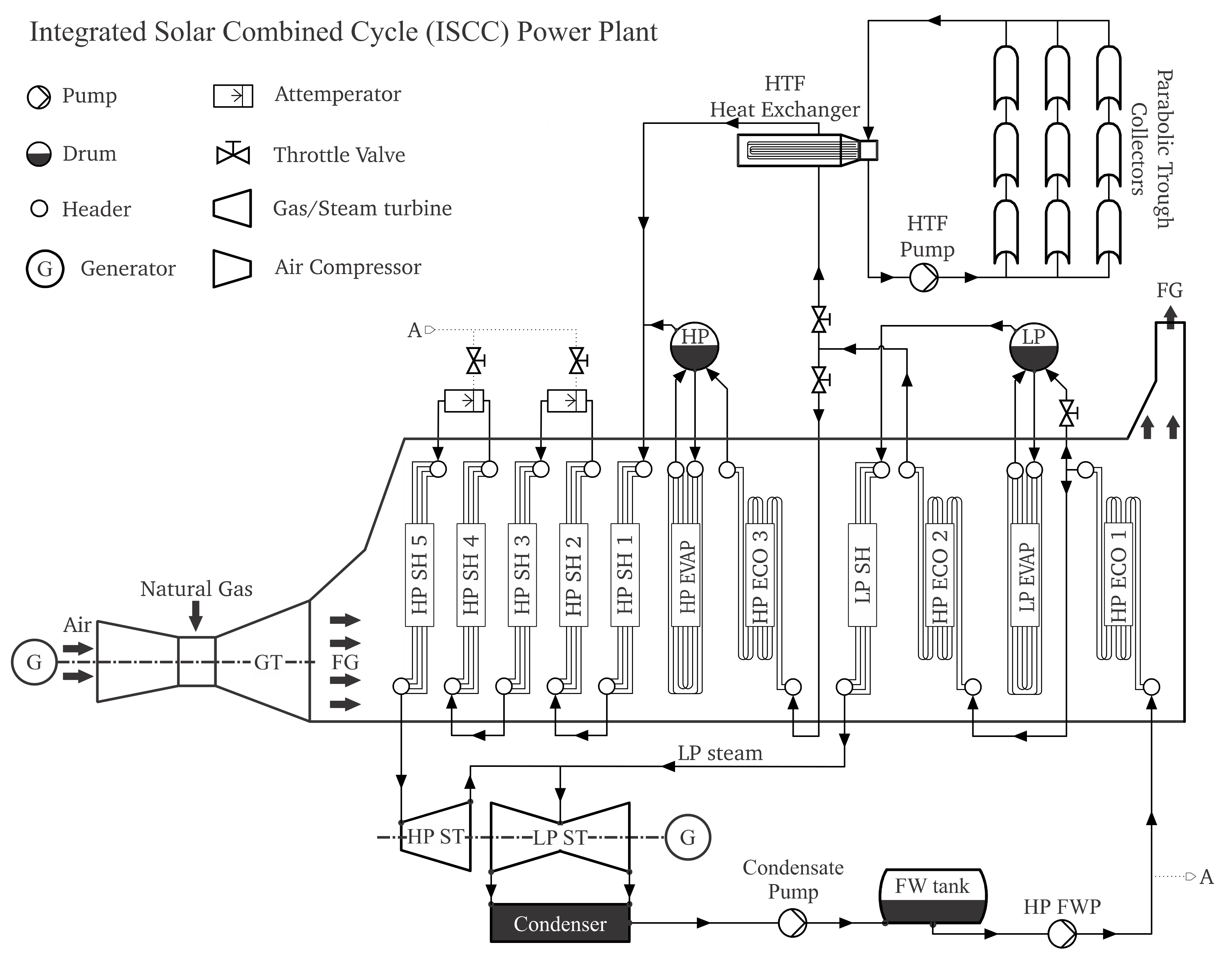
The plant has about 135 MW total electrical power output and includes a gas turbine (GT) with an electrical power output of 70 MW and a steam turbine (ST) with an electrical output of 65 MW [16,17]. It consists mainly of two parts: the solar field and the combined cycle, and the combined cycle is coupled with a parabolic trough collector solar field, as shown in Figure 1.

The solar field includes 160 parabolic trough collectors which uses the heat from the sun to warm up a heat transfer fluid (HTF) used to generate high-pressure (HP) steam in HTF heat exchangers (solar field heat exchangers). During the day, a part of the feedwater (FW) extracted from the heat recovery steam generator (HRSG) passes through the HTF heat exchangers, then this FW leaves the HTF heat exchangers as steam and is fed back to the HRSG where it is superheated.

In the combined cycle, the HRSG is located behind a GT, using the heat of the exhaust gasses from the GT to produce steam, which drives the ST and the generator (G). The objective of the HRSG is to use the hot exhaust gasses from the GT to heat water and convert it into (pressurized) superheated steam. The pressurized superheated steam expands in the ST, which drives a generator producing electrical power. At the rated output operating point, the GT supplies approx. 206 kg/s flue gases (FG) at a temperature of approx. 630 °C to the HRSG. The FG leave the HRSG system with a temperature of approx. 100 °C [18]. The enthalpy difference is transferred to the water-steam circuit to generate pressurized superheated steam.

The reference plant has two operating modes: day mode and night mode. During night mode, the solar field is shut down and the HRSG and the ST are operating at lower output mode. During day mode, the solar field is in operation and the generated steam is fed to the HRSG, then to the ST, which operates at a higher output mode. The load of the GT is approximately constant and independent of the operating mode (day/night mode).

3. Modeling of the Integrated Solar Combined Cycle

A full-scale dynamic model of the Kuraymat ISCC power plant is developed using the Advanced PROcess Simulation (APROS). It is a dynamic process simulator established for the representation of thermal power plant processes and the creation of realistic system-specific simulators. APROS is developed by the Technical Research Centre of Finland (VTT) and Fortum Nuclear Services Ltd. It contains component libraries for dynamic modeling of the process, automation and electrical systems, of thermal power plants, energy and industrial processes. APROS models for thermal power plant technologies are commonly found in the literature. Most models have been validated by actual measurement, which confirms the accuracy and readability of them, such as CCPP [19,20,21,22,23] and CSP plant [24,25,26].

The dynamic model is generated based on the piping and instrumentation diagrams of the existing 135MW_e ISCC power plant in Kuraymat, Egypt. All data of the construction geometry and the boundary conditions are from the plant. The reference plant includes three different circuits that are interconnected: the FG circuit, the HTF circuit, and the water-steam circuit. This structure, three different circuits, was mapped in APROS simulation to have a better view of the process and control structures. Therefore, the dynamic simulation model includes three different nets namely: the gas turbine net, the solar field net, and the HRSG net. Each net has its control structures and dynamic boundary conditions. The interfaces between the nets are the heat exchangers: the HRSG and the HTF heat exchangers. On the one hand, the HRSG consists of a setup of heating modules, which extract the heat from the FG and evaporate the water in the water-steam circuit. On the other hand, the HTF heat exchangers act as the interface between the solar field and the water-steam circuit in the HRSG by extracting the heat of the solar-heated HTF and transferring it to the water-steam circuit. The accurate functioning of these two interfaces is crucial to be able to achieve high-quality simulation results.

The standard process components of APROS libraries are used for the modeling (e.g., pipe, heat exchanger, and turbomachinery). The homogeneous flow model is used to describe the process components of the FG path and the water circuit, provided that the liquid and gaseous phases move through the system at the same flow rate and temperature. The point or node component is a basic process component that has at least one inlet and one outlet flow, and it is used to connect different kinds of process components. Between two connection points, the pipe component can be used to transport the working fluid and calculate the fluid flow (e.g., pressure drop, velocity). The specification of the pipe component includes the shape and dimensions of the pipes. The heat pipe comprises models for heat transfer between wall and fluid, heat storage into the tube and pressure loss of the flow, and it is used as a representation of different components in a power plant like pipes, valves, and heat exchangers.

The process control system shall be capable of handling the dynamics of the HRSG and HTF heat exchangers system without restricting the performance. Therefore, the developed model was controlled by implementing the real control structures and electrical systems from the reference plant.

3.1. The Gas Turbine Simulation

The gas turbine net simulates the compression of the air, the combustion, the subsequent expansion of the FG through the GT, and the heat transfer from the FG to the different heating modules of the HRSG, as shown in Figure 2. The FG mass flow is initialized from actual measurements as a boundary condition. The natural gas mass is controlled dynamically as these boundary conditions. The air flows into the compressor at ambient temperature, and pressure and its mass flow rate is specified as a dynamic boundary condition and controlled by the speed of the compressor. The compressor speed is controlled by a Proportional–Integral (PI) controller defined in APROS, which receives the mass flow behind the compressor as a variable and the mass flow from boundary conditions as a set point. The GT is defined under the assumption that the FG temperature, pressure, and mass flow match the actual measurements.

The FG from the GT, with a temperature of about 630 °C, is led through the inlet duct of the HRSG to the first heat transfer module (HP SH 5), and between the heating modules, intermediate ducts are installed, which allow entry between them. The last duct is the outlet duct, which connects the last heat transfer module to the stack, as shown in Figure 2.

3.2. The Heat Recovery Steam Generator Simulation

The HRSG net consists of a combination of heating modules, which extract the heat from the FG and evaporate the water in the water-steam circuit. The HRSG of the reference plant is a modular designed horizontal boiler with natural circulation. This means a horizontal FG direction with vertical tubes and natural circulation in the evaporators. As shown in Figure 1, the HRSG operates at two pressure levels. For each pressure level, water is supplied to the steam drum, via the economizers, by the HP feedwater pump (HP FWP). In the model, the condenser module is considered as dynamic boundary conditions.

The freshwater flows from the HP FWP into the first HP economizer (HP ECO 1) and is then divided into HP and low-pressure (LP) circuits. Before the HP ECO 2, a part of FW is extracted to pass through the LP evaporator (LP EVAP) and the LP SH, then to the LP ST. After the HP ECO 2 and before the HP ECO 3, a part of the FW is extracted to pass through the HTF heat exchangers during the day mode. The HP FW after the HP ECO 3 passes through the two HP evaporators (HP EVAP 1 and 2) and is then mixed with the steam coming from the HTF heat exchangers to pass through the five HP superheaters (HP SH 1, 2, 3, 4 and 5). In order not to exceed the maximum steam temperature of 556 °C before the HP ST and HP FW is injected through two attemperators, one attemperator is between the HP SH 2 and the HP SH 3, and another attemperator is between the HP SH 4 and the HP SH 5, as shown in Figure 1 and Figure 3.

In the HP water-steam path, the HP FW is heated in the HP economizers (HP ECO 1, 2, and 3) to a temperature close to the saturation temperature before it is fed to the HP drum. Then, the water from the HP drum is fed to the evaporators (HP EVAP 1 and 2) through the downcomer and is partially evaporated, as shown in Figure 1 and Figure 3. The driving force of the circulation is the difference of density between the water in the downcomer and the steam/water mixture in the EVAP tubes and risers, in so-called natural circulation. The saturated steam from the HP drum is fed to the HP superheaters (HP SH 1, 2, 3, 4 and 5) where it is superheated. Finally, the HP superheated steam, with pressure and temperature of about 70 bar and 566 °C respectively, is fed to the HP ST. The dimensions of the HRSG HP heating modules in the reference plant are given in

Table 1. Initialization of the HRSG high-pressure heating modules.

	HP Economizers			HP Evaporators		HP Superheaters
Module order	1	2	3	1	2	1	2	3	4	5
Number of parallel tubes in one row	41	41	41	41	41	41	41	41	41	41
Number of parallel rows	15	4	1	6	3	2	2	2	2	2
Outside diameter of the tube (mm)	38.1	38.1	31.8	38.1	44.5	44.5	44.5	44.5	44.5	44.5
Minimum tube thickness (mm)	3	3	2.6	2.6	2.6	3	2.9	3.2	3.6	3.6
Average tube length (m)	18.5	18.5	18.5	18.5	18.5	18.5	18.5	18.5	18.5	18.5
Outside diameter over fins (mm)	70.1	70.1	63.8	70.1	70.5	70.5	70.5	70.5	64.5	60.5
Thickness of the fins (mm)	1	1	1	1	1.3	1.3	1.3	1.3	1	1
Number of the fins (1/m)	280	255	120	280	280	280	280	280	250	120

.

The HRSG net has three main controllers: one regulates the HP FW mass flow rate of the HP ECO 1, another regulates the water level and the pressure in the HP drum, and the third controls the injection cooling upstream of the HP SH 3 and 5 (attemperators). The inlet of the HP FWP is specified as boundary conditions with a pressure of 11 bar and a temperature of 110 °C. The total FW mass flow rate is regulated via the manipulation of the main FW control valve.

3.2.1. The Level Control Mechanism of the HP Drum

The function of the drum level control is to adjust the level of the drum during the boiler start-up and to maintain its level at a constant steam load. A severe drop in this level can cause the boiler tubes to become exposed, causing them to overheat and become damaged. A rise in this level can disturb the process of separating moisture from the steam contained within the drum, reducing the efficiency of the boiler, and allowing moisture to be introduced into the process or turbine.

The ECO water is fed to the drum through a FW distribution tube, which distributes the FW evenly over the length of the drum, below the water level (setpoint). From the drum, the water circulates through the EVAP employing natural circulation. In the EVAP, a part of the water evaporates and the water-steam mixture returns to the drum, where it is separated into water and steam. Saturated steam leaves the drum from the top to the superheating modules, where it is superheated and finally flows to the ST. As mentioned above, the HRSG of the reference plant operates at two pressure levels [16,17].

The control mechanism of the HP drum regulates the mass flow of water into the drum. The LP control structures are almost similar to those of the HP circuit. The control system includes PI controllers defined in APROS, which control the water level and the pressure in the HP drum. The parameter to be controlled is the mass flow through the control valve. The control system of the HP drum level is based on a three-element control, as shown in Figure 4, which makes the controller more robust. The operation algorithm of the controller is described as follows:

• The deviation between the actual drum level (L_drum) and the setpoint drum level (L_setpoint) is determined and taken as an input signal for the PI controller.
• The difference between the mass flow rate of the FW and the produced steam ($\Delta \dot{m}$) is calculated.
• The sum of the signals ($\Delta \dot{m}$, ΔL) is used as the second input signal to the PI controller.

The PI controller regulates the FW mass flow into the drum through the continuous device control (DC) that regulates the FW mass flow rate from the FWP. As a basis for the control, the difference between the inlet and outlet mass flow of the drum and the change in the water level in the drum is measured and added. This sum defines the missing/excess water in the drum’s circulation system and is initialized as input to the PI controller. The PI controller aims to make the sum of the differences approach zero. The mass flow through the regulating valve is controlled by the output parameter of the PI controller (0 or 1). When the steam mass flow out of the drum increases and the water level in the drum decreases, the PI controller will increase the FW mass flow into the drum until the sum of the difference is zero. If the steam mass flow from the drum decreases and the water level in the drum increases, the PI controller reduces the FW mass flow into the drum until the sum of the difference is zero. In case the drum pressure exceeds a specific value (P_{max setpoint}), signal summation ($\Delta \dot{m}$, ΔL) is replaced by that resulting from the pressure difference between its pressure and its maximum pressure value, thereby preventing any further increase of its pressure. To avoid triggering the PI controllers with both signals at the same time, both output signals are filtered by a minimum filter defined in APROS. Both feedbacks (pressure and mass flow rate) controllers are connected to the minimum filter which selects both output signals and forwards the smaller value as input to the PI controller. This enables the PI controller to only be used for pressure regulation if the maximum permissible pressure is exceeded in the drum.

3.2.2. The Control Mechanism of the Attemperators

The attemperator is used to control the temperature of the superheated steam upstream of the ST by spraying water into the steam flow. The HRSG comprises two attemperators in the HP water-steam circuit to avoid the high-temperature difference in steam flow through the superheaters in the different operating modes (day/night mode). These two attemperators are located in front of two superheating modules, HP SH 3 and HP SH 5. The HP attemperators inject the FW mass flow at the inlet of the HP SH 3 and the HP SH 5, as shown in Figure 1, to continuously provide a constant steam temperature at the inlet of the HP ST. High fluctuations or spikes in the superheated steam temperature should be prevented to preserve the HP ST material for longer life. The attemperator is designed to ensure that all water injected into the steam is evaporated to prevent pitting of the turbine blades. The control mechanism of the attemperators regulates the superheated steam temperature at the outlet of the superheating section in order not to exceed the maximum permissible temperature of the HP ST (556 °C). The control system consists of a PI controller and control valve, defined in APROS. The input parameter of the PI controller is the measured temperature at the outlet of the last superheating module (HP SH 5). The temperature of steam at the outlet of the superheating section is measured and compared with the setpoint (in this case, 566 °C). The value of the difference between these two signals is the input signal for the PI controller. The PI controller regulates the mass flow through the attemperator’s control valve.

In the LP water-steam path, water extracted from the HP ECO 1 is led through a throttle valve to the LP drum as shown in Figure 1. In the LP drum, the water circulates naturally through the LP EVAP via a downcomer and is heated until the saturation temperature is exceeded. Then, the produced steam leaves the LP drum into the LP SH. The LP drum has a level and pressure control mechanism that is similar to that of the HP drum (Figure 4). Finally, the LP superheated steam from the LP SH is combined with the steam from the HP ST and is fed into the LP ST. The actual dimensions of the HRSG LP heating modules were used for dimensioning the HRSG tubes in the model and are given in

Table 2. Initialization of the HRSG low-pressure heating modules.

	LP EVAP	LP SH
Number of parallel tubes in one row	41	41
Number of parallel rows	6	1
The outside diameter of the tube (mm)	38.1	31.8
Minimum tube thickness (mm)	2.6	2.6
Average tube length (m)	18.5	18.5
Outside diameter over fins (mm)	70.1	-
The thickness of the fins (mm)	1	-
Number of the fins (1/m)	280	-

.

3.3. The Solar Field Simulation

The solar field comprises parallel rows of SKAL-ET 150 parabolic trough collectors forming 40 loops and each loop having four collector assemblies [27]. The mirrors cover 130,800 m² through 160 collectors and each collector has a total aperture area of 817.15 m², as shown in

Table 3. The solar field design parameters [27,28].

Solar Field Operation Parameters	Unit	Value
Total aperture area of the solar field	m2	130,800
Number of collectors per loop	N°	4
Number of loops	N°	40
Design DNI	W/m2	700
Maximum solar heat input	MJ/s	50
Output temperature of the HTF	°C	393
Input temperature of the HTF	°C	293

. The collectors are set up in a north-south direction and are rotated by a visual tracking system in an east-west direction to align the collector mirrors towards the sun depending on the angle of incidence. The solar field based on the HTF system delivers about 50 MW (thermal) at full-load operating conditions. The HTF is heated in the receivers of the solar collectors and transfers its absorbed thermal energy through the HTF heat exchangers to the water-steam circuit. The HTF used in the solar field is a liquid phase HTF (Therminol VP1) [16,17]. The HTF heat exchange system includes two similar parallel trains, each train consisting of an ECO and an EVAP in series. Both ECO and EVAP are shell and tube type heat exchangers with water-steam on the shell side and HTF on the tube side, U-tube type.

The heat absorption by the parabolic trough collectors is modeled in APROS through heat pipes in the solar field net, as shown in Figure 5. The effects of the solar field were mapped, and a wide variety of influences (shading, activation, and deactivation) are modeled through the simulation. Each heat pipe simulates a parabolic trough solar collector, and every four heat pipes form a loop. Each loop inlet is connected to a cold header and the loop outlet is connected to a hot header. The solar field net includes 40 loops in total divided symmetrically in two solar fields, east and west fields. The DNI is dynamically initialized in each heat pipe via boundary conditions and heats the HTF flowing through. The absorbed incident solar radiation (${\dot{Q}}_{inc}$) is given by:

$${\dot{Q}}_{inc}=DNI\ast cos\theta \ast IAM\ast A_{mirrors}$$

(1)

where,

• $\theta$ = the incidence angle [degree].
• $IAM$ = the incidence angle modifier [-].
• $A_{mirrors}$ = the aperture area of the solar collectors [m²].

Where the incident angle modifier ($IAM$) is a correlation of the collectors’ losses due to extra reflections and the heat absorptions by the glass envelope and it can be obtained as follows:

$$IAM=1+\frac{0.000884\ast \theta }{\cos \theta }-\frac{0.00005369\ast {\theta }^2}{\cos \theta }$$

(2)

and the aperture area of the solar collectors ($A_{mirrors}$) is obtained as follows:

$$A_{mirrors}=N_{collectors}\ast W_{collector}\ast L_{collector}$$

(3)

where,

• $N_{collectors}$ = the number of solar field collectors [-].
• $W_{collector}$ = the width of the collector [m].
• $L_{collector}$ = the length of the collector [m].

All solar field losses (receiver losses, cleanness losses, shadow, incidence angle, etc.) and the parabolic trough collector’s optical efficiency are considered in the calculation of the solar heat absorbed (${\dot{Q}}_{Solar}$) [27]. The solar heat absorbed (${\dot{Q}}_{Solar}$), defined as solar heat input, was multiplied by the aperture area of the solar field (130,800 m²) and divided by the number of solar collectors (160), then the resulting value is initialized into the heat pipes as the heat to be absorbed by the HTF.

Figure 5. Schematic of the solar field net in APROS.

Figure 5. Schematic of the solar field net in APROS.

The HTF system is responsible for delivering the solar heat gained by the HTF (${\dot{Q}}_{Solar}$) [27] to the water through the HTF heat exchangers. The solar field net includes the HTF heat exchangers that act as the interface between the solar field net and the HRSG net (water-steam circuit). The accurate functioning of these HTF heat exchangers is crucial to be able to achieve accurate simulation results. HTF heat exchangers are used to generate steam by cooling the HTF coming from the solar field, and this HP steam is fed back to the HRSG and is combined with the steam from the HP drum.

The main HTF pumps are variable speed pumps with a design mass flow of 250 kg/s that varies between 30 and 100% according to the actual solar irradiation. As a function of the mass flow rate, the pressure drop in the HTF cycle varies in a wide range between 1 to 15 bars. The HTF pumped into the solar field is equally divided into two streams between the east and the west fields by control valves, as shown in Figure 5. The FW is supplied from a draw-off inside the HRSG ECO system, as shown in Figure 1. The FW from the HRSG is preheated in the HTF ECO up to just below saturation before entering the HTF EVAP. In the HTF EVAP, steam is generated by cooling the HTF flow from the solar field as in the HTF ECO. The ECO and the EVAP are both shell and tube heat exchangers with two tube paths, type U-tube, as in

Table 4. The specifications of the HTF heat exchangers.

Parameters	Unit	Shell Side	Tube Side
Fluid	-	Water/Steam	Therminol VP-1
Nominal fluid flow rate	Kg/s	28.5	173.25
Inlet temperature	°C	288.66	393
Outlet temperature	°C	291.66	292.93
Inlet pressure	bar	76.311	17
Nominal velocity	m/s	0.47	1.81
No. of passes per shell	-	1	2
No. of tubes	-	1110U
Gross surface area	m2	1034.05
Effective shell/unit area	m2	1006.37
Mean temperature difference	°C	23.7

. The steam coming from the HTF heat exchangers is combined with the steam coming from the HP drum and flows further into the HP SH 1, as depicted in Figure 1 and Figure 3.

The solar field net comprises three control systems that regulate the HTF mass flow into the solar field, and the mass flow rate of the HTF and the water into the HTF heat exchangers. The first control system regulates the HTF mass flow through a PI controller defined in APROS to reach a constant outlet temperature (393 °C) from the solar collectors in order not to exceed the maximum allowable temperature of the HTF (400 °C). The second control system regulates the cooling mechanism of the HTF in the HTF heat exchangers through a bypass system to maintain the HTF inlet temperature to the solar collectors at 293 °C. In the night mode (no solar heat input), the HTF flows through a bypass control valve and circulates in the solar field to prevent the HTF from entering the HTF heat exchangers—this avoids undesired cooling of the HTF by the water in the HTF heat exchangers waterside. The third control system regulates the FW mass flow in the HTF heat exchangers through a PI controller to reach the saturation temperature of the water at the outlet of the HTF heat exchangers.

3.3.1. The Control Mechanism of the HTF Mass Flow

The HTF mass flow into the solar field is divided equally between the east and west fields by two control valves. The HTF mass flow control system adapts the HTF pump speed to maintain the HTF outlet temperature from the solar field at 393 °C in order not to exceed the maximum allowable temperature of the Therminol VP1 (400 °C). The HTF mass flow control system includes a PI controller defined in APROS that controls the speed of the HTF pump depending on the heat rate absorbed by the HTF in the solar field (${\dot{Q}}_{Solar}$).

The variable to be controlled is the HTF mass flow rate that is measured before the HTF pump. The required mass flow (${\dot{m}}_{required}$) to be achieved is determined in a calculation cascade as follows:

• Calculating the specific enthalpy of the HTF at the solar field inlet (h_in) from the measured pressure (P_in) and temperature (T_in).
• Calculating the specific enthalpy of the HTF at the solar field outlet (h_out) from the measured pressure (P_out) and the set point temperature of 393 °C.
• Calculating the required HTF mass flow rate (${\dot{m}}_{required}$) to reach the HTF temperature of 393 °C at the outlet of the solar field by dividing the heat rate gained from the solar field (${\dot{Q}}_{Solar}$) by the specific enthalpy difference between the calculated specific enthalpies (h_out and h_in), as shown in Figure 6.

The HTF mass flow (${\dot{m}}_{required}$) is compared with the measured HTF mass flow rate before the HTF pump (${\dot{m}}_{HTF}$). The difference between the two mass flow rates is initialized as a setpoint into the PI controller. Then, the output parameter of the PI controller regulates the output of the HTF pump between 0%–100% with a maximum mass flow of about 250 kg/s.

3.3.2. The Control Mechanism of the HTF Bypass

The HTF bypass mechanism regulates the temperature at the inlet of the solar field through a bypass system. The reference plant has a complex system to cool the HTF. In the model, the HTF cooling is achieved via two heat exchangers in series (ECO and EVAP) of counter flow type, as shown in Figure 5. The enthalpy difference of the HTF between the solar field inlet and outlet is transferred to the water-steam circuit via the HTF heat exchangers. The water coming from the HP ECO 2 is evaporated and slightly overheated in the HTF heat exchangers and then flows into the HP SH 1 with the steam from the HP drum, as shown in Figure 1 and Figure 3. The HTF bypass system activates and deactivates the HTF mass flow into the heat exchangers and ensures a constant HTF outlet temperature from the heat exchangers at 293 °C. A PI controller, defined in APROS, measures the outlet temperature downstream of the HTF heat exchangers and controls the mass flow through the bypass valve, thus the HTF inlet temperature to the solar field is constant (293 °C). If the outlet temperature drops below 293 °C, the PI controller bypasses the HTF heat exchanger by partially opening the bypass valve. Thus the HTF outlet temperature from the HTF heat exchangers is controlled to a constant 293 °C. When the temperature at the solar field inlet is above 293 °C, part of the mass flow is cooled in the heat exchangers via a control valve.

3.4. Dynamic Boundary Conditions

In the dynamic model, boundary conditions were initialized for the GT, FW and DNI parameters as a function of time. All boundary conditions were initialized as hourly values and timed by a common timer defined in APROS. A polyline module defined in APROS is used to interpolate the initialized time values into a polynomial curve. To calculate different time series (different days), a switch defined in APROS can switch between different initialized polylines. In the gas turbine net, the boundary conditions for the natural gas and the combustion air were initialized. The natural gas temperature and pressure of 22.5 °C and 1 bar, respectively, were initialized as constant values as applied in the reference plant. The FG mass flow was initialized in a PI controller to regulate the pressure and the mass flow rate of the compressor through its speed. In the HRSG net, the pressure and the temperature boundary conditions for the FW coming from the HP FWP were initialized in the node module before the HP ECO 1. Finally, the DNI was initialized in the solar field net according to the actual measurements.

4. Results and Discussion

The developed model is tuned using the operational design data of the reference plant. A comparison between this data and the simulation results was presented and evaluated. Then, the dynamic simulation is implemented and its results are compared with actual measurements.

4.1. Model Tuning

The steady-state simulation is just one initial condition for a dynamic simulation to tune the model. To increase the validity of the steady-state verification, it is performed for two different cases. As indicated in

Table 5. Reference steady-state cases description (operational design data).

Parameter	Case 1	Case 2
Ambient temperature (°C)	20	35
Natural gas flow rate (kg/s)	4.71	4.33
FG mass flow rate (kg/s)	206.36	190.47
FG temperature (°C)	605.29	622.94
Solar heat input (MW)	50	50
Net electrical power output (MW)	129.251	116.62
Net power plant efficiency (-)	60.93	59.77

, the model was tuned using the operational design data for 50 MW solar heat input, and two different ambient temperatures of 20 °C and 35 °C [16,17].

The model was iteratively improved so that the numerical results match the operational design data of the two reference cases. The boundary conditions of the GT, the FW and the DNI were initialized with constant values. The steady-state simulation results were calculated and compared with design data, and the accuracy of the main parameters’ results was evaluated and presented in

Table 6. Comparison between the simulation results and the operational design data.

Parameter/Variable	Case 1			Case 2
	Reference	Simulation	Error	Reference	Simulation	Error
FW inlet temperature to the solar field (°C)	236.59	235.20	0.59%	232.86	231.49	0.59%
FW mass flow to the solar field (kg/s)	28.79	28.34	1.57%	28.48	27.89	2.09%
FW outlet temperature from the solar field (°C)	293.90	300.68	2.31%	292.56	299.17	2.26%
FG temperature (°C)	605.29	604.46	0.14%	622.94	604.46	2.97%
FW mass flow after FWP (kg/s)	56.80	56.81	0.01%	49.25	48.98	0.55%
FW pressure after FWP (bar)	150.40	149.99	0.27%	150.80	150.40	0.27%
Steam pressure in LP drum (bar)	10.91	11.21	2.71%	10.82	10.77	0.48%
FW mass flow before LP drum (kg/s)	3.85	3.85	0.0%	3.30	3.39	2.72%
Steam pressure after LP SH (bar)	10.22	10.77	5.40%	10.22	10.41	1.89%
Steam temperature after LP SH (°C)	232.70	232.71	0.01%	235.40	232.98	1.03%
Steam pressure in HP drum (bar)	76.24	80.07	5.03%	74.57	78.28	4.97%
Steam mass flow before HP ST (kg/s)	46.78	46.52	0.55%	45.95	45.59	0.78%
Steam temperature before HP ST (°C)	559.70	560.01	0.06%	559.39	560.26	0.16%
Steam pressure before HP ST (bar)	69.38	67.81	2.26%	68.33	66.48	2.71%

.

As indicated in Table 6, the simulation results match the operational design data with high accuracy. Less accuracy appeared in the simulation pressure values (steam pressure after LP superheater and steam pressure in HP drum). The reason for these differences may be due to the geometry of the heat exchangers. Since the geometrical data is given in the model, further optimization of the pressure values is difficult. After the model was tuned and verified, the simulation environment is initialized with the dynamic boundary conditions, as will be explained in detail in the following sections.

4.2. Dynamic Model Validation

After the tuning of the model using operational design data for two different ambient temperatures, as indicated in Table 6, it is necessary to find out if the model can reproduce the dynamic behavior for temperature, pressure, mass flow, and power of the reference plant. Here, the dynamic model is validated using actual measurements for four different days in three different months: 20 July 2013, 21 July 2013, 30 August 2013 and 4 September 2013. The main difference between the simulation days is the incoming DNI into the solar field and the resulting total electrical power outputs from the GT and the steam turbines in addition to the different ambient conditions. For the dynamic simulation, dynamic time series over 24 h were available for each day. The dynamic simulation results for the heat absorbed from the given DNI values of different days were simulated, then the mass flow rate, temperature and pressure values along the power plant were presented and compared with the actual measurements. Here, it should be mentioned that the model is not tuned during the dynamic simulation for the different given days.

Figure 7 shows the measured and simulated heat gain from the solar field for four selected days. The DNI is provided here for reference. The heat rate (${\dot{Q}}_{Solar}$) shown in the figure is normalized on a per unit solar field aperture area basis, so the unit is (W/m²). The DNI is the main factor determining the solar heat harvested by the HTF in the solar collectors (${\dot{Q}}_{Solar}$).

The calculation point of the HTF heat absorption rate (${\dot{Q}}_{Solar}$) simulation results are shown in Figure 7 and are located at the outlet of the solar field, directly before HTF heat exchangers. The simulation results show agreement with measured data, and this behavior is mainly achieved by the control system defined in the model.

In the HRSG net, the simulation of the HP and LP water-steam circuits and the simulation of the steam coming from the HTF heat exchangers are of particular importance. Besides, it is necessary to check whether the simulation can approximate the mass flow of the FW in both HP and LP circuits. Figure 8 reveals the simulated and the measured FW mass flow in the HP and LP circuits for the four different days.

In Figure 8, the FW mass flow in the HP circuit increases during the day as a result of the availability of the solar field in the power plant, contrary to the FW mass flow in the LP circuit, which decreases slightly during the day. Figure 8 indicated that the simulation results of the FW mass flow rate for both the HP and the LP circuit match well with the actual measurements for the four different days. During the day mode, the additional FW mass flow in the HP circuit is well represented. The results showed that the FW flow in the LP circuit decreased during the daytime mode, which could be due to the decrease of available heat in the FG due to the higher mass flow in the HP circuit, and this slight decrease was also well represented with the simulation results. The fluctuations of the mass flow are modeled, but its extreme rates of change cannot be modeled accurately, however, a good trend is observed. The measuring point of the HP and LP FW mass flow is located upstream of the HP ECO 2 and upstream of the LP drum, respectively.

Figure 9 shows the simulated and the measured steam mass flow rate after the HP SH 5 and the LP SH. Similar to the FW mass flow, the steam mass flow in the HP circuit also increases during the day, contrary to the steam mass flow in the LP circuit, which slightly decreases during the day. Figure 9 revealed that the simulation model can accurately represent the trend of steam mass flow change after the HP SH 5 and the LP SH. Again, the increased mass flow in the HP circuit and its decrease in the LP circuit during the day can be modeled well, but the representation of the extreme values cannot be modeled identically; however, a good tendency can be seen.

Figure 10 shows the simulated and the measured steam pressure before the HP and LP steam turbines. The actual measurements show that the pressure of the steam after the HP superheating modules significantly increases during the day. The simulation results are slightly higher than the actual measurements, especially at the extreme values, however, the model can simulate the steam pressure variation during the load change well.

In contrast to the actual measured data of the LP steam, constant pressure is observed in the simulation results which can be attributed to the measurement point and the role of the pressure control mechanism of the LP drum (Figure 4). The measuring point prevented the effect of the solar field-induced pressure change through a control valve upstream of the ST. It is possible to reproduce the effect of the solar field-induced pressure change by moving the measuring point between the control valve and the ST.

Figure 11 shows the simulated and the measured temperature behavior of the superheated steam after the HP SH 5 and LP SH. The effect of the solar field can be seen here in the temperature values of the LP steam. The steam temperature in the LP circuit increases during the day which may be due to the decrease of the LP mass flow during the day. The results show that the temperature behavior of the actual measurements can be reproduced by the model. In Figure 11a,b, the actual measurements of the days 20 July 2013 and 21 July 2013 show that the temperature of the HP steam before the ST decreased during the day, however, the model reproduced the temperature value with a constant value which is due to the control mechanism of the constant steam temperature before the ST through the attemperators. It is not recommended to change the steam temperature before the steam turbines, as this may cause material problems in the blades of the ST. The simulation results reveal the role of the attemperators in controlling the steam output temperature from the superheating modules, HP SH 5 and LP SH, in the dynamic model.

The last important parameter to be validated is whether the overall performance of the ISCC systems can be simulated by the electrical power output of the ISCC power plant. Figure 12 shows the simulated and the measured electrical power output from the steam turbines and the whole ISCC power plant. Unlike the stand-alone solar power plant, the ISCC power plant produces electrical power for the grid regardless of solar radiation conditions, as revealed in Figure 12. During the day, the electrical output of the ISCC power plant is increased as a result of the heat harvested in the solar field. It can be concluded that the curve of the measured electric power output can be simulated well through the dynamic model.

During the day, the simulation results represent the actual measurements of the steam turbines’ electric power output with high accuracy. There are small deviations in the simulation results for the electric power output of the whole ISCC power plant which is due to the deviation in the simulation results for the electric power output of the GT.

5. Conclusions

A dynamic process simulation model of an existing ISCC power plant was developed using APROS simulation software. The model was initialized and tuned using the operational design data from the reference plant. In addition, the main control mechanisms for the drums, control valves, and solar field have been implemented. The dynamic model represents reality with high accuracy and forms a good predictive capability for future dynamic simulations. All components including the solar field, the HRSG and the controlling structures were modeled with the actual specification data from the reference plant. Then, the dynamic simulation was performed for four different days and the simulation results are compared with the actual measurements. The simulation results of the heat absorption by the HTF in the solar field for four different days were presented and compared with actual measurements. Then, the FW mass flow rate and the mass flow rate, the pressure and the temperature of the steam before the steam turbines were also simulated and compared with their actual measurements. Finally, the electrical power output from the steam turbines and the whole ISCC was calculated and compared with its calculation from the actual measurements for four days. The comparison study showed that the developed model reproduces accurately the most important parameters in the plant (pressure, temperature, mass flow, and electrical power output). The developed model was only tuned using the operational design data and no further tuning was considered during the dynamic simulation. The simulation environment was able to depict the behavior of an ISCC power plant very well and can be taken into account in future planning decisions. Finally, it should be mentioned here that the validated dynamic model is of high relevance for the design and operational flexibility of the ISCC power plant to guarantee an affordable and secure supply of electricity.