1. Introduction
The economic growth and improvement in living standards depend on the utilization of electrical energy. This growing demand for electrical energy whilst trying to reduce environmental pollution is one of the main reasons why we are advocating for the advancement and implementation of renewable sources in both urban and rural areas. Hydropower is one of the favorable renewable energy sources required to fulfil future energy demand. However, according to the deep history of hydro technology, many large-scale hydro opportunities using dammed reservoirs have already been exhausted. Therefore, small-scale hydropower has a high tendency to exploit unused resources such as rivers or streams [
1,
2].
The Archimedes screw turbine (AST) represents the most sustainable small hydropower extraction method as it is economically, socially, and environmentally beneficial. As a clean and renewable energy source, AST has a minimum impact on wildlife, especially fishes that can pass through with minimal harm [
3]. Many studies indicate that low-head hydropower facilities have less impact on river ecosystems and eventually provide environmental benefits [
4]. Thus, AST power plants claim relatively high efficiency with lower installation and maintenance costs than the other small-scale hydropower extraction methods with reduced economic benefits. The simplicity of the AST structure is one of the main advantages of the manufacturing process, greatly reducing the manufacturing costs. Simultaneously, AST was identified as the best solution to generate electricity for undeveloped regions and areas, especially high elevations of mountains or small communities far from facilities and infrastructure. In the aspect of social benefits this is an important advantage for remote communities where central grids are neither accessible nor cost-effective [
3].
The history of the rotating screw dates back to the Egyptian civilization era where it was used as an irrigation pump on the Nile River. The Roman engineer Vitruvius gave a detailed description of the construction of an Archimedes screw in the first century [
5]. Radlik introduced the use of the Archimedes screw as a turbine for energy conservation, and the first AST was installed in 1997 on the Eger river in Germany [
6]. Since Brada’s [
7] and Nuernbergk’s [
6] pioneering work, ASTs have been rapidly adopted and there are now hundreds of installations, almost entirely located in Europe, providing power to the grid.
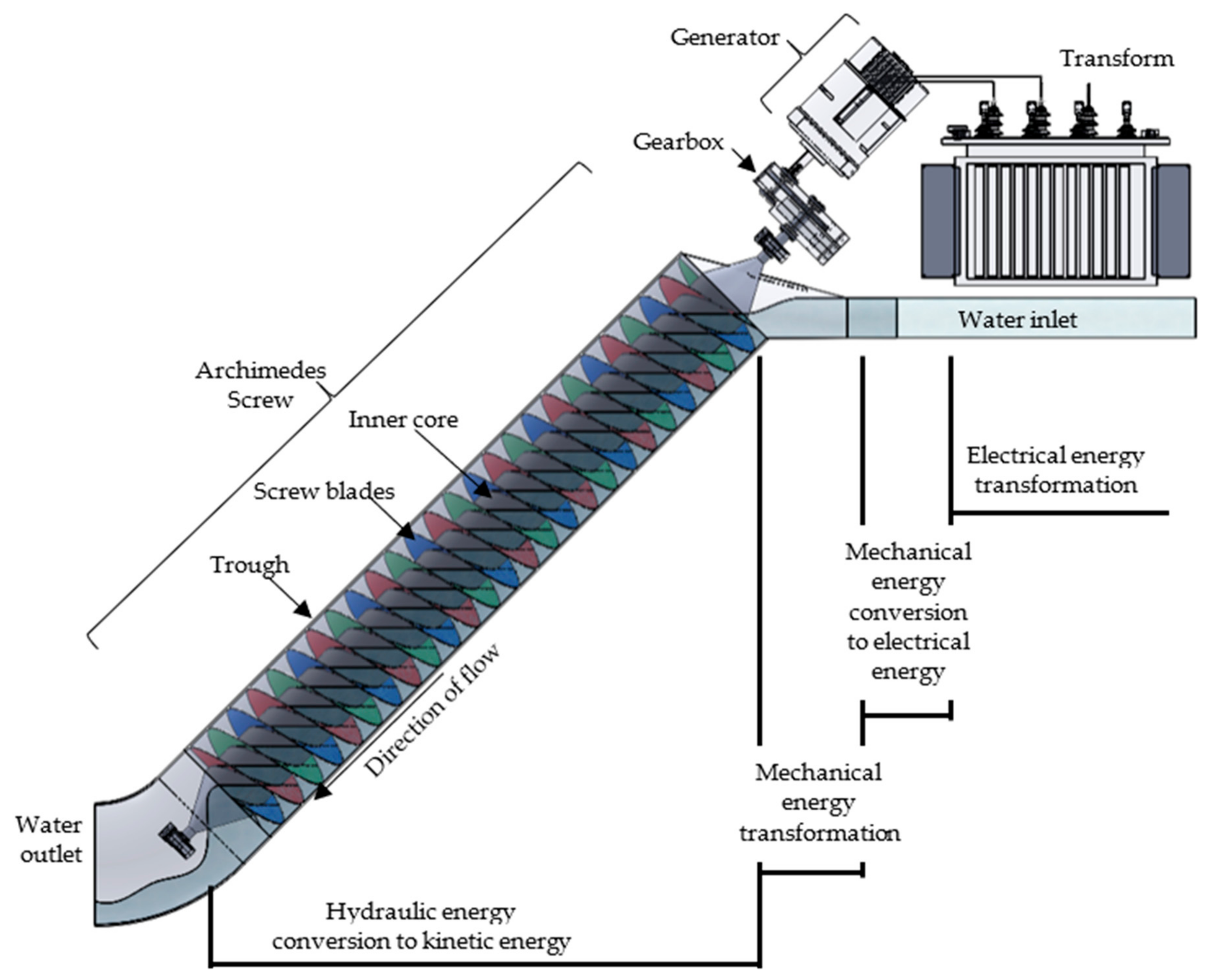
Energy conversion in an AST begins with the potential energy of water being converted into kinetic energy in the screw and then converted into electrical energy using a generator. As shown in
Figure 1, the screw exerts kinetic energy because of the rotary motion generated by torque on the screw blade due to the hydrostatic pressure difference. Thereafter, it is converted into a suitable rotation speed via a gearbox which is suited for the generator. Therefore, the mechanical energy loss which occurs can be estimated by the mechanical efficiency. Then, using a generator, the mechanical energy is converted into electrical energy with a certain electrical efficiency. In the AST design process, the basic and the most important part is the conversion of hydraulic energy into mechanical energy inside the screw.
The operating principle of the AST is different from that of other types of hydro power turbine. The AST is mainly driven by the hydrostatic pressure differences that develop across the screw surfaces due to the weight of the water volume which are at different water levels within the inclined screw [
8].
Figure 2 illustrates how the pressure is generated by different water levels. This energy conversion is totally different from the impulse type (Pelton turbine) or reaction type (Kaplan turbine) hydro turbines. The AST energy conversion method is closer to the technology of water wheels which have as long a history as Archimedes screw pumps.
The AST structure consists mainly of helical screw blades, which are fixed to a center core. This whole region is called a screw and it is free to rotate on its center axis. There can be N number of screw blades attached to the center core, with a constant screw pitch. Most researchers claim that three screw blades are more suitable since they result in good performance as well as being easy to manufacture. This screw structure is then laid in a channel with a semi-circular or even closed circular cross section [
8] called a trough, having a clearance gap between the screw blade tip and the inner wall of the trough.
The water volume enclosed by the trough and the nearby two screw blades are called a water bucket. The total water volume inside the AST is then equal to the number of pitches into water volume in a bucket (volume of the total number of water buckets) [
5].
With the assumption of no leakage flow, available water flow rate should be compatible with the nominal flow rate which contributes to generate power inside the AST. Usually, there are two main aspects of leakage losses – gap leakage and overflow leakage. Gap leakage is identified as the flow through the clearance gap between the blade tip and trough, while overflow leakage is identified as the flow over the center core when the screw operates under overfilling conditions. Therefore, in a real AST, the available flow is equal to the sum of the nominal flow and the leakage flows. These leakages are identified as a power loss since water passes through the screw without contributing to the power generation [
2]. By reducing these leakage losses, the AST performance can be improved. Maintaining the minimum possible clearance gap is the key factor to reducing the gap leakage loss. There is an optimal rotational speed of AST, which reduces the overfilling phenomena, and hence, reduces the overflowing leakage loss.
Other than the leakage loss, there is a frictional loss due to the viscous shear force along the blade surface, shaft and the trough inner wall [
9,
10]. When the screw is lengthier, the frictional loss becomes significant. One of the methods to reduce the fictional loss is to manufacture smooth quality surfaces in the AST.
There are not many well-known things about ASTs, thus the need to increase the rate of research on these machines [
5]. Currently, there is no perfect theory or rule for the optimal hydraulic design of ASTs, and their hydropower plants are highly dependent on the experience of the design engineer. Thus, there is no sufficient guidance in English for the optimum design procedure of ASTs, as the existing literature is almost entirely non-English [
7,
11]. Many researchers used the Nuernbergk charts in their AST design procedures, as it is the best and latest source of literature that considers both leakage and frictional losses [
6]. Since that report is in German [
3], the usage of the report is limited, but an English translation of Rorres’s report can be used, which includes the optimized parameter ratios for Archimedes screw pump design, which were improved recently by Nuernbergk for the design of ASTs [
2]. Most researchers do not describe the design procedure of their ASTs. But those studies are important as they mainly focus on specific AST parameters such as screw inclination [
7], pitch, gap leakage, overflowing leakage [
12], bucket filling ratio [
2], diameter ratio, and many other factors considering the AST performance while enhancing its advantages, therefore essentially designing a new AST where its suite of parameters for a specific site is an issue. This study addresses this issue by focusing on designing a new AST based on Rorres’s report while calculating all dimensions using the optimal ratios.
Most of the AST arrangements are made up of smaller upper and lower reservoirs. The upper reservoir’s water level is automatically controlled by the rotational speed of the screw for the available inlet flow rate. The lower reservoir’s water level significantly affects the efficiency of the AST. When the screw outlet is not immersed in water, it does not exert back-pressure on the last screw turn. Therefore, the pressure due to the water filling at the last screw turn is greater, and the extracted power becomes higher. But other than that, non-immersion results in a high hydraulic head and, consequently, relatively higher available power, hence reducing the hydraulic efficiency. Therefore, it was observed that the 0.6 immersion ratio at the outlet is the optimum water level which maintains the highest efficiency of an AST [
13]. Generally, run of river hydro systems without any reservoirs are highly beneficial to the environment, but an AST plant without reservoir raises the problem of maintaining high efficiency, especially without controlling the down reservoir water level. Therefore, this research focuses on developing an AST inner design that results in high efficiency even in the absence of reservoirs.
Most AST studies have a primary focus on experiments, especially using small-scale lab test models [
11]. Very few studies on CFD models of ASTs are validated by experiments. Dellinger’s study is a reliable simulation study with validation through experimental models [
6], which is extensively referred to in this study. Thus, many researchers are limited to small-scale AST simulations due to computational power limitations during CFD simulations. However, CFD can simulate large AST models on the real scale by utilizing appropriate computational facilities and this study describes a simulation technique for a real scale AST.
Conventional ASTs are driven by the hydro potential energy, where the hydraulic head is significant, but nowadays AST are being investigated as hydrokinetic turbines where the turbine is driven using the velocity of the water [
14,
15]. Those ASTs can work fully horizontally or have small inclinations [
16] where there is a significant velocity of free-flowing water, especially in rivers. For hydro potential ASTs, many researchers claim 80% efficiency for low inclinations of about 25–30 degrees. High inclination ASTs are considered as less efficient because of the energy loss due to the leakage and bubbled vortex flow [
17]. On a real scale, AST designs for small inclinations result in lengthy screws that screws may cause problems with bending, bearing limitations, and high frictional losses [
2]. For those sites it is recommended to install two or more steps by step screws, but that approach has high initial costs. Those specific sites could be equipped with high inclination ASTs, which tend to reduce the frictional losses while maintaining 80% efficiency. The current study was done to address this problem by examining the computational flow field and numerical performance for a real scale run-of-river AST arrangement with the highest possible inclination of 45 degrees.
Finally, this study discusses the suitability of Rorres’s optimal design ratios and the CFD simulation for a real site scale AST that can achieve high efficiency even at a 45 degree high inclination without any reservoirs.
2. Methodology
2.1. Design Procedure
Initially, the AST design was done to operate at the drainage water flow in a fish farm near the east sea of South Korea. Fish farms usually circulate the fresh seawater by pumping from the sea and discharging the tank water. Pumping water may consume power, and discharge water is considered as the wastage of energy. Therefore, this waste energy can be captured to use light-duty applications such as lighting the fish farm itself. In this analysis, the fish farm’s drainage pipe outlet is situated at about 5.5 m above sea level. The available average flow rate was estimated at 0.232 m3/s. Considering the AST installation site, a run-of-river system was recommended. A pipe connection was introduced to connect the drainage pipe to the screw, instead of an upper reservoir. Furthermore, the lower reservoir was omitted since the sea water level is unpredictable due to sea waves and tides. Due to the absence of reservoirs, the AST design is presumed to have a relatively low efficiency. After determining the AST installation outline, the optimum dimensions for the AST were calculated according to Rorres’s optimized parameters. Thereafter, a 3D solid model of the screw was built up in SolidWorks. Then the fluid domain was modeled in SOLIDWORKS 2016 and meshed in Ansys ICEM CFD 19.2 version. Finally, the setup was built in Ansys CFX 19.2 version and the CFD was solved for the fluid domains. Thus, the desired parameters were calculated in order to evaluate the performance of the AST. Then, the Ansys postprocessing was used to analyze the flow behaviors.
Dillinger’s small-scale AST study was used to validate the current CFD setup, as his research claimed good agreement between CFD and experiment results. Results are in reasonably good agreement with the reference study as highlighted below in the Results and Discussion section.
Rorres’s study, which was used to design the new AST, was originally done to optimize an Archimedes screw pump, but it is assumed to be suitable for AST design since the optimization is based on lift-up of the maximum water flow [
18,
19]. On the other hand, AST optimization is focused on maintaining a high-pressure difference on screw blades, which is determined by the difference in water level, when an optimum water volume exists within the screw buckets. This optimum water volume is determined as a bucket volume ratio. Therefore, Rorres’s optimized ratios [
5] are compatible to use for the AST design.
In Rorres’s report, the parameters are categorized as external and internal parameters. Outer radius, screw length and the slope of the screw are the external parameters. These external parameters are dependent on the installation site (flow rate, available head and space) and the manufacturing capability of screws. Inner radius, screw pitch and the number of screws are the internal parameters. Depending on the external parameters, the internal parameters should be optimized in order to increase the performance of the AST. Initially, three screw blades were selected for this design considering the manufacturing limitations, especially the cost. It was also revealed that the three number of screw blades result in high water level difference [
6] along the AST blades for a wide range of flow rates.
Since the available hydraulic head is 5.5 m, we selected a 45 degrees slope for the design of the AST, while maintaining the minimum possible screw length. The minimum possible screw length is calculated as 7.78 m. Furthermore, using the Rorres’s optimum volume per turn ratio for three bladed screws, the outer diameter of the screw was calculated using Equation (1):
where
is the maximum water volume in one screw cycle, where the screw is large enough to hold the available flow rate within one cycle of rotation. The ratio of water volume per cycle to the available flow rate can be varied considering the screw’s operating rotational speed and the compatibility of the screw size.
is the Rorres’s optimum volume per turn ratio which equals 0.0598.
is defined as
, where
is the slope of AST to the horizontal direction.
is the outer radius of the AST which is calculated as 1.16 m which was rounded off to 1.2 m.
Then, using the optimum diameter ratio
for three bladed screws, the inner diameter
was calculated as 0.643 m:
Also, using the optimum pitch ratio
for three bladed screws, the screw pitch
was calculated as 0.836 m:
It was found that about eight numbers of turns are compatible along the 7 m screw length with 0.836 m pitch length.
Hence the internal parameters were calculated, thanks to the Rorres’s optimum ratios. Then comparing it with the previous small scale AST blade’s thickness, it was determined to be 0.005 m thickness. The gap between the blade and the trough
was determined as 0.005 m using the Equation (4) recommended by the Julien study [
2]:
For the final design, the rotational speed was calculated as 54.58 rpm which is almost equal to the available flow rate passing through the one screw cycle rotation, as described in Equation (5) [
6]:
where the
is flow rate through the screw and
is the screw rotational speed in rpm.
Moreover, screw is designed with a fully covered trough, since the 45 degrees high inclination can result in more turbulent flow. Thus, fully covering the trough makes the AST simulation easier to solve. Since the drainage pipe diameter is 0.4 m, the connection pipe was designed to guide the water flow into the screw as shown in
Figure 3.
The top surface of the connection pipe was open to atmosphere allowing the screw to operate under atmospheric pressure. At the outlet of the AST, another pipe segment was added allowing the water to flow out. Hence the down reservoir was omitted in the places where there is no need to maintain an optimum water level. Most researchers suggest that the optimum water level be at the outlet of the AST in order to improve the efficiency by reducing the available hydraulic head. In the design, a fully open outlet to the atmosphere was designed due to the outlet being open to the sea and the water level being unpredictable. The final summarized dimensions are listed in
Table 1.
Hydraulic efficiency is the criterion used to measure the extracted energy from the available hydro energy. In hydro power generation, available power is calculated using Equation (6) as follows:
where
is the hydraulic head that is the height difference between inlet water level and the outlet water level. Since AST design is done without the upper and lower reservoirs, hydraulic head is determined between the center line of the drainage pipe and the bottom most end of the screw trough. Hence the maximum possible hydraulic head was obtained when the AST operates without the reservoirs. In other words, the average sea level is below the AST outlet. Whereas, the effective head deceases when the high tide goes beyond the lower end of the screw or effective water level variations due to extreme wave conditions. This fixed(maximum) hydraulic head is measured as shown in
Figure 3.
are the water density, gravitational acceleration and the flow rate, respectively.
For rotating turbines, the extracted energy can be determined using the Equation (7):
where
is the rotational speed of the turbine while
is the torque exert on turbine blades. In ASTs, the torque is exerted by the pressure differences of water levels at each side of the screw turns. The value of exert torque was calculated directly in Ansys CFX solver along the rotational axis of the AST. Since the Ansys CFX solving process counts the shear force effect on the blade by solving the friction forces inside the torque calculation, the resulting torque is identified as the net torque. Using the extracted power and the available power the efficiency
() was calculated using Equation (8):
2.2. Numerical Method
SOLIDWORKS 2016 was used to build the 3D structure of the AST. Since CFD simulations are solved for fluid volume, the 3D AST structure was used to generate the necessary fluid domain where the fluid particles can behave. The overall fluid domain was designed as a combination of several fluid domains having the necessary interfaces. This 3D model includes the fluid domain of the last section of drainage pipe, connection pipe, screw and the outlet pipe. Since the screw is a repetition of the same screw turn, one screw turn was built and repeated to represent the whole screw domain.
Figure 4 illustrates the details of the AST fluid domains.
Since the CFD technique is based on the finite element method of fluid particles, fluid areas were meshed accordingly. All the fluid domains in AST were meshed with hexagonal elements as that produced a lower number of mesh elements while ensuring a good refined mesh, especially where the flow became critical. Each part was separately meshed using Ansys ICEM CFD 19.2 version.
Additional attention was paid when meshing the screw turns [
20]. Near the blade surface, a fine mesh was used in order to capture the friction losses due to the viscous shearing. The first layer thickness near the screw blade wall was 0.1 mm, where the y+ ranged between 0 and 160, which is less than the value given in Dillinger’s study [
6]. Thus, the leakage gap was refined in order to capture the leakage effect [
6]. Furthermore, a certain mesh refinement was done on the shaft wall and the trough wall.
Initially, a coarse fluid meshed model of the AST was simulated to obtain the initial stable results. Then, the refined fluid meshed model was simulated using the coarse meshed results as the initial conditions in order to save simulation time and computational cost. Further the finer meshed simulation improved the reliability of the CFD results. The total number of mesh elements in the refined AST fluid model was 8 million, of which 7.8 million mesh elements were in the rotating screw domain only.
Figure 5 illustrates the sectional view of a meshed AST fluid domain while enlarging the refinement places. CFD simulation for the AST was done in Ansys CFX 19.2 version. Drainage pipe, connection pipe and the outlet pipe fluid domains are indicated as stationary domains, while the screw fluid domain is indicated as the rotational domain with assigned speeds of 40, 50, 54, 58, 60 and 70 rpms.
Multiphase simulation was used since the flow field inside the AST is a combination of air and water. Thus, the particle model is introduced rather than the free surface model, because of the complex turbulent flow field inside the AST. Thus, the particle model allows the fluid to separate after mixing, depending on the density difference. Air particles are defined as the dispersed fluid with 1 mm diameter particles, while water is considered as the continuous fluid. Thus, the surface tension coefficient for air-water is defined as 0.072 N/m. Hence, an inhomogeneous simulation was done where both phases showed separate velocity and pressure fields. Therefore, the turbulence model was also defined separately as air with zero equation model, while water was defined with the shear stress transport model (SST). The SST turbulence model was selected as many researchers recommend the SST turbulence model, claiming accuracy of the results for most of the turbine models, where SST reliably solved the near wall viscous effect. Since the flow field of AST is a gravity driven flow, buoyancy was activated with the value of gravitational acceleration.
Drainage water inflow boundary was defined as a bulk mass flow inlet of water at 231.5 kg/s. The open boundary condition is defined on the top of the connection pipe in order to keep the screw flow under atmospheric pressure. The outlet boundary condition of outlet pipe is defined as an opening to atmospheric pressure allowing the water to flow out to the atmosphere.
Each pipe wall was defined as a no slip smooth wall. The trough wall was indicated with a counter-rotating wall to keep it as a stationary wall with respect to the global coordinate system, despite being in a rotating domain. Hence, the AST model was simulated as a rotary screw in a fixed trough. The screw blade and the middle shaft are also defined as a no slip smooth rotary wall.
Figure 6 shows the summary of CFD setup with boundary conditions for the AST model.
Since the AST is inclined, the rotary axis is not along the gravity vector. Therefore, transient simulation was conducted since steady state simulations are impossible for an inclined rotational axis in Ansys CFX 19.2 version when the buoyancy option is activated. Transient simulations consume more computational power and processing efforts than the steady simulations depending on the size of time step. Therefore, at the beginning, the AST was initialized using a coarse mesh with a relatively large time step of 0.1 s. Then, using the coarse results as the initial condition, a reliable transient simulation was solved for the fine mesh with a relatively small-time step of 0.002 s.
4. Discussion
In order to understand the flow characteristics of any turbine, the pressure and velocity fields are the key factors. Therefore, pressure and velocity fields were observed in order to study the flow field inside the AST using CFD. Other than that, CFD analysis inside the AST can discuss under the water flow behavior which is indicated by the 0.5 water volume fraction.
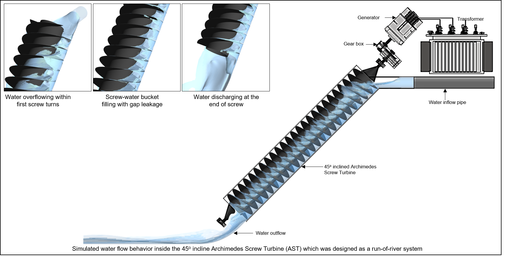
It is convenient to categorize the fluid flow behavior of AST as entrance, middle and exit of the screw domain as shown in
Figure 10.
Figure 10b illustrates the overflowing water phenomena over the screw blade at the screw inlet. The water flow inside the first few screws is turbulent because of the high incoming water velocity and the higher inclination of the screw. When the incoming flow has considerably high speed, the water hits on the screw blade and splash, resulting in an overflow. Since the overflow leakage is a hydro loss, it can be minimized by reducing the incoming velocity with the help of an upper reservoir.
Water is filled into the screw with an optimum filling rate at the optimum rotational speed without forming a reservoir, but at a higher screw speed, the water filling rate is less than the optimum screw filling rate, and hence, a tiny reservoir at the screw inlet is formed.
After passing through the first few screw turns, the water flow becomes steady, filling in each turn, resulting in almost the same pressure force on the blade surfaces. Thus, it is important to understand the difference in water level inside the screw.
Figure 11 illustrates the theoretical [
2] and simulated water filling inside one screw turn. In
Figure 11, points 1,2 and 3,4 are related to the upper water level margins (just before the blade surface, which belongs to the upper screw turn), and points 5 and 6 are related to the down water level margins (just after the blade surface, which belongs to the lower screw turn). This difference in water level exerts the pressure force on the screw blade. The variation in water level is quite similar to the theoretical optimal water level, except for point 4 denoted in
Figure 11b. That is because of the viscosity effect of the water, where the water particles drag up with the blade surface, especially at the blade tip, which has a high tangential velocity. These particular observations are significant in determining the optimum water filling phenomena without overflowing or underfilling conditions [
2,
3]. At lower rotational speeds, water overflowing upon the screw shaft can be observed because of the high filling rate [
21]. At higher rotational speeds, partially filled screw buckets can be observed because of underfilling rates. In comparison, optimum water filling can be observed when the screw rotates at optimal speed.
Figure 12 depicts these phenomena showing the difference between every three scenarios.
As shown in
Figure 13, the highest-pressure difference occurs at the last screw of the turbine since there is no water back-pressure acting on the last blade. Further, as shown in
Figure 10c, water gradually unloads from the screw with lesser turbulence than the screw filling at inlet. Thus,
Figure 13 showed this pressure variation inside the screw which is measured along the line drawn at the screw gap as illustrated in the same figure, when the screw rotates at optimum value.
Except for the inlet and the outlet of the screw, the pressure variation has almost the same peak-trend [
22] inside the screw turn. The pressure difference resulting from the difference in the water level between two nearby screw turns is the key to generating torque on the screw blades. At optimal rotational speed, this pressure difference is estimated as 1800 Pa, as shown in
Figure 13. A zoomed view of the pressure variation clearly shows how the pressure gradually increases and suddenly drops due to the water level difference at the two sides of the screw blades.
Equation (9) explains the difference in water level as a function of the inclination angle, screw pitch, and the number of screws [
7]. Accordingly, a high inclined screw generates a greater pressure difference on the blade due to the considerable water level difference between each screw turn:
According to Equation (9), the difference between the two successive water levels increases by reducing the screw pitch and increasing the screw inclination for a given number of screw turns. When the water level difference is higher, the gap leakage loss due to increased pressure at the bottom of the bucket is also got increased. Therefore, maintaining a minimum possible gap between the screw tip and the trough is essential when designing higher inclined ASTs.
Figure 14 illustrates the velocity contour on the mid-plane of the screw with the axial (along the screw longitudinal direction) and circumferential velocity (along the tangential direction) variation along the screw gap when the screw rotates at 54.58 rpm. Peak axial velocity variation can be observed at the gap between the blade tip and the trough, indicating the gap leakage flow where the velocity direction is longitudinal. There, the water pressure of the upper bucket pushes the water to the lower bucket through the gap. Average axial velocity was estimated as 2 m/s for optimum rotational speed, recording an overall gap leakage flow rate of about 15% from the total flow rate. Further, a low leakage flow was identified for higher rotational speeds due to the low water filling rate at the screw inlet resulting in underfilling conditions. In contrast, the leakage flow is high at low and optimum rotational speeds due to high filling rates even with overflowing conditions. However, it is considered that the leakage loss increases with the increase of inclination angle of AST for all filling conditions. Therefore, it is important to maintain very low gaps in high inclination AST designs to achieve reasonable performance.
5. Conclusions
Most of the AST designs were conducted for low inclination angles since the claimed performance has above 80% efficiency [
7,
23]. The key reasons for these phenomena are that low inclination ASTs can hold the maximum water volume per bucket, creating significant water level differences and lower gap leakage losses, but in the case of a considerably high hydraulic head, low inclination AST results in longer screws affected by bending problems and bearing limitations [
7]. Therefore, this study was conducted to investigate the performance and analyze the flow field with the aspect of pressure and velocity inside the maximum possible inclination AST.
The findings of this study reveal that even for high hydro heads, the highest possible inclination ASTs can be achievable, reaching 80% efficiency. Such performance could be attained by maintaining the maximum water volume per bucket by increasing the number of screw turns (decreasing the screw pitch) and maintaining a minimal possible gap between the blade tip and the screw trough. Thus, a high inclination AST results in a relatively shorter screw relaxing the bending and bearing limitations.
The Rorres’s approach is used in this design also since there is no design procedure for ASTs even though Rorres’s ratios are optimized for Archimedes screw pumps. In Rorres’s study, the optimization is based on lifting the maximum water volume. In contrast, the AST performance depends on the water pressure exerted due to the water volume inside the screw turns. Maximum possible water volume in each screw turns results in the highest pressure on the blades. Thus, designing a completely new AST is more suitable for high inclined situations than trying with AST models already designed for low inclinations. That is because the optimum screw pitch highly depends on the inclination of the AST.
Additionally, ASTs can be designed as a run-of-the-river systems where there is an almost constant flow rate during the operating period. Otherwise, an upper storage reservoir is recommended to have an optimum flow rate into the AST without disturbances. Furthermore, the lower reservoir could be omitted considering the construction cost, available space, design conditions, and environmental conditions. However, the lower reservoir is recommended whenever possible to reach the maximum performance of the AST.
CFD analysis is a valuable tool for analyzing the flow field, especially when the flow behavior becomes complex and also expensive to make experimental studies. Pressure and velocity fields observed by CFD are helpful to identify the internal flow field, such information is useful for further development of AST technology. Furthermore, CFD techniques can be used to simulate the flow field in a real-scale model with real-state information rather than simulating small-scale models to avoid scaling effects.


