Machine Learning-Based Small Hydropower Potential Prediction under Climate Change

Abstract

As the effects of climate change are becoming severe, countries need to substantially reduce carbon emissions. Small hydropower (SHP) can be a useful renewable energy source with a high energy density for the reduction of carbon emission. Therefore, it is necessary to revitalize the development of SHP to expand the use of renewable energy. To efficiently plan and utilize this energy source, there is a need to assess the future SHP potential based on an accurate runoff prediction. In this study, the future SHP potential was predicted using a climate change scenario and an artificial neural network model. The runoff was simulated accurately, and the applicability of an artificial neural network to the runoff prediction was confirmed. The results showed that the total amount of SHP potential in the future will generally a decrease compared to the past. This result is applicable as base data for planning future energy supplies and carbon emission reductions.

1. Introduction

Hydropower is an important renewable energy source. It contributes to sustainability by producing electricity with almost zero greenhouse gas (GHG) emissions [1,2]. In particular, small hydropower (SHP) has the additional advantage of quickly responding to short-term changes in the electricity demand in small-scale areas [3,4,5]. There have been many studies regarding its positive and negative impacts (e.g., ecological impacts on the fluvial ecosystem), as well as the method for mitigating those negative impacts (e.g., environmental flows) [1,2]. In particular, as it is considered to play a key role in mitigating climate change, it has been actively promoted globally. Many studies have been conducted to estimate the SHP potential, and accurately assessing the future potential of SHP is a major concern [6,7,8,9,10,11,12,13,14,15,16,17,18,19].

SHP plants highly depend on climatic conditions; thus, it is crucial to accurately predict the runoff under various climate change scenarios in order to assess the future SHP potential [9,20]. In previous studies, a runoff was simulated using various hydrological models to evaluate the impacts of climate change on the hydropower potential [9,21,22,23,24,25]. For conceptual and lumped models, Kim et al. (2012) predicted the future runoff using the Tank model [26], and Chilkoti et al. (2017) used a conceptual rainfall-runoff model [9]. Depending on the scale and available information of the target area, the hydrological models that can be used may vary [8]. By incorporating data such as the basin slope, curve number, soil database, and digital elevation model (DEM), a more detailed model can be applied. Liu et al. (2016) applied eight global hydrological models to project the impact of climate change on the hydropower potential in China [27]. Kim et al. (2018) and Wang et al. (2019) used a grid-based surface runoff model and variable infiltration capacity model to study the impact of climate change on the future runoff and SHP potential [6,28]. Van Vliet et al. (2016) pointed out the limitations of previous studies that used only one hydrological model and then used an ensemble of results from three global hydrological models [8]. However, the greater the input data used, the greater is the uncertainty of the model [8].

To this end, an artificial neural network (ANN), which is a machine learning model, can be an alternative solution that can overcome the shortcomings of hydrological models. An ANN model is based on the structure of neurons while taking into account nonlinearity and shows highly accurate results in complex systems with less impact from outliers. Because of these strengths, ANNs have been widely used in hydrological and environmental models to study complex nonlinear processes such as the rainfall-runoff process. In particular, ANN has been applied to a wide variety of data and other models in order to calculate and predict flood discharge. Campolo et al. (2003) used three different input data (daily precipitation, hydrometric, and dam operation plan data) into an ANN model to calculate the flood discharge, and they showed better results than regression models [29]. Kerh and Lee (2006) developed an ANN model based on upper stream station data and basin characteristics to predict the characteristics of the lower stream stations, and the developed model yielded more accurate results than those from the Muskingum method [30]. Nesliihan (2011) predicted 543 ungauged basins in Turkey using two types of ANNs, and Hidayat et al. (2014) applied ANN to tidal rivers and showed that ANN could perform accurate predictions with less target station water level data [31,32]. Jahangir et al. (2019) added Geographic Information System (GIS) data to an ANN model, and Bomers et al. (2019) used a 1-D/2-D coupled hydraulic model to teach an ANN model to reproduce past 1809 flood events. Both studies recognized that their ANN model performed better than existing models [33,34]. As such, research on predicting the future runoff by using an ANN model has been conducted; however, there has been no research that has used the runoff predicted by the ANN model to estimate the SHP potential.

Therefore, this study applied the ANN model to predict the future runoff and then estimated the SHP potential based on the runoff prediction. The target SHP plant and data are described, and the climate change scenario, ANN, evaluation metrics, and SHP potential calculation are explained in Section 2. The results of the future SHP potential prediction are presented in Section 3. The conclusions are presented in Section 4.

2. Data Descriptions and Methods

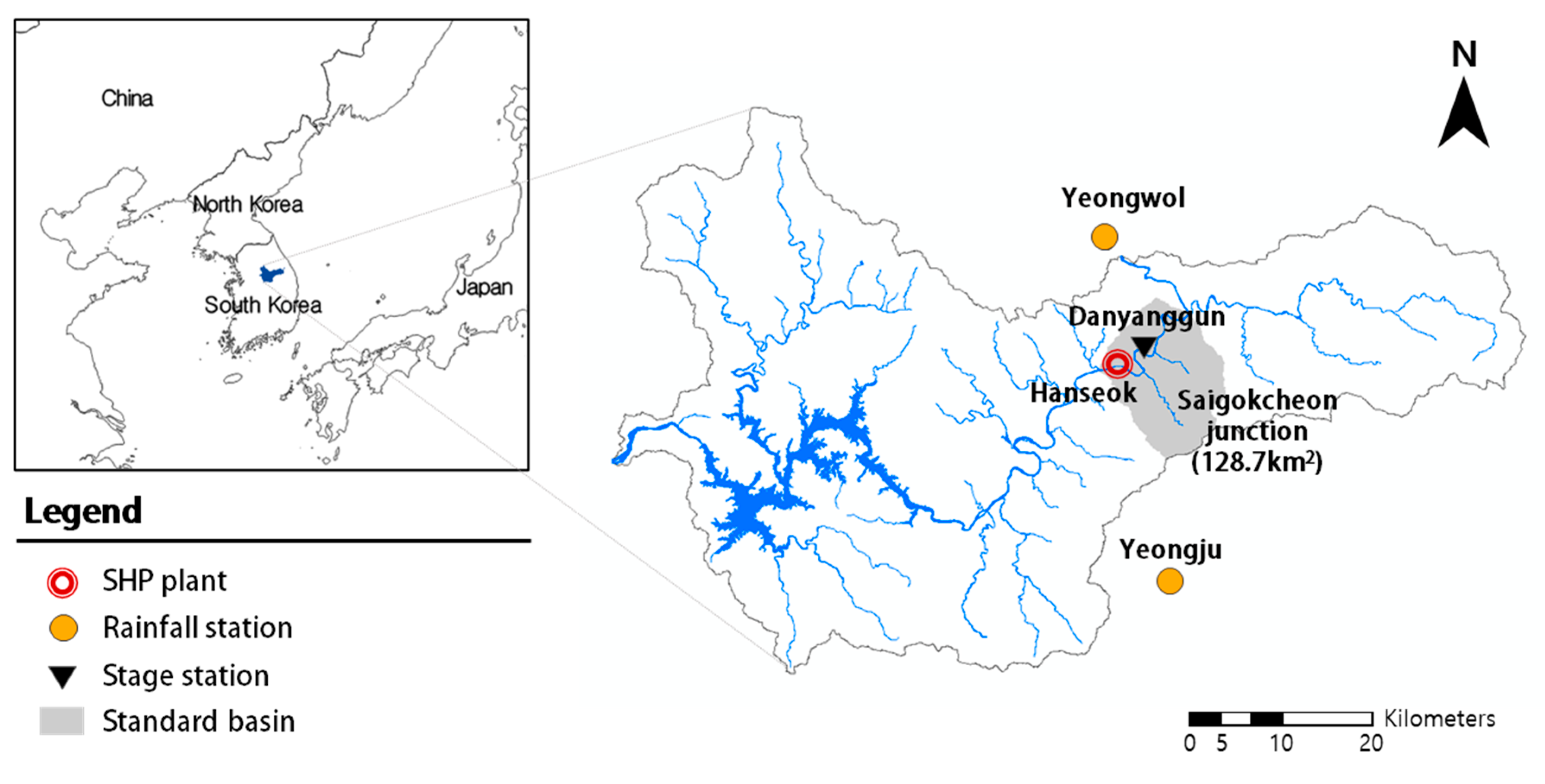
2.1. Target SHP Plant and Data

In this study, the Hanseok power plant in the Han River basin of South Korea was selected as the target plant. As of 2015, there were 61 SHP plants currently in operation in South Korea. The target plant was selected based on the following criteria: (1) the existence of a rainfall station and a stage station with available weather and discharge data, (2) the existence of over 2000 kW of power plant capacity that guarantees a stable power plant operation, and (3) the possession of power generation data for 10 years or longer. In particular, for the application of ANN, the training period should be at least two times longer than the test period, and the available observed data was an important criterion for this selection.

The Hanseok SHP plant is in the standard basin of the Saigokcheon junction. There are two rainfall stations (Yeongwol and Yeongju) and a stage station (Danyanggun) in operation near the plant (Figure 1). It has been generating electricity since its construction in 1989, with an installed capacity of 2214 kW and an effective head of 3.8 m.

Weather data were collected from two nearby rainfall stations. These two stations, Yeongwol and Yeongju, are under the control of the Korea Meteorological Administration (KMA). The daily observed data for the precipitation, average temperature, average wind speed, and average relative humidity for the period of 1995 to 2020 were collected. The daily average discharge data for the same period were collected from the Danyanggun stage station.

2.2. Climate Change Scenario

A climate change scenario can be defined as the future carbon dioxide concentration in the atmosphere to be used as the forced condition of a climate change model. The Intergovernmental Panel on Climate Change (IPCC) has been developing future climate change scenarios based on GHG emission scenarios and evaluating climate change response strategies. In the IPCC fifth assessment report in 2014 (AR5), GHG concentrations were determined based on the radiation to the atmosphere caused by human activities. Representative Concentration Pathways (RCPs) were developed to indicate that socio-economic scenarios may vary for one representative radiative forcing. The RCP scenarios consist of four different cases (2.6, 4.5, 6.0, and 8.5) according to climate change response policies (

Table 1. Brief explanation of the RCP scenarios (2.6,4.5,6.0, and 8.5).

RCP	Case	$\mathbf{C}{\mathbf{O}}_2\mathbf{Concentration}$
2.6	The Earth is able to recover the effects of human activities (Impossible Scenario)	420 ppm
4.5	The green gas reduction policies are implemented significantly	540 ppm
6.0	The green gas reduction policies are realized at less than RCP 4.5	670 ppm
8.5	The greenhouse gases are emitted at the current trend (without reduction)	940 ppm

).

RCP scenarios are materialized through global climate models (GCMs) and are used as the most general climate change forecast data. GCMs are global atmosphere-ocean circulation models based on complex interactions among various forces, such as solar radiation energy, volcanic eruptions, greenhouse effect, and various other conditions including the atmosphere, oceans, and ground surface. However, it is difficult to use GCMs to analyze regional areas because of their low resolution (135 × 135 km). Therefore, a spatial and temporal downscaling must be conducted to use a GCM at a regional scale.

To simulate the future climate of South Korea, the KMA is preparing a global climate change scenario using the Coupled Model Intercomparison Project phase 5 (CMIP5). Among several CMIP5 models, the GCM of Hadley Center Global Environment Model-Regional Climate Model (HadGEM3-RA) from the Hadley Center (UK Met Office) is widely used to understand climate change and provide future climate projections [35,36]. As aforementioned, it is difficult to use a GCM for South Korea. Therefore, the KMA uses HadGEM3-RA, a regional climate model from HadGEM2-AO, for East Asia and the Korean Peninsula. However, the regional climate model is still large for studying small areas such as watersheds. Thus, the KMA offers fine-scale (1 × 1 km) climate change data over South Korea. To prepare the fine-scale data, the KMA used the Parameter-elevation Regression on Independent Slopes Model (MK-PRISM) and PRSIM-based Downscaling Estimation Model (PRIDE) to downscale the HadGEM3-RA. This study used fine-scale data from the KMA as future climate data.

We collected daily RCP 4.5 scenarios containing the precipitation, average temperature, relative humidity, and average wind speed from 2021 to 2030. RCP 4.5 is mainly used to estimate the long-term runoff and considers the substantial realization of GHG reduction policies [37]. Because of the underestimation of precipitation data in the climate change scenario, outlier testing and bias correction through quantile mapping are required [38]. Therefore, this study used quantile mapping for the bias correction and the box plot method to detect outliers. After applying the two methods, we calculated the basin average value of each meteorological factor in the observation data and climate change scenario data by assigning the Thiessen polygon area ratio.

2.3. Artificial Neural Network

The ANN model, introduced by McCulloch and Pitts (1943), is a representative supervised machine-learning algorithm [39]. The ANN model is based on the human brain system and is generally used for the classification and prediction of specific factors using only undefined mathematical relationships. The model is known to be an effective method for analyzing nonlinear relationships between independent and dependent variables in given datasets. Figure 2 illustrates the conceptual diagram of the ANN model.

The ANN model consists of three layers, namely the input, hidden, and output layers (Figure 2), each of which possesses a set of neurons that are fully connected with neurons in the following layer, and each layer has different weight values (w). The ANN model aims to reduce errors, defined as the difference between the estimated and targeted values, by modifying the weights using the backward propagation process. The backward propagation process involves adjusting the parameters (e.g., weights, w, and biases, b) of the model based on the loss provided from the previous iteration. Proper tuning results ensure minimum errors, making the model reliable by increasing its generalization. The ANN model was mathematically formulated using Equation (1):

$$\begin{gathered} {\mathrm{f}}_1=f\left(b_1+w_{11}{\mathrm{X}}_1+w_{21}{\mathrm{X}}_2+\cdots +w_{n1}{\mathrm{X}}_n\right) \\ {\mathrm{f}}_2=f\left(b_2+w_{12}{\mathrm{X}}_1+w_{22}{\mathrm{X}}_2+\cdots +w_{n2}{\mathrm{X}}_n\right) \\ ⋮ \\ {\mathrm{f}}_m=f\left(b_m+w_{1m}{\mathrm{X}}_1+w_{2m}{\mathrm{X}}_2+\cdots +w_{nm}{\mathrm{X}}_n\right) \\ Y=f\left(B_0+W_{10}{f}_1+W_{20}{f}_2+\cdots +W_{m0}{f}_m\right) \end{gathered}$$

(1)

where X is an input variable, f denotes an activation function for the layers, w represents the weight values between layers, and b and B indicate the biases in the hidden and output layers, respectively. In the algorithms of the ANN model, the input X is multiplied by the weight value, and the coupled value is then converted by the activation function. Subsequently, it is transmitted to the next layer as a signal. Through these processes, the final output Y is obtained. The representative activation functions generally used in the ANN model include the sigmoid, hyperbolic tangent (tanh), and rectified linear unit (Relu) functions.

2.4. Evaluation Metrics

In this study, the three metrics used for evaluating the performance of the ANN model for runoff forecasting were the Nash–Sutcliffe efficiency (NSE), coefficient of coefficient (CC), and percent bias (PBIAS).

$$\mathrm{NSE}=1-\frac{{\displaystyle \sum }{\left(y_e-y_o\right)}^2}{{\displaystyle \sum }{\left(y_o-\overline{y_o}\right)}^2}$$

(2)

$$\mathrm{CC}=\frac{{\displaystyle \sum }\left(y_e-\overline{y_e}\right)\left(y_o-\overline{y_o}\right)}{{\displaystyle \sum }\left(y_e-\overline{y_e}\right){\displaystyle \sum }\left(y_o-\overline{y_o}\right)}$$

(3)

$$\mathrm{PBIAS}=\frac{{\displaystyle \sum }{y}_o-{\displaystyle \sum }{y}_e}{{\displaystyle \sum }{y}_o}\times 100 (\%)$$

(4)

where y_e and y_o denote the simulated and observed runoff, respectively, and $\overline{y_e}$ and $\overline{y_o}$ are the average values of the simulated and observed runoff, respectively. The CC ranges from −1 to 1 and describes a measure of how well the outputs are simulated by the model. A value of 0 indicates that there was no correlation between the two runoff datasets. The PBIAS indicates the ratio of the difference between the sum of simulated and observed runoffs to the sum of the observed runoff. It is generally used to evaluate the modeling performance of runoff volumes. The NSE denotes the predictive power of the model. It ranges from −∞ to 1, and a value closer to 1 indicates a better performance of the model, while a value below zero indicates that the average observed value is better than the modeled value.

2.5. SHP Potential Calculation

The theoretical potential of SHP is the energy that can be obtained without considering the geographical and technical constraints. The theoretical potential was calculated as follows:

$$P_t=\rho ·g·Q·H\left(\mathrm{kW}\right)$$

(5)

where the water density is $\rho$ (kg/m³), the runoff is Q (${\mathrm{m}}^3/\mathrm{s}$), the head is H (m), and g is the acceleration due to gravity ($\mathrm{m}/{\mathrm{s}}^2)$. The density of water was taken as 1000 kg/m³, and the acceleration due to gravity was approximately 9.8$\mathrm{m}/{\mathrm{s}}^2$. The effective head ($H_e$), the height of the head, which determines the energy, was used as the head. The value of H can be obtained by excluding loss head (head loss) from the gross head. The designed discharge ($Q_d$ (${\mathrm{m}}^3/\mathrm{s})$) value was applied. In this study, the maximum power generation potential of the Hanseok SHP plant was taken as 53 MW, and the maximum runoff contributing to power generation was 158.3${\mathrm{m}}^3/\mathrm{s}$. Therefore, we calculated the potential by applying 158.3${\mathrm{m}}^3/\mathrm{s}$ as the design discharge.

The technical potential can be calculated from the theoretical potential by considering the efficiency of the plant (η) and the operation rate ($L_f)$. The technical potential was calculated as follows:

$$\mathrm{P} = \rho ·g·Q_d·H_e·\eta ·L_f \left(\mathrm{kW}\right)$$

(6)

The total efficiency (η) varies according to the size and type of the plant. In this study, the efficiency and operation rate were assumed to be 0.8 and 0.4, respectively [40].

3. Results

3.1. ANN Model Development

The ANN model used in this study had a standard three-layer network. It consisted of an input layer, hidden layer, and output layer, and included a Relu activation function in the hidden layer and a linear transfer function in the output layer. This study examined the runoff prediction performance using various numbers of hidden layers, and the results showed the most reliable results when using two hidden layers. The simulation function of the algorithms for predicting the runoff was as follows:

$$Q_{t+m}=f\left(P_{t-n},H_{t-n},T_{t-n},W_{t-n}\right)$$

(7)

where Q_t−m is the predicted runoff with a lead time of m, and P_t−n, H_t−n, T_t−n, and W_t−n indicate antecedent precipitation, humidity, temperature, and wind speed with a previous time step of n, respectively. In this study, the input variables were obtained from two weather stations, and different values of n were considered between one and four days of the previous time steps. A fully connected layer with 40 neurons was used as the input layer. In this study, for the runoff prediction using the ANN model, the training period was from January 1995 to December 2015, the validation period was from January 2016 to December 2020, and the test period was from January 2021 to December 2030.

3.2. Runoff Prediction under A Climate Change Scenario Using ANN Model

The trained ANN model was used for the verification and testing of runoff predictions. Figure 3 illustrates the validation results for the runoff prediction using the ANN model from January 2016 to December 2020. As shown in the figure, the model could accurately capture the variability of the runoff in time and peak runoff. Statistical metrics showed the predictive performance of the model. The values of CC, PBIAS, and NSE were 0.77, 16.8%, and 0.6, respectively. According to Moriasi et al. (2007) and Xiang et al. (2020), in hydrologic modeling, an NSE value over 0.5 is considered acceptable, indicating that the ANN model used in this study provided a sufficient predictive performance in forecasting the runoff [41,42].

3.3. SHP Potential Prediction

The future SHP potential (2021–2030) was predicted using future runoff simulation results. The results of the monthly SHP potential are shown in Figure 4. In the prediction period of 2021–2030, the SHP potential decreased as compared to that of the historic period. This result can be attributed to a decrease in precipitation in future climate change scenarios. The decreasing trend of precipitation in the 2020s has also been mentioned in previous studies [43,44,45].

Table 2. The statistics of the monthly SHP potential in the historic and future periods.

Statistic	Historic (2000–2020)	Future (2021–2030)	Change (%)
Max.	1581.69	855.63	−45.9%
75%	657.02	467.93	−28.8%
50%	371.07	328.09	−11.6%
25%	201.55	235.51	16.9%
Min.	9.41	78.55	734.6%
Mean	491.79	364.20	−25.9%

shows the comparison between the statistics of the monthly SHP potential in the historic and future prediction periods. The maximum to mean value of the SHP potential in the future period indicates a lower value than the values in the historic period, with a change of −45.9% to −11.6%. On the other hand, the lower quartile (25%) and minimum values showed an increase in the future period, with a change of 16.9% to 734.6%. The monthly average potentials of each period are compared in Figure 5. Overall, the average monthly potential decreased in the future period as compared to that of the historic period, particularly from July to September. However, future increases in the monthly average potential showed the largest change in June, with 59%. These results indicate that the variation in the SHP potential will decrease in the future, similar to the characteristics of precipitation in the climate change scenarios.

4. Conclusions and Discussion

Efforts for achieving carbon neutrality are needed in order to mitigate global climate crises. To this end, it is necessary to develop eco-friendly sources of energy and SHP. In this study, we attempted to accurately predict the future SHP potential using a climate change scenario and an ANN model. The Hanseok SHP plant was selected as the target plant. The future runoff was simulated using the ANN model while considering climate change, and the future SHP potential was subsequently predicted. The runoff simulation results of the ANN model showed a sufficient predictive performance with a CC value of 0.77, PBIAS of 16.8%, and NSE of 0.6. The results showed that the model accurately captured the variability and peak runoff. The future SHP potential was predicted using the future runoff. The results indicate that the SHP potential will decrease from 2021 to 2030. In particular, the maximum value of the monthly SHP potential in the future period was predicted to decrease by 45.9% compared to that in the historic period. In addition, the results of monthly average potentials showed that the average potential during July to September was expected to decrease, while an opposite trend was shown in June.

This study contributes to improving the predictive performance of the future SHP potential by using an ANN model. Though this study was conducted for a target SHP plant, it can also be applied to any SHP plant. Owing to this limitation, we assumed the most conservative value for the analysis, as the accurate operation rate and design discharge of the plant were not available. In actual applications, more accurate predictions are possible using more accurate values. In addition, machine learning models including ANN have limitations that learn from observation data and make a prediction based on them, so that the model is highly dependent on the learning data. Even if the length of the training period is long enough and the characteristics of the selected training data can represent the characteristics of the whole data, it is difficult to predict future extreme events that have not occurred in the past. It is possible to make more accurate predictions by taking these limitations into account and finding ways to complement those of existing models based on the results of the models used in this study; it is then expected that this study can be used to plan for future energy supplies and carbon emission reductions.

References

1. Kuriqi, A.; Pinheiro, A.N.; Sordo-Ward, A.; Garrote, L. Water-energy-ecosystem nexus: Balancing competing interests at a run-of-river hydropower plant coupling a hydrologic–ecohydraulic approach. Energy Convers. Manag. 2020, 223, 113267. [Google Scholar] [CrossRef]
2. Kuriqi, A.; Pinheiro, A.N.; Sordo-Ward, A.; Bejarano, M.D.; Garrote, L. Ecological impacts of run-of-river hydropower plants—Current status and future prospects on the brink of energy transition. Renew. Sustain. Energy Rev. 2021, 142, 110833. [Google Scholar] [CrossRef]
3. Frey, G.W.; Linke, D.M. Hydropower as a renewable and sustainable energy resource meeting global energy challenges in a reasonable way. Energy Policy 2002, 30, 1261–1265. [Google Scholar] [CrossRef]
4. Llamosas, C.; Sovacool, B.K. The future of hydropower? A systematic review of the drivers, benefits and governance dynamics of transboundary dams. Renew. Sustain. Energy Rev. 2021, 137, 110495. [Google Scholar] [CrossRef]
5. Francisco, M.A.; Myriam, T.; Antonio, Z.S.; Adel, J.; Francisco, G.M. An overview of research and energy evolution for small hydropower in Europe. Renew. Sustain. Energy Rev. 2017, 75, 476–489. [Google Scholar]
6. Freitas, M.A.V.; Soito, J.L.S. Vulnerability to climate change and water management: Hydropower generation in Brazil. WIT Trans. Ecol. Environ. 2009, 124, 217–228. [Google Scholar] [CrossRef] [Green Version]
7. Hamududu, B.; Killingtveit, A. Assessing Climate Change Impacts on Global Hydropower. Energies 2012, 5, 305–322. [Google Scholar] [CrossRef] [Green Version]
8. Van Vliet, M.; van Beek, L.; Eisner, S.; Flörke, M.; Wada, Y.; Bierkens, M. Multi-model assessment of global hydropower and cooling water discharge potential under climate change. Glob. Environ. Chang. 2016, 40, 156–170. [Google Scholar] [CrossRef]
9. Chilkoti, V.; Bolisetti, T.; Balachandar, R. Climate change impact assessment on hydropower generation using multi-model climate ensemble. Renew. Energy 2017, 109, 510–517. [Google Scholar] [CrossRef]
10. Fan, J.-L.; Hu, J.-W.; Zhang, X.; Kong, L.-S.; Li, F.; Mi, Z. Impacts of climate change on hydropower generation in China. Math. Comput. Simul. 2020, 167, 4–18. [Google Scholar] [CrossRef]
11. Kumar, A.; Schei, T.; Ahenkorah, A.; Rodriguez, R.; Devernay, J.; Freitas, M.; Hall, D.; Killingtveit, Å.; Liu, Z.; Edenhofer, O.; et al. (Eds.) IPCC Special Report on Renewable Energy Sources and Climate Change Mitigation; Cambridge University Press: Cambridge, UK; New York, NY, USA, 2011. [Google Scholar]
12. Markoff, M.S.; Cullen, A.C. Impact of climate change on Pacific Northwest hydropower. Clim. Chang. 2007, 87, 451–469. [Google Scholar] [CrossRef]
13. Minville, M.; Brissette, F.; Krau, S.; Leconte, R. Adaptation to Climate Change in the Management of a Canadian Water-Resources System Exploited for Hydropower. Water Resour. Manag. 2009, 23, 2965–2986. [Google Scholar] [CrossRef]
14. Vicuna, S.; Leonardson, R.; Hanemann, M.W.; Dale, L.L.; Dracup, J.A. Climate change impacts on high elevation hydropower generation in California’s Sierra Nevada: A case study in the Upper American River. Clim. Chang. 2007, 87, 123–137. [Google Scholar] [CrossRef]
15. Vicuña, S.; Dracup, J.A.; Lund, J.R.; Dale, L.L.; Maurer, E.P. Basin-scale water system operations with uncertain future climate conditions: Methodology and case studies. Water Resour. Res. 2010, 46. [Google Scholar] [CrossRef] [Green Version]
16. Raje, D.; Mujumdar, P. Reservoir performance under uncertainty in hydrologic impacts of climate change. Adv. Water Resour. 2010, 33, 312–326. [Google Scholar] [CrossRef]
17. Koch, F.; Prasch, M.; Bach, H.; Mauser, W.; Appel, F.; Weber, M. How Will Hydroelectric Power Generation Develop under Climate Change Scenarios? A Case Study in the Upper Danube Basin. Energies 2011, 4, 1508–1541. [Google Scholar] [CrossRef]
18. Schaefli, B.; Hingray, B.; Musy, A. Climate change and hydropower production in the Swiss Alps: Quantification of potential impacts and related modelling uncertainties. Hydrol. Earth Syst. Sci. 2007, 11, 1191–1205. [Google Scholar] [CrossRef]
19. Majone, B.; Villa, F.; Deidda, R.; Bellin, A. Impact of climate change and water use policies on hydropower potential in the south-eastern Alpine region. Sci. Total. Environ. 2016, 543, 965–980. [Google Scholar] [CrossRef]
20. Schaefli, B. Projecting hydropower production under future climates: A guide for decision-makers and modelers to interpret and design climate change impact assessments. Wiley Interdiscip. Rev. Water 2015, 2, 271–289. [Google Scholar] [CrossRef] [Green Version]
21. Arriagada, P.; Dieppois, B.; Sidibe, M.; Link, O. Impacts of Climate Change and Climate Variability on Hydropower Potential in Data-Scarce Regions Subjected to Multi-Decadal Variability. Energies 2019, 12, 2747. [Google Scholar] [CrossRef] [Green Version]
22. Carvajal, P.E.; Anandarajah, G.; Mulugetta, Y.; Dessens, O. Assessing uncertainty of climate change impacts on long-term hydropower generation using the CMIP5 ensemble—the case of Ecuador. Clim. Chang. 2017, 144, 611–624. [Google Scholar] [CrossRef] [Green Version]
23. Eshchanov, B.; Abylkasymova, A.; Overland, I.; Moldokanov, D.; Aminjonov, F.; Vakulchuk, R. Hydropower Potential of the Central Asian Countries. Cent. Asia Reg. Data Rev. 2019, 19, 1–7. [Google Scholar]
24. Hu, Y.; Jin, X.; Guo, Y. Big data analysis for the hydropower development potential of ASEAN-8 based on the hydropower digital planning model. J. Renew. Sustain. Energy 2018, 10, 034502. [Google Scholar] [CrossRef]
25. Hamududu, B.H.; Killingtveit, Å. Hydropower Production in Future Climate Scenarios; the Case for the Zambezi River. Energies 2016, 9, 502. [Google Scholar] [CrossRef] [Green Version]
26. Kim, G.J.; Sun, S.P.; Yeo, G.D.; Kim, H.S. A Study on Variability of Small Hydro Power Generation Considering Climate change. KSCE Conv. Korean Soc. Civ. Eng. 2012, 10, 932–935. [Google Scholar]
27. Liu, X.; Tang, Q.; Voisin, N.; Cui, H. Projected impacts of climate change on hydropower potential in China. Hydrol. Earth Syst. Sci. 2016, 20, 3343–3359. [Google Scholar] [CrossRef] [Green Version]
28. Wang, H.; Xiao, W.; Wang, Y.; Zhao, Y.; Lu, F.; Yang, M.; Hou, B.; Yang, H. Assessment of the impact of climate change on hydropower potential in the Nanliujiang River basin of China. Energy 2019, 167, 950–959. [Google Scholar] [CrossRef]
29. Campolo, M.; Soldati, A.; Andreussi, P. Artificial neural network approach to flood forecasting in the River Arno. Hydrol. Sci. J. 2003, 48, 381–398. [Google Scholar] [CrossRef]
30. Kerh, T.; Lee, C. Neural networks forecasting of flood discharge at an unmeasured station using river upstream information. Adv. Eng. Softw. 2006, 37, 533–543. [Google Scholar] [CrossRef]
31. Neslihan, S. Modeling flood discharge at ungauged sites across Turkey using neuro-fuzzy and neural networks. J. Hydroinform. 2011, 13, 842–849. [Google Scholar]
32. Hidayat, H.; Hoitink, A.J.F.; Sassi, M.G.; Torfs, P.J.J.F. Prediction of Discharge in a Tidal River Using Artificial Neural Networks. J. Hydrol. Eng. 2014, 19, 04014006. [Google Scholar] [CrossRef]
33. Jahangir, M.H.; Reineh, S.M.M.; Abolghasemi, M. Spatial predication of flood zonation mapping in Kan River Basin, Iran, using artificial neural network algorithm. Weather. Clim. Extrem. 2019, 25, 100215. [Google Scholar] [CrossRef]
34. Bomers, A.; van der Meulen, B.; Schielen, R.M.J.; Hulscher, S.J.M.H. Historic Flood Reconstruction With the Use of an Artificial Neural Network. Water Resour. Res. 2019, 55, 9673–9688. [Google Scholar] [CrossRef] [Green Version]
35. Kyoung, M.; Kim, H.S.; Sivakumar, B.; Singh, V.; Ahn, K. Dynamic characteristics of monthly in the Korean Peninsular under climate change. Stoch. Environ. Res. Risk Assess. 2011, 25, 613–625. [Google Scholar] [CrossRef]
36. Bodas-Salcedo, A.; Mulcahy, J.P.; Andrews, T.; Williams, K.D.; Ringer, M.A.; Field, P.R.; Elsaesser, G.S. Strong Dependence of Atmospheric Feedbacks on Mixed-Phase Microphysics and Aerosol-Cloud Interactions in HadGEM3. J. Adv. Model. Earth Syst. 2019, 11, 1735–1758. [Google Scholar] [CrossRef] [PubMed] [Green Version]
37. Kim, J.W. Prediction and Evaluation of Hydro-Ecology, Functions, and Sustainability of a Wetland under Climate Change. Ph.D. Thesis, Inha University, Incheon, Korea, 2019. [Google Scholar]
38. Kwak, J.; Kim, S.; Jung, J.; Singh, V.P.; Lee, N.R.; Kim, H.S. Assessment of Meteorological Drought in Korea under Climate Change. Adv. Meteorol. 2016, 2016, 1–13. [Google Scholar] [CrossRef]
39. McCulloch, W.S.; Pitts, W. A logical calculus of the ideas immanent in nervous activity. Bull. Math. Biol. 1943, 5, 115–133. [Google Scholar] [CrossRef]
40. Jung, S. Estimation and Future Prospect of Small Hydropower Generation Potential for the Ungaged Basin. Ph.D. Thesis, Inha University, Incheon, Korea, 2020. [Google Scholar]
41. Moriasi, D.N.; Arnold, J.G.; Van Liew, M.W.; Bingner, R.L.; Harmel, R.D.; Veith, T.L. Model Evaluation Guidelines for Systematic Quantification of Accuracy in Watershed Simulations. Trans. ASABE 2007, 50, 885–900. [Google Scholar] [CrossRef]
42. Xiang, Z.; Yan, J.; Demir, I. A rainfall-runoff model with LSTM-based sequence-to-sequence learning. Water Resour. Res. 2020, 56, e2019WR025326. [Google Scholar] [CrossRef]
43. Andrade, C.W.L.; Montenegro, S.M.G.L.; Montenegro, A.A.A.; Lima, J.R.D.S.; Srinivasan, R.; Jones, C.A. Climate change impact assessment on water resources under RCP scenarios: A case study in Mundaú River Basin, Northeastern Brazil. Int. J. Clim. 2021, 41, 1045–1061. [Google Scholar] [CrossRef]
44. Tarekegn, N.; Abate, B.; Muluneh, A.; Dile, Y. Modeling the impact of climate change on the hydrology of Andasa watershed. Model. Earth Syst. Environ. 2021, 1–17. [Google Scholar] [CrossRef]
45. Jung, J.; Jung, S.; Lee, J.; Lee, M.; Kim, H. Analysis of Small Hydropower Generation Potential: (2) Future Prospect of the Potential under Climate Change. Energies 2021, 14, 3001. [Google Scholar] [CrossRef]
Figure 1. Location map of the target SHP plant, stations, and basin.
Energies 14 03643 g001
Figure 2. Conceptual diagram of the artificial neural network model.
Energies 14 03643 g002
Figure 3. Validation results of the ANN model using a time-series of the observed and predicted runoff from 2016 to 2020.
Energies 14 03643 g003
Figure 4. Monthly SHP potential in historic and future periods.
Energies 14 03643 g004
Figure 5. Monthly average potentials of the historic and future periods.
Energies 14 03643 g005