Applied Machine Learning Techniques for Performance Analysis in Large Wind Farms

Abstract

As the amount of information collected by wind turbines continues to grow, so too does the potential of its leveraging. The application of machine learning techniques as an advanced analytic tool has proven effective in solving tasks whose inherent complexity can outreach expert-based ability. Such is the case presented by this study, in which the dataset to be leveraged is high-dimensional (79 turbines × 7 SCADA channels) and high-frequency (1 Hz). In this paper, a series of machine learning techniques is applied to the retrospective power performance analysis of a withheld test set containing SCADA data collectively representing 2 full days worth of operation at the Horns Rev I offshore wind farm. A sequential machine-learning based methodology is thoroughly explored, refined, then applied to the power performance analysis task of identifying instances of abnormal behaviour; namely instances of wind turbine under and over-performance. The results of the final analysis suggest that a normal behaviour model (NBM), consisting of a uniquely constructed artificial neural network (ANN) variant trained on abnormality filtered dataset, indeed proves effective in accomplishing the power performance analysis objective. Instances of over and under performance captured by the developed NBM network are presented and discussed, including the operation status of the turbines and the uncertainty embedded in the prediction results.

1. Introduction

The wind energy industry and field of machine learning share a relationship that has spanned decades. Recently, however, this relationship has entered the industry’s innovational main stage as technological advancements have enabled access to unprecedented levels of computational power and information access. Though wind energy has always existed as a data-driven industry, this increasingly facilitated application of machine learning allows for data utilisation on a new scale, one that is actively improving the design, control and analytical insights derived from new and existing wind energy applications.

As the core technologies supporting wind energy (e.g., the design, fabrication and application of the wind turbine and distribution of its power) have reached relatively mature states of general development, a new focus has been placed on the importance of data utilisation in an effort to drive down the levelised cost of energy produced by wind turbines and sold to the electricity market. This utilisation comes in many forms, but perhaps the two most general regimes in the context of machine learning are the forecasting of wind power to improve bids to the electricity market and the monitoring of existing field data in an effort to aid the ongoing operation and maintenance of wind turbines and wind farms at large. The topics addressed by this study concern the latter domain more directly. Within this domain, the main application types are structural health monitoring (SHM), condition monitoring (CM) and performance monitoring (PM).

A fundamental way in which PM differs from SHM and CM is in that its output for a single wind turbine can rely significantly on the the outputs of other wind turbines within the wind farm. Thus, an important application of PM is to identify methodologies that do and do not allow a collection of wind turbines within a wind farm to perform synergistically in an effort to refine control schemes both on a wind turbine and wind farm level. This topic, broadly referred to as wind farm control, has become more prevalent as advanced data analysis has offered increasingly accurate characterisation of the complex aerodynamic interactions within wind farms consisting of many turbines.

This study concerns a novel machine learning-based methodology that can serve the aforementioned goals of PM. In it, historic SCADA data from the Horns Rev I offshore wind farm are used as a basis for development and testing of the proposed methodologies.

The overarching goal of the monitoring tasks, including PM, is to detect system abnormalities, and the general methodology that can be employed to accomplish this goal is referred to collectively as normal behaviour modelling (NBM). In short, the normal behaviour modelling method consists of training a model to understand only normalcy, so that when exposed to new and potentially abnormal observations, low model support of these observations suggests the presence of abnormality. For machine learning models that are typically employed in NBM, the level of a model’s support for an observation can come in different forms based on the model type. In general, support can be a regression model’s prediction error, a density model’s probability assignment or a distance-based method’s calculated relative distances. The general flow of building and applying a NBM with the purpose of monitoring abnormalities can be described by the flow chart presented in Figure 1. The procedures within the NBM flowchart are briefly explained with example implementations in wind energy field below.

Of all the general NBM steps shown in Figure 1, the three most relevant to this work’s methodology are described below.

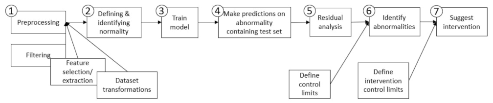
(1)

Preprocessing: The first step in NBM flowchart is preprocessing, which prepares data for both training and testing the NBM. It includes the procedures of filtration (see, e.g., in [1]), feature selection (e.g., recursive feature elimination (RFE) as in [2], tree-based out-of-bag permutation importance matrix (OOB) [3], brute-force sensitivity analysis [4] and feature extraction (FE) [5,6]) and transformation of the dataset (e.g., normalisation, standardisation and case-specific selective transformation [7]). These sub-steps clean the dataset of identifiably faulty data, refine the feature set and scale the data such that the different features’ significance on model performance are comparable. In short, this first step refines the dataset so as to yield a set of features and targets clearly possessing the relationships needed for the modelling task.

(2)

Defining and Identifying Normality: The second step of the NBM flowchart is to choose specific observations which represent system normality to train the NBM. The methods applied for this step vary the most in wind energy applications throughout the literature. For example, the authors of [8] take advantage of a binary label feature in the considered dataset, which indicates wind turbine “healthy” or “unhealthy” status and is tied to the error flags of different system components. In, e.g., [1,9], normal behaviour is defined considering a period after an act of repair or maintenance, assuming it represents the wind turbine operating at its most normal state. In the absence of labelled data or known periods of assumed normalcy, the act of defining normality becomes less trivial. For such a task, various types of machine learning-based outlier detection algorithms can be used to isolate and filter instances of abnormal observations [5,10].

(3)

Train and evaluate model: For the third step in NBM flowchart, two general approaches are typically used: the training of a regression model or of a density model; with the use of the former being far more prevalent than the latter through the literature surveyed. An overview of the machine learning algorithms used for NBM is presented in

Table 1. Selected machine learning algorithms used in NBM.

Model Type	Machine Learning Model	Selected References
Regression	feedforward artificial neural network (ANN-FF)	[4,8,11]
	random forest regression (RFR)	[3,4,12]
	K-nearest neighbours regression (KNNR)	[13,14]
	support vector regression (SVR)	[3,11]
	linear regression (LR)	[9,11]
	Lasso LR	[2]
	Gaussian process (GP)	[8]
	long short-term memory ANN (ANN-LSTM)	[6]
		[7]
	fuzzy inference systems & logic	[13]
Density	Gaussian mixture model (GMM)	[1,10]

. A regression model is trained in order to predict a response variable given explanatory variables. In the case of a regression-based NBM model, if it is trained on a dataset representing purely normal behaviour, then any deviation from a residual of 0 when presented with new test set observations would indicate abnormality.

Herein, the majority of the NBM workflow in Figure 1 is implemented with the exception of defining intervention limits and making intervention suggestions, a step which introduces a temporal aspect to residual-based control limits, e.g., suggesting intervention in the form of repair or replacement of an affected component after its NBM’s residual signal has exceeded its control limit a certain number of times (as in [9]). However, this study differs from the previous studies of NBM applied within the wind energy field (including but not limited to PM) in the chain of methodologies that are applied as well as the utilisation of high-frequency (1 Hz) SCADA data of a large offshore wind farm. Table 1 classifies the methodologies used for NBM with utilisation of SCADA data within the most relevant literature for the study presented here. For CM, the authors of [4,9] investigate a single turbine using 10 min SCADA data, which are then extended to wind farm level in [2,13], respectively. Similarly for PM via 10 min SCADA data, a case study for a single turbine is reported in [1] and wind farm level analyses are performed in [7,8]. With increasing availability of high(er) frequency SCADA signals, the authors of [3,12] investigated the added value of employing 0.25 Hz (4 s) resolution data for PM at wind farms. The authors of [6] utilized 1 Hz SCADA into the workflow with ANN-LSTM networks with the objective of real-time power curve assessment and available power estimation including data-driven wake modelling. Distinctly here in this study, the potential of high-frequency SCADA from Horns Rev-I is fully harnessed to generate a data-driven workflow for PM of large wind farms with state-of-the-art machine learning techniques.

The structure of the paper is as follows. In Section 2 of the investigation presented here, first all available raw SCADA data are processed and assembled into a single dataset for all wind turbines in Horns Rev I, indexed together on time. Second, a definition of normality is considered and two methods of abnormality filtration are applied in parallel to enforce this definition: First, an operational filter capturing nominally known regions indicative of instances of abnormal behaviour and/or disinterest (e.g., power downregulation), and second a finer filter capturing outliers as identified by an outlier detection machine learning algorithm. Next, the scope of features to use as explanatory variables for the regression task is considered on two levels: (1). SCADA signals types and (2) number of neighbouring turbines to source selected SCADA signals from to predict power for a given turbine (herein referred to as the model’s “scale”).

Next, in Section 3, a regression-based NBM is selected through comparison of baseline and state-of-the-art machine learning algorithms (the hyperparameter tuning of which is also presented). Finally, utilising statistical control limits defined by cross-validated NBM uncertainties as guidance, a power performance analysis is performed on the withheld test set. In this paper, single instances of power under-performance as well as over-performance are identified and analysed in detail.

In the concluding Section 4, summarising remarks and considerations are given and ideas for further improvements to the method are proposed.

2. Materials and Methods

2.1. Description of Dataset

Horns Rev I is an offshore wind farm located 14 km off the Western coast of Denmark. It originally consists of 80 Vestas V80-2MW turbines (only 79 operational during the period considered in this study). Figure 2 presents the location and the layout of the wind farm.

The dataset used in this study is based on Supervisory Control and Data Acquisition System (SCADA) data collected from various measurement devices mounted on each turbine. The SCADA channels considered in this study are the active power (ActivePower); the operator controlled active power set-point (ActivePowerSP); wind speed measured at nacelle anemometers (WindSpeed); wind direction measured at the wind vanes at the top of the nacelle (WindDirection); and rotor rotational speed (RotorRPM), blade pitch angle (BladePitchAngle) and temperature (TempAvg) recorded at each turbine. All the SCADA data used in this analysis were stored at a nominal 1 Hz frequency. This relatively high temporal resolution is a significant aspect of the investigation presented here as it allows for visibility into potential abnormal performance events on a fine temporal scale. Note that despite possessing the advantage of high resolution, the dataset used in this work is limited in the overall time range it represents (after processing, only about 8 days remain for model training). As such, this work aims not to establish a globally optimal model, but rather a methodological framework. Accordingly, the resulting over- and under-performance are to be read in a real-time operation context, rather than a longer term evaluation (e.g., power degradation studies as investigated, in, e.g., [15]). Finally, note that the overall dataset exists as a collection of four distinct continuous periods that requires attentive preparation for further sequence modelling overall. That is detailed in the next section.

2.2. Dataset Formation and Preprocessing

After the initial filtering for invalid observations, the dataset is split into training and validation subsets, where the initial 80% of each of the 4 continuous observations are used for training and the last 20% for testing. Though random sampling, or shuffling, of data is typically employed to mitigate biasing in the distribution of data assigned to the train dataset vs. those assigned to the test dataset, the sequential temporal-based nature of the observations in this project is of significant importance as it both aids in an understanding of the final power performance analysis and in fact serves as direct training input for the recurrent regression models considered.

In total, the training set was allocated 680 k observations (approximately 7.9 days) while the test set was allocated 170 k observations (approximately 2 days).

A scatter-matrix portraying the pairwise relationship between all features as well as the distribution of each feature is given in Figure 3. In Figure 3, the operational relationships between blade pitch, rotor rotational speed and power produced are clearly visible; especially with reference to wind speed. At low wind speed, pitch is essentially at rest while rotor RPM and resultant power increase. Then, as wind speed approaches rated levels, the pitch increases monotonically in order to limit rotational speed and power to rated levels. Outside of these operational relationships, no strong trends are exhibited by wind speed, wind direction and temperature. Figure 3 also shows that the distributions describing the features in this dataset are all unique and of non-Gaussian nature. Particularly, the distributions of wind speed and direction are important as they provide the chief stimulus for a turbine to produce power, wind speed directly and wind direction indirectly due to the wake effect. In Figure 3, the wind speed indeed appears amenable to a Weibull distribution with a peak at approximately 8.5 m/s and a positive tail extending to 16 m/s. The wind direction distribution is quite biased with a predominance centred at 230${}^{\circ }$, corresponding closely to a true south-westerly wind. There is another smaller peak between 310${}^{\circ }$ and 330${}^{\circ }$, the presence of which will be later referenced in the hypotheses regarding trained NBM behaviour.

2.3. Defining Normality

As previously discussed, in order to create an NBM that can accurately detect abnormal behaviour, it must be trained on data that represents normal system behaviour. As in this study there is no indication of inherent degrees of wind turbine behaviour normality accompanying the dataset (e.g., a span of newly rejuvenated wind turbine operation following a known maintenance event, as in [9]), a dual-method, multi-step approach was taken to define normality by means of filtering out abnormal behaviour in the training set. The first filtration method was physics-based and set using nominal operational thresholds as indicated by the turbine manufacturer. The second method employed a machine learning outlier detection algorithm to reduce outlying behaviour and thus serve to enforce a tighter joint distribution of normality for the NBM to be trained. Both methodologies were employed sequentially in a multi-step filtration applied to each wind turbine individually. Upon the completion of this per-wind turbine filtration, the filtered data for each turbine were recombined into a single dataset. Through each step of this filtration process, care was taken to balance enforcing normality while preserving an adequate sample size to use for eventual NBM training, in which more samples will generally produce a more robust model.

The operational filters were used to filter (1) the curtailment (also referred as downregulation periods) periods, where the active power set-point was set below rated, and (2) observations that exceed the rated power based on the nominal wind turbine power curve.

Though the operational filtration was successful in removing most of the gross observational abnormalities, the anomalous behaviour still existed within the dataset of several turbines in the form of apparent outliers. To identify these outliers, a machine-learning outlier detection algorithm called the Local Outlier Factor (LOF) is implemented via scikit-learn library [16]. LOF is a density-based outlier detection algorithm that assigns to an observation a degree of it being an outlier. The two that were tuned were the K number of neighbours (or n-neighbours as referred in scikit-learn) to identify for each observation using KNN, and a threshold setting called the contamination parameter. For the former, a systematic grid search showed that the decision boundary formed by the assignment of outliers appeared to converge as n-neighbours increased, and it appeared that a choice of n-neighbours = 100 offered a reasonable balance between performance and calculation complexity. For the determination of a suitable contamination parameter to use in the LOF implementation, the results of case studies presented in [17] in which a LOF score of 1.5 aligned approximately with known outliers are leveraged. Though it is possible to set this LOF-based limit directly, a percentile-based threshold was preferred here as it respects the uniqueness of each wind turbine’s specific behaviour (e.g., it does not over-penalise wind turbines which inherently exhibit more outlying behaviour). In order to determine a suitable percentile-based threshold given this benchmark standard, the CDF of the median of all wind turbine’s complete set of LOF scores was calculated at LOF = 1.5. This corresponded to a CDF of 0.01745, meaning in application that the 1.745% most outlying observations would be deemed outliers. This value was thus selected for the contamination hyperparameter in the application of LOF to each turbine.

2.3.1. Power Curve Regime Partitioning Concept

The power curve for a given turbine is regime-dependent based on operational controls. As the turbine is subjected to distinctly different phenomena in each control regime, it follows that, for a given turbine, each regime should be given its own definition of normal behaviour. Conversely, this is to say that what is considered abnormal in one regime of a power curve should not necessarily be considered abnormal in another. Thus, in the sequential application of the operational and LOF abnormality filters discussed, the power curve of each turbine was partitioned and subjected to specific filtration explicitly. At the end of the filtration sequence, all partitioned regimes are rejoined into a single filtered power curve offering a single representation of normal behaviour for a given turbine to be used in the training of its NBM.

In order to determine proper regime-defining thresholds, the power curve and the distributions of its contributing SCADA tags were inspected. As discussed in Section 2.2, the distribution of power is bimodal with a peak at rated power (2000 kW) due to the turbine’s control scheme. This bimodality is an indication of the aforementioned regime-based partitioning of normality. Thus, the power curve for a given turbine is first partitioned into two components representing operation above and below rated power.

From closer inspection of distribution of the active power, a threshold of 1992 kW, slightly less than the rated power, is proposed as it appears to adequately delineate regimes and represent the transition effectively. This threshold is henceforth referred to as threshold 1.

Beyond this $P_{rated}$ threshold, there exists yet another regime of unique behaviour that can be characterised as power production at most 5% greater than $P_{rated}$. This behaviour could either exist as a feature of the long positive tail of the distribution representing behaviour of the turbine controlling to rated power, or it could belong to a separate distribution representing a different behaviour altogether. In fact, a small peak in density observable at approximately 2100 kW (see Figure 4) serves to substantiate the latter claim. This high power production occurring beyond the above threshold is thus considered abnormal and accordingly is filtered. This threshold is henceforth referred to as threshold 2.

2.3.2. Per-Wind Turbine Filtration Concept

As aforementioned, the abnormality filtration sequence is applied to each wind turbine’s power curve explicitly before ultimately recombining all filtered data into a single wind farm-wide dataset. The reasoning for filtering abnormalities on a per-wind turbine basis, as opposed to globally filtering the joint power curve of all turbines is twofold: First, as in the concept of regime partitioning, each wind turbine in the wind farm is subjected to unique meteorological and aerodynamic stimuli, and thus each should be expected to exhibit unique behaviour relative to other wind turbines.

Aside from possessing varying geospatial coordinates (which should have minimal meteorological implications given the physical dimensions of the wind farm layout), by far the most significant behaviour-defining difference between wind turbines is the nature of the wake to which they are predominantly exposed. Wind turbines that are located deeper within the wind farm are subjected to the superimposition of wake effects from upstream turbines resulting chiefly in the downwind turbine’s experience of lower wind speed and higher turbulence intensity ($TI$), commonly calculated as $TI=\frac{\sigma \left(v\right)}{\mu \left(v\right)}$ using 10 min statistics. These changes directly affect the power produced by the turbine, e.g., a turbine experiencing a lower velocity and more variable (higher $TI$) incident wind field will produce, in general, lower and more variable power. This characteristic of the power curves within the investigated dataset is correlated with the given turbine’s location in the wind farm and can be divided into three general types based on the wind direction: “no wake”, “mid wake” and “deep wake” power curve types. Accordingly, mid-wake turbines have a higher spread than no-wake turbines in their power curves and they experience a higher density of observations in the lower-wind speed range due to the wake-induced wind speed reduction occurring between these turbines.

2.3.3. Application of Abnormality Filtration Sequence

With the fundamental methods and concepts described, it is now possible to present the application of the entire filtration sequence applied to each wind turbine.

Table 2. Summary of entire abnormality filtration sequence.

Step	Filter Name	Filter Type	Programmatic Filtrate Definitions	Power Curve Regime to Be Filtered
1	curtail	operational	ActivePowerSP < 2000 kW	entire
2	cutin		(WindSpeed < 4 m/s) OR (ActivePower < 66.6 kW)	entire
3	cutout		WindSpeed > 25 m/s	entire
4	uprated		ActivePower ≥ 2010 kW	$P>$ threshold 1
5	LOF	machine learning outlier detection	hyperparameters: n-neighbours = 100, contamination = 0.0174	P < threshold 1
6	LOF		hyperparameters: n-neighbours = 100, contamination = 0.05	threshold 1 > P > threshold 2

offers a summary of the process, which is followed by a step-by-step description.

(1)

Curtailment filter:

In this step, power that is downregulated, or curtailed, is filtered from the dataset.

(2)

Cut-in filter:

In this step, observations representing power production below the expected minimum production as defined by the OEM nominal specifications are filtered using both the nominal cut-in wind speed (4 m/s) and the power produced at this wind speed (66.66 kW) as filter thresholds. Both were used in tandem as neither fully isolated the power production regime represented by below-cut-in conditions, i.e., only applying a wind speed-based cut-in filter allowed many observations exhibiting power production ≤$P_{cut-in}$ to remain in the dataset. As this behaviour is deemed abnormal in this project, such a result was insufficient.

(3)

Cut-out filter:

In this step, power production above the expected minimum production as defined by the OEM nominal specifications is filtered using only the nominal cut-out wind speed. As aforementioned, when wind speed exceeds the turbine’s cut-out rating, it will attempt to control to a minimal rotor rotational speed for safety purposes in light of the extreme wind conditions. As the rotor speeds and/or resultant power associated with this control situation were unknown and absent from potential inspection within this dataset, it was decided that simply using the cut-out wind speed-based filter was sufficient to isolate this behaviour. Upon inspection of the dataset however, it was observed that only one turbine recorded wind speeds greater than the cut-out wind speed, and that at these wind speeds the power produced was less than 66 kW, and thus captured by the cut-in filter criteria.

(4)

Uprated power filtration:

It was unknown whether, in fact, the Vestas V80 turbines represented by this dataset were equipped with the power-uprate enhancement described by Vestas as boosting power performance to the tune of an approximate 4% increase in AEP. Further, it is known that the density of power produced in this potentially uprated region is significantly lower than that produced by the distribution centred on and likely belonging to $P_{rated}$ control behaviour. These considerations combined, the decision to define this behaviour as abnormal was made.

(5)

LOF applied to $P<$ threshold 1:

This machine learning-based outlier detection was applied to the main body of the each turbine’s power curve using hyperparameters discussed in Section 2.3.

(6)

LOF applied to threshold 1 $<P<$ threshold 2

This machine learning-based outlier detection was applied to the distribution of the power curve belonging to the wind turbine’s control to $P_{rated}$. Like in Step 5, LOF n-neighbours = 100 was used, but unlike Step 5, a contamination parameter of 5% was used. This was a decision based on empirical observation of the visual effect of different contamination parameters on this regime, where it was seen that lower contamination parameter levels (e.g., 0.01745 used in Step 5) resulted in an inlying distribution that appeared to include abnormal observations. Further, the fact that the observation counts belonging to this regime and the range of power produced are relatively low compared to the main body of the power curve substantiates the use of such a simple visual-based decision; the implications on overall model performance should be relatively low.

After concatenating the now filtered partitioned components back together, the filtration process for a single wind turbine is complete. This was performed for all turbines upon which all individual turbine-specific datasets were recombined into a single wind farm-wide dataset. The full and final effect of the filtration sequence as applied to a single turbine can be visualised by Figure 4 below.

Recombining Filtered Datasets

After individually filtering all wind turbines with the described sequence, their respective data could be rejoined together into one dataset indexed on time. However, as the various filters addressed different observations for different turbines, invalid values were imputed to fill these now voided observations. Thus, a strategy for imputing these values was employed in which voided data points were linearly interpolated over for up to 30 s forward in time from the most previous valid observation. After this, if any more observations contained any invalid values, then the entire wind farm-wide observation was filtered from the dataset. Finally, with all the normality filtration applied, the dataset observation count decreased by 21% from 680 k to 537 k observations, now representing defined normal behaviour for each turbine.

2.4. NBM Training

With the dataset filtered to a state representing normal behaviour for each wind turbine, it is now possible to use it to train an NBM. To reiterate, the objective here is to train machine learning regression algorithms to understand, and thus be able to predict, power associated with normal power curve behaviour. If given true normal behaviour, a perfect NBM would predict the normal power production with zero error. However, when presented with an abnormal observation, the perfect NBM’s prediction error would differ from zero in accordance with the observation’s degree of abnormality. Thus, as discussed in Section 1, the goal in training a regression based NBM is to generate a model that can predict normal-behaviour power production with minimal error so as to maximise the difference in error between a normal and abnormal observation. For the larger this difference, the more confident the assignment of abnormality becomes.

Due to the aforementioned uniqueness of each wind turbine’s power curve behaviour, a different model is trained for each wind turbine. Given that the wind farm-wide dataset at this point consists of 553 columns (79 turbines × 7 SCADA tags for each turbine), there are a number of routes that may be considered in training an NBM. As training a model using the full 532 k × 553 dataset is highly computationally demanding, it is certainly unattractive from a computational complexity standpoint. Further, it is likely that there is a diminishing return in model performance with the addition of decreasingly meaningful features included in model training. In fact, often including erroneous features can inhibit a model’s ability to learn the more important relationships between the features and the response variable. Thus, a down-selection of these potential features was performed on two levels:

(1)

The number of wind turbines to draw SCADA from to predict the power of a given turbine. This level is herein referred to as the regression model’s “scale”.

(2)

The number of SCADA tags to use per wind turbine selected at the model’s scale.

At each scale and utilising select SCADA tags, a number of different regression model algorithms were trained with the goal to determine which was best suited for the prediction task. However, before their comparison, the hyperparameters of specific models were tuned to settings appropriate for the regression task. Once tuned, the models were all subjected to 10-fold CV in an effort to assess their relative ability to not simply predict power for observations represented by the training set, but do so with generalisability, i.e., to perform well given hitherto unseen observations. Based on this comparison, a final regression is selected with which to perform the power performance analysis using the test set defined in Section 2.2.

2.4.1. Model Scale

Three scales were considered for the regression task:

(1)

Wind turbine (WT) —predict power for a given wind turbine using only select SCADA tags for that turbine.

(2)

Wind farm local (WFL)—predict power for a given wind turbine using only select SCADA tags from a down-selected number of turbines exhibiting key correlations with the given turbine.

(3)

Wind farm (WF)—predict power for a given wind turbine using select SCADA tags from all turbines.

It is hypothesised that using more turbines to generate features for training will, in general, result in a higher performance model. This is to say that in regards to performance, it is expected that WT < WFL < WF. The reason for exploring all three is then to quantify this performance difference as well as their difference in computational cost in order to identify the scale that represents models exhibiting the most attractive balance of these metrics.

2.4.2. Feature Selection of SCADA Tags

Typically, the goal in a regression model feature down-selection is to down-select to those features which, when used together, provide a model that can make predictions with minimal error. However, in this project’s specific NBM task, there is another important consideration that takes precedent. This is the fact that, as many SCADA tags are directly (and mechanically) coupled to and correlated with our target variable of power, an NBM built on the use of such tags is liable to corruption through shared abnormality. As an example, consider an NBM that predicts power for WT01 by using its rotor rotational speed and blade pitch angle signals. If presented with a new observation representing abnormal power production, it is likely that the rotational speed and/or blade pitch angle signals at that same observation are also behaving abnormally. As a result, the ability of the NBM to discern abnormality in power production will decrease. As another example applicable to the WFL and WF model scales, consider if the model for WT05 was trained to predict its power using the rotor speed and pitch angle experienced by it and by the neighbouring turbines, WT04 and WT06. Even if the SCADA signals experienced by WT05 were representative of normal power performance behaviour for a given observation, the model’s prediction will be corrupted if in that same observation WT04 or WT06 was behaving abnormally.

Considering these points, the decision was made to separate the mechanically correlated tags from those that are causal, i.e., those that are the true external stimuli to which a wind turbine’s power production is a response. In this dataset, these tags are wind speed and wind direction. As will be shown, each regression model was trained with two feature sets: one using both wind speed and wind direction, and one using only wind speed.

2.4.3. Feature Selection (Turbine Level) for WFL Models

Before the WFL scale model can be trained for a given wind turbine, it is necessary to first identify which other turbines in the farm possess SCADA tags that provide the most explanatory power for the power production of the given turbine. In order to accomplish this, a 2-step approach was taken:

(1)

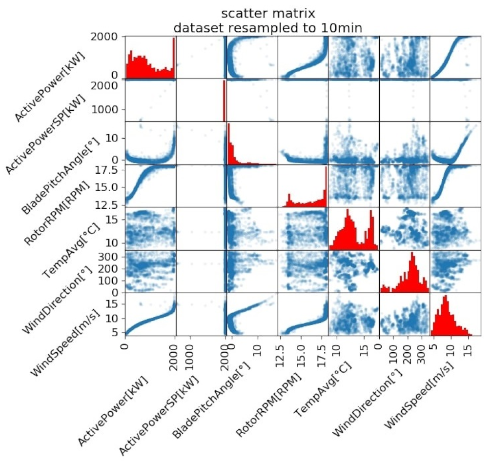
Cross-validated recursive feature elimination (RFECV):

Perform RFECV for each turbine to identify the set of wind turbines that, when used as features for training, yields a model of minimised power prediction error. Briefly mentioned in Section 1, RFE works by iteratively down-selecting features. At each down-selection, a model is trained and the model coefficients corresponding to each feature are stored. The significance of such coefficients used in many regression tasks is that they are indicative of the explanatory power of each feature in regards to the response variable. In the context of this project’s task for example, a highly positive coefficient belonging to a feature would mean that with its increase, an increase in power produced is to be expected. The opposite can be said for a feature possessing a highly negative coefficient: power would be expected to decrease in response to the feature’s increase.

Thus, in RFE, the first model iteration is trained using all features. Using the resultant feature’s coefficients, the least important feature is identified and excluded in the feature set used in the next training iteration. This iterative down-selection is repeated recursively until there are no more features to exclude. Though this approach does not promise a globally minimal solution (as not all possible combinations of features are tested) it provides a computationally efficient means of feature down-selection.

The RFE used in this task was cross-validated; meaning that at each recursive iteration, 10-fold cross-validation was used to determine which feature was least important and discarded in future iterations. To explain explicitly, at each iteration, the dataset is split into 10 folds. The wind turbine model for which RFECV is being performed is then trained on 9 of these folds, and the coefficients corresponding the the different wind turbines (features) are stored. This is repeated for every possible combination of 9 folds within the 10 total folds. The mean of the coefficients across all these combinations of folds (10 coefficients per feature) is taken. Using these coefficient means, the cross-validated least important feature is identified. This feature is discarded in the next recursive iteration and the 10-fold cross validation is repeated. Thus used, cross-validation serves to offer more robust estimates of a feature’s importance, as it is assessed over varied subsets of observations.

The final aspect of the implemented RFECV to be discussed is the regression algorithm used at each recursive elimination to generate the feature coefficients and the choice of data to feed it as input. First, as an ordinary-least squares linear regression model (LR) satisfies the need of RFE for a coefficient-based algorithm as well as offers the simplest and quickest computation, it is selected as the algorithm to use in RFECV. Next, the decision of which feature set to use (wind speed, or wind speed and wind direction) had to be made. As can be observed in Figure 3, wind direction shares a highly nonlinear relationship with power and thus is ill-suited for use in the LR-based RFECV. Accordingly, wind speed was the sole feature chosen for RFECV. Finally, in order to improve the quality of the LR’s fit to the feature’s data, a truncated range of the the power curve of the wind turbine being modelled was used. Specifically, the filtered dataset output from Section 2.3 was only used in the range $<P_{rated}$. This region was selected as it explicitly is more linear than the power curve taken as a whole, and thus presents an input more compatible with the constructed LR-based RFECV.

(2)

Entire WF-informed down-selection cut-off:

After RFECV is performed for every turbine, curves showing number of features vs. cross-validated power prediction error can be generated. Plotting these curves for every turbine demonstrates that though prediction error decreases with the inclusion of more wind turbines as features as earlier hypothesised, there is a common point among turbine models where the benefit seems to diminish. Thus, to strike a balance between model complexity and performance, a feature cut-off of 15 wind turbines was made. To down-select to 15, the absolute value of the set of coefficients for a given model were sorted by value, and the 15 features (wind turbines) possessing the highest coefficients were taken as the most important. Figure 5 with the following visualisation of these curves was used as reference in determination of this cut-off.

Figure 6 serves to represent two characteristically different outcomes of this feature down-selection: The first being a case where the feature cut-off of 15 is much less than the RFECV’s best number of turbines, and the second being where it is closely aligned with the best number of turbines. In the case where best number of turbines was less than the cut-off, the RFECV’s best set was used as it yielded the simplest and highest performing solution.

2.4.4. Regression Model Overview

With the datasets needed for all three model scales now defined, it is possible to use them for training different machine learning algorithms to be tested as the NBM’s regressor.

2.5. Model Selection Rationale

The implementation of machine learning estimators in a programmatic environment like Python makes their application relatively straightforward. However, rather than simply applying many algorithms to the task to see which one prevails, a rationale is considered for using thoughtfully selected algorithms from both a demonstrative and task-specific perspective.

First, an explanation as to why some of the top-most algorithms, as presented in Section 1, were not tested in this project is offered. Certain algorithms, such as SVR and GP, use the kernel trick to learn high-order relationships between explanatory and response variables. This ability to model high-order relationships is essential given the nonlinearity of the power’s relationship with wind speed and wind direction. However, as previously discussed, this trick requires the expansion of the dataset dimensionality that scales with the number of observations in the dataset. Considering the size of datasets considered here, this represents a prohibitive computational-expense. Another common family of regression algorithms not tested here are those that employ regularization, such as in Lasso. Regularized LR models are an extension of linear regression that effectively introduce a tuned amount of bias in the LR’s solution so as to decrease its variance in test set performance. Regularization is thus a primarily useful extension when observations available for training are few, as such a scenario presents the risk of overfitting, or overly biasing, the purely LR solution to understand the dataset. In such a scenario, a model may understand its training data well, but is liable to generalise to new observations poorly. As lack of observations is not an issue in this project, it was decided that the particular benefits of regularized LR methods would not be needed.

Thus, the models that were chose represent a spectrum of abilities either specifically suited for this task or suitable to serve as a baseline regressor that, through its use as a comparative reference, serves to justify the testing of more computationally complex estimators. The baseline regressor tested in this project is least squares LR. The next estimator tested was RF regression (RFR), as it represented an algorithm with the ability to fit to nonlinear relationships without the aforementioned level of computational complexity associated with other methods possessing the ability to make nonlinear fits. Two types of ANN, representing the state-of-the-art family of algorithms considered fit for such a nonlinear task, were also explored. Like LR and RFR, a typical ANN-FF learns to make a prediction for a given observation given only feature values at that single observation. ANN-LSTM however, represents a fundamental recurrent extension from the ANN-FF and the other regressors considered. For it learns to make a prediction for a given observation given the feature values over a preset range of previous observations. As demonstrated by a density of recent relevant studies (some being presented in Section 1), this temporal model extension seemed worthy of testing in this project’s task.

2.5.1. Dataset Transformations

Before being used in the tuning of the described regression models, the explanatory variables (X) in all appropriate datasets were standardized using the following definition:

$$\tilde{X}=\frac{X-{\mu }_X}{{\sigma }_X}$$

(1)

where ${\mu }_X$ and ${\sigma }_X$ are the mean and standard deviation for a given feature of X.

2.5.2. Model Tuning

As performed for the LOF hyperparameter tuning briefly presented in Section 2.3, here each regression model has an array of hyperparameters that can be tuned to better adapt each model to the specific task at hand in an effort to ultimately yield better performance. For all estimators other than the ANN’s, the default hyperparameter settings as defined in their scikit-learn implementations [16] were utilized. This decision was made for a number of reasons. First and foremost, at this initial stage, it was desired to compare models primarily on a high level to see if any were particularly well or ill-suited for the task. Second, upon investigation it was confirmed that the default hyperparameter settings often reflect best-guess starting points for general applications; often times even relating directly to recommendations put forth by the literature which first marked their inception (as seen in Section 2.3 with LOF’s contamination hyperparameter). Third, adequately tuning algorithms can require immense computational complexity, especially so if the training dataset is large, and at 537 k × 553 (observations × features), the dataset at hand in this Section can indeed be considered large [16].

To adequately tune hyperparameters, cross-validation is recommended to avoid making conclusions about their effectiveness based on a narrowed-view of the dataset’s interactions. Then, for example, if for a given estimator it was desired to tune 3 hyperparameters using a moderate 5-point range for each and to further validate the tuning using 10-fold CV, the process would entail $5^3$ × 10 = 1250 iterations of training and testing. Such an exhaustive search for the ideal set of hyperparameters is known as a cross-validated grid search. This grid search performed for 6 different algorithms for 79 turbines at 3 different scales and testing 2 different SCADA tag sets as features sets, further increases the number of iterations needed to tune all models to 1250 × 6 × 79 × 3 × 2 = 3.555 × ${10}^6$ iterations. Last, the final goal of this project was not to determine a globally optimized NBM, but rather to identify an efficient path towards the development of one to be used effectively for the power performance analysis. Accordingly, it was decided to devote less effort to true estimator-optimization in order to allow more time to assess the best estimator’s fitness as a power performance analysis tool.

However, as aforementioned, high-level hyperparameters for ANN-based estimators were subjected to a moderate tuning. This was performed for two reasons. First, unlike the scikit-learn estimators, the Keras [18] front-end/TensorFlow [19] back-end-based ANN models are relatively undefined in regards to recommended defaults to be used for general application. This is less true for some hyperparameters than others, and thus the most important yet undefined hyperparameters in this sense were chosen for a cross-validated grid search to explore whether certain sets best equip the ANN models to perform the task at hand. Second, as presented in Section 1, ANN represents the cutting edge in machine learning regression applications, including those proliferating the wind energy industry. Thus, as it is this project’s desire to also push the cutting edge, it serves benefit to pay an added focus to the ANN estimators so as to ensure they have been adequately equipped to perform on par with the other repressors being considered.

ANN-FF Tuning

Inexhaustive Searches. A CV grid search tests all possible combinations of input ranges for select hyperparameters, and is thus referred to as an exhaustive search. Anything less than this can then be referred to as inexhaustive. Considering the computational expense of a CV grid search as previously described, it was desirable to first perform an inexhaustive tuning of more general hyperparameters affecting model training and testing performance. For ANN-FF, perhaps the highest level hyperparameter determining its architecture is its number of layers. Through empirical tuning, it was decided that 2 hidden layers provided adequate balance of performance and computational complexity across all high level model permutations (i.e., scale and feature sets).

Other hyperparameters inexhaustively tuned were the batch size and epochs used in the ANN-FF’s training. Batch size defines the number of observations to iterate over before the model’s gradient is updated, while epochs defines the number of times the entire set of the dataset’s observations are exposed to the model. Thus, both metrics have a direct effect on the commonly used ANN training evaluation visualisation known as its learning curve. An ANN’s learning curve plots the model’s training and validation error vs the number of epochs over which it was trained. A learning curve is said to be “well fit” if it has both training and validation curves’ error decreasing together over the epochs until either a minima or flatline is reached. However, achieving this well-fit learning curve can require some empirical tuning, and thus was made the goal of these two inexhaustive searches.

By incrementally increasing the batch size from the default of 32 observations, it was found that a batch size of 300 observations offered significant improvement to the ANN-FF’s learning curve. Furthermore, from inspection of the turbines’ learning curves, it was observed that a minimum MAE is reached at approximately the 20th epoch. Thus, an epoch limit of 25 was used with a early callback option that terminated training if the epoch’s validation error did not improve over 2 epochs.

Exhaustive Searches. The parameters for the ANN-FF estimator that were tuned exhaustively using a cross-validated grid search were those defining the ANN’s neurons-per-layer. Here, as opposed its employment in RFECV, a CV of k = 5 folds was used in order to save computational expense. This was considered sufficient given the objective of obtaining a general indication of preferred ANN architecture for the task at hand and the fact that each architecture was tested over the entire wind farm of turbines, thereby providing a layer of hyperparameter semi-validation in and of itself.

The range of neurons-per-layer that were grid searched over were 2, 5, 10, 20, 50 and 100 per layer. Thus, each combination of neurons allocated to each layer provided the ANN a unique architecture. The grid search was performed for each turbine at each model scale and feature set.

From inspection of the grid search, a number of observations were made. First, the most repeatable apparent trend across model scales and feature sets is the decrease of RMSE with an increase in neuron count in layer 2 ($n2$). This is a strong trend from $n2=2$ to $n2=20$, at which point the benefit of additional n2 counts is minimal. Next, it appeared that when using wind speed as the feature set, the model scale performance hierarchy is WFL > WF $>>$ WT. When windspeed and wind direction are used as the feature set, the hierarchy appears to be WFL > WT > WF. These were both surprising results as it was originally hypothesised that WF would outperform the other two model scales for its added information. Finally, it can be observed that across all scales, using a feature set of only wind speed outperforms the use of a feature set using wind speed and wind direction. This is also surprising given the important wake-centric carrying information of the wind direction SCADA signal. It is hypothesised that the poor results were related to the wind direction signal’s relatively high variability.

ANN-LSTM Tuning

The process used to tune the LSTM model was a similar combination of exhaustive and inexhaustive searches over parameter ranges of interest. Inexhaustively, it was found that the same batch size and epochs as determined effective for ANN-FF training were also effective for LSTM model training: 300 observations and 25 epochs.

The following sequence outlines the iterative grid-searching process used to identify suitable hyperparameters for the LSTM-based NBM:

(1)

Layer architecture and preliminary lag search:

The first exhaustive tuning objective was twofold: identify a preferred layer architecture and sequential-input-defining lag time. Here, in the TensorFlow nomenclature, the lag time is equivalent to the number memory cells per block and a block is equivalent to a neuron.

In order to search over both of these hyperparameters, a grid search using a range of lag times 1, 5, 10, 20 and 30 s was implemented for two LSTM-containing ANN architectures:

(a)

2-layer with an LSTM hidden layer

(b)

3-layer with an LSTM hidden layer connected to a fully connected, dense feedforward-style hidden layer.

Though architecture (b) is less common, it was thought worthy to explore given the anecdotal performance improvement of the utilization of 2-hidden layers in the ANN-FF tuning. Further, as demonstrated in [20], such an architecture is particularly capable of learning sequences that are conditional to constraints, such as a power signal conditional to wind turbine operational constraints.

From inspection of the validation results between architectures (a) and (b) trained using different lag times, two main observations could be made: First, it appears that the LSTM + Dense network significantly outperforms the single LSTM layer network, scoring a median min RMSE of approximately 150 kW across all turbines, while the single LSTM layer architecture scoring a median min of 350 kW. Second, it was observed that for both architectures, performance improves with added lag time; between 1 to 5 s for LSTM and apparently up to the range max of 30 s for the LSTM + Dense architecture.

Based on these results, an extended lag study was performed using the LSTM + Dense architecture for all scales to further investigate a best-suited value for this hyperparameter.

(2)

Extended lag study using best layer architecture:

Here, a range of 1, 5, 10, 20, 30, 45 and 60 s were tested for each model scale, all at the preferred LSTM + Dense architecture.

From inspection of this study’s results, a number of observations can be made. First, it was seen that the WT scale model is the primary beneficiary of the extended lag time tested in this search; with performance continuing to significantly improve up until lag = 45 s. Next, it was seen that the WFL scale improves from 1 to 20 s, with no significant change beyond this point (except perhaps an increase in variance between 20 to 60 s). These trends are also exhibited generally by the WF scale. Finally, it was seen that all models achieve similar median min RMSE at their best lag, with the minimum overall median score belonging to the WFL scale using lag = 20 s.

Thus, a lag of 20 s was selected as a balance of performance and computational complexity.

(3)

Neuron grid search for all scales using best lag time:

To check the ANN-FF-tuning-based assumption of 20 neurons being best, a grid search was again performed to search over combinations of neurons for both the LSTM and dense, feedforward layers. As in the ANN-FF grid search, here a 5-fold cross-validation was used. Here, note that $n1$ corresponds to the number of neurons in the LSTM layer, while $n2$ corresponds to those in the dense feedforward layer.

From inspection of this grid search’s results, a number of observations could be made. First, the WFL was shown to outperform the WF and WT models; a surprising result given the findings of the ANN-FF neuron grid search. Second, for the WT model, a neuron set of $n1$ = 50, $n2$ = 50 proved best while $n1$ = 20, $n2$ = 20 proved best for WFL and WF models. The fact that these results were monotonically decreasing with lower neuron counts unto the minimum tested in this range motivated a follow-up grid search representing neuron counts of even lower values.

(4)

Lower range extended neuron grid search at best model scale (WFL):

Here, an extended neuron range of $n1,n2=2,5,10$ neurons was tested for only the best performing model scale of WFL.

From inspection of this extended search, it was seen that a combination of $n1=5$, $n2=20$ yielded the best performing model. Thus it is chosen as the neurons-per-layer hyperparameter with which to train the final LSTM-based regression models.

Summary of Selected ANN-FF & ANN-LSTM Hyperparameters

Table 3. Summary of the ANN-FF and ANN-LSTM model parameters selected through tuning.

		Layer 1			Layer 2
Model	Lag [s]	Type	n	Activ. Func.	Type	n	Activ. Func.	Optimizer	Loss	Batch Size	Epochs
ANN-FF	NA	dense	20	relu	dense	20	relu	adam	MSE	300	25
ANN-LSTM	20	LSTM	5	-	dense	20	relu	adam	MSE	300	25

offers a summary of the selected ANN-FF and ANN-LSTM model parameters:

2.5.3. Comparison of Tuned Regression Model Performance

With hyperparameters established for all the regressors, it is now possible to compare their performance in order to choose the one best suited for the power performance analysis objective of this project. The performance metrics for this comparison were generated using a 10-fold cross validation for each model. Such a metric thus serves to describe each model’s generalised performance, i.e., that which it would exhibit when given hitherto unseen observations. This is pertinent in this project as the test set (detailed in Section 2.2) to be subjected to this project’s power performance analysis will not be exposed to these regressors until the performance analysis itself. For this comparison’s 10-fold CV, each regressor was trained at each model scale and using each feature set. As separate scripts were written for separate models, seeding the randomness of the CV function ensured models were evaluated over the same folds.

Table 4. Model comparisons in which wind speed, and wind speed and wind direction, were used in the feature set. Values represent medians across all turbines. Note that LSTM was not tested using the wind speed and wind direction feature set as at time of its training, results strongly suggested wind speed only as the superior feature.

		MAE [kW]			RMSE [kW]			Training Time [min]
Model	Feature	WT	WFL	WF	WT	WFL	WF	WT	WFL	WF
LR	WS	173.8	155.7	165	226.7	209.5	218	0.0002	0.01	0.08
RFR	WS	115.9	88.9	85.3	166	129	125.6	0.15	1.91	12
ANN-FF	WS	117.5	94	86.8	166	135.3	124.3	2.75	2.7	2.7
ANN-LSTM	WS	86.8	74.4	78.3	126.2	110.8	115.5	6.8	6.6	6.3
LR	WS + WD	175.6	152.5	153.9	227.8	203	207.6	0.02	0.09	0.4
RFR	WS + WD	140.7	92	95.5	198.8	131.7	132.8	0.3	4.3	14.7
ANN-FF	WS + WD	123.8	97.8	113.7	172.3	132.8	155.3	2.9	2.9	2.8

offers a summary of the model comparisons.

As can be seen, RFR and both ANN variants far outperform the base LR reference regressor across all scales, feature sets, and error metrics (RMSE and MAE). Next, it can be seen that for all models, only using wind speed in the feature set provides better performance than when wind speed and wind direction are used in the feature set. Finally, for all regressor types other than ANN-FF, the WFL scale yields the highest performing models.

At the WFL scale using wind speed in the feature set, ANN-LSTM achieves the lowest median MAE (across all turbine models) of 74.7 kW with the next closest model at this scale (RFR) achieving a median MAE of 88.9 kW.

Thus, the ANN-LSTM WFL scale model using only wind speed in the feature set is selected as the best model to use in the NBM with which to perform the power performance analysis.

2.6. Trained Model Inspection

2.6.1. Definition of Residual

The definition of residuals used in this study’s power performance analysis aligns with the following definition:

$$residual=y_i-{\tilde{y}}_i$$

(2)

where $y_i$ is the actual value of the response variable at observation i and ${\tilde{y}}_i$ is the model’s prediction at observation i. This precise definition aligns the residual signal intuitively with the direction of abnormal performance—for a negative residual will correspond to a suspect case of under-performance while a positive residual will correspond to a suspect case of over-performance.

2.6.2. Residual Inspection

Before embarking on using the now trained NBM’s in a power performance analysis, it is important to inspect the trained models in an effort to inform the analysis. Specifically, understanding the model’s levels of uncertainty and bias must factor in to any conclusions made through the analysis. Further, when inspected in wind farm and power curve space, they can offer insight as to how the turbines might behave in the test set and also where the models struggled to capture the behaviour of the wind turbines in the training set. This can then, for instance, serve to educate further training sessions if refinement of the final power performance analysis on the test set is desired.

The residuals inspected in this section are of each trained wind turbine’s predictions given the training set data used in its training. The distributions of these residuals for all turbines individually were plotted and inspected. Additionally, in order to inspect the range of uncertainties and biases at a higher level, the training residual means and standard deviations are plotted in wind farm-space:

2.6.3. Bias Inspection

From observation of Figure 7a, it can be seen that the turbines exhibiting the highest negative residual bias are located deep within the wind farm considering the predominant wind direction in the dataset (230${}^{\circ }$ with reference to Figure 3) while those exhibiting the highest positive residual bias are along the outer perimeter without respect to the predominant wind direction. In this project’s context, a negative bias indicates the model has an innate bias to diagnose a wind turbine as underperforming while a positive bias denotes a bias to diagnose as overperforming. Considering that the models used here were at the WFL scale, in which other turbine’s wind speed SCADA data was used as model features, it is possible that these biases correspond to the models’ struggle to model the wake effect at play within the farm. For instance, consider WT12, which exhibits perhaps the highest positive bias. From discussion in Section 2.4.3, it is known that its model uses wind speed signals from neighbouring turbines to predict its own power. Considering that the particular neighbours for WT12 are those that are both along the perimeter of the farm and at the most upstream locations relative to the predominant wind directions, it is likely that the models overly trusted these higher wind speed signals in predicting the power of WT12; that is to say, the model underestimated the wake effect occurring between WT12 and its upstream neighbours. Applying a similar rationale, it conversely appears that the WFL model for WT62 underestimates the wake effect between it and its neighbours. This is perhaps for two reasons, both relating to the bimodal nature of the dataset’s wind direction distribution. For at the predominant peak the wake experienced by WT62 should be among the highest in the wind farm as its at an approximate downstream depth of six turbines. However, at the distribution’s secondary peak (centred approximately at 320${}^{\circ }$), the wake effect experienced by WT62 should be among the lowest in the wind farm at a downstream depth of 1 turbine. Thus, a model trained on such a bimodal data would indeed exhibit a negative bias when tested on the same dataset.

2.6.4. Variance Inspection

In Figure 7b, the standard deviation of the wind turbines’ residuals is visualised in wind farm space. Here, a trend can be observed in which the wind turbines located mainly upstream relative to the dataset’s predominant wind direction show lower standard deviation than those downstream. This is likely directly related to the difference in turbulent intensity in the wind field felt by upstream vs. downstream turbines as discussed in Section 2.3.2. In the context of residuals, it is inferred that a model trying to describe the nature of something possessing a higher level of variance is in turn likely to yield a higher level of residual variance. In this figure, it can also be observed that WT51 seemingly opposes this trend; possessing a lower standard deviation than its neighbours and wake-related position would suggest. It is likely that the bimodal nature of the wind direction is again at play, considering that at the distribution’s secondary peak (320${}^{\circ }$), WT51 should experience minimal wake effect and associated turbulent intensity and consequently should exhibit minimal variation in its model’s residuals.

3. Results and Discussion

3.1. Test Set Power Performance Analysis

With the models trained and inspected, and analysis guiding control limits set, it is now possible to employ the models in a power performance analysis on the hitherto unseen test set discussed in Section 1. As a final step, the test set is filtered using filters similar in definition to the operational filters applied to the training set but differing here in their application’s intent.

3.1.1. Test Set Filtration

Whereas when applied to the training set the operational filters were used in an effort to define normal turbine behaviour, here, the application to the test set serves to filter out observations considered not-of-interest to the objectives of the power performance analysis. Specifically, such observations can fall into two categories: those representing false positives and those representing behaviour outside of the range of expected normal behaviour.

(1)

False positive here denotes observations that, given the model’s trained definition of normality, would yield high indication of abnormality through high residuals, but yet the nature of which is not of interest in the analysis. Here, instances of downregulation would yield false positives and are thus filtered.

$$\mathrm{ActivePowerSP}<2000\mathrm{kW}$$

(3)

(2)

In filtering out observations representing behaviour outside of the nominal bounds of normality, a similar such filter as applied to the training set is considered. However, here conditions are modified slightly in order to preserve observations that, though outside of operational bounds, may indicative of instances of of under or over performance.

$$\begin{array}{c}(\mathrm{WindSpeed}<4\mathrm{m}/\mathrm{s})\\ \mathrm{OR}\\ \left(\right(\mathrm{WindSpeed}<4\mathrm{m}/\mathrm{s}\left)\mathrm{AND}\right(\mathrm{ActivePower}<66.6\mathrm{kW}\left)\right)\\ \mathrm{OR}\\ (\mathrm{WindSpeed}>25\mathrm{m}/\mathrm{s})\end{array}$$

With these filters established, they were applied to the test set corresponding to the WFL scale model for each turbine which was then fed directly as input into each turbine with which to generate test set predictions.

3.1.2. Mitigating Test Set Residual Uncertainty

With the NBM predictions made for the test set, it is now possible to analyse the time series of their residuals. In order to increase the confidence in the signal, and thereby increase confidence in conclusions regarding performance abnormalities, a rolling mean of the signal was applied as in [2]:

$$e_{roll}\left(i\right)=\frac{1}{2\eta +1}\sum _{j=0}^{2\eta }e(i+\eta -j)$$

(4)

where $e_{roll}\left(i\right)$ is the rolling mean error at time i, e is the raw error signal and $\eta$ is the window size defining the number of observations over which to calculate the mean for observation i. A window size of $\eta$ = 60 s was used as it aligns with conventionally used time scales and was empirically found to work well for this project’s analysis task. With the application of the rolling mean using this window size, the resultant residual signal provides a more robust measure of performance without washing out the signal at high frequencies. From inspection of the rolling means’ effect on residual distribution, it could be seen that increasing the window size decreases signal uncertainty incrementally.

3.1.3. NBM Results

Finally, it is possible to analyse the signal of the NBM’s residuals in an effort to analyse the power performance of the turbines over the course of time represented by the test set. This section will first present a joint time series of all the wind turbines NBM’s residuals with the wind farm-wide control limits superimposed for reference. Here, individual select cases of abnormal performance are annotated then individually investigated in the following sections.

The joint residual time series for all turbines over the test set is presented in Figure 8 with select cases annotated.

Proof of Concept—WT94

In this section, an abnormal event associated with gross under-performance of a wind turbine, in which the turbine appears to be out of operation, is investigated. As it offers a definitive case of under-performance, it is considered an easy proof of concept bench test for the model as it is intended to function.

Figure 9 offers semi-continuous time series of the actual and predicted power output of WT94 and their associated residuals. Note the four discrete plots correspond to the four continuous time spans given by the raw dataset.

As can be seen in Figure 9, the wind turbine initially appears to be performing normally as indicated by the rolling means maintaining itself generally about zero and within the control limits. However, at approximately 10-21 01:00:00, the residual drops sharply to a minimum of $-2000$ kW. By observing the plot of actual and predicted powers, it becomes clear that the turbine has simply entered a state of non-operation while its model continues to predict power as if it were still in operation. Considering that non-operating state corresponds to a power output of 0 kW, the residual of $-2000$ kW suggests that the turbine would have been likely producing power at its rated state if it were indeed operational.

Under-Performance Case—WT25

In addition to the time series of predicted vs. actual power and the associated residuals, the select case of abnormal power performance presented in Figure 8 was investigated from two other perspectives. First, as the NBM’s residuals represent the degree of a turbine’s abnormality relative to its previously established normal behaviour, the abnormal event is investigated in power curve space in which both the normal and abnormal traces of power performance for the given turbine can be compared. Second, to investigate the event’s degree of abnormality relative to other wind turbines in the farm, a contour snapshot of the wind farm power output delivered at the observation of max abnormality is generated. Here, arrows indicating the wind direction signal recorded at each wind turbine also offer insights informing root cause hypotheses.

In Figure 10a, the investigated under-performance case for WT25 can be seen to occur at approximately 11-10 11:00:00, at which point the rolling average residual signal surpasses the turbine’s LCL of 3$\sigma$, reaching a minima of $-909$ kW in the 60 s rolling mean residual signal. In the power time series itself, it appears the actual and predicted series drops sharply from rated power to approximately 500 kW then returns sharply again to rated.

The under-performance event is investigated further in the turbine’s power curve space in Figure 10b. Here, the time scale of the event is explored at a finer resolution, where it can be seen that the abnormal event spanned approximately 1 min from 11:22 to 11:23 ($t_{abnormal}$). The time-consecutive power curve observations within $t_{abnormal}$ are indicated as orange scatter points, and they offer a trace of how the power changed within $t_{abnormal}$ relative to WT25’s power curve observations for the rest of the test set ($t_{all}$). This trace shows that the within 1 min, the power rapidly decreased from slightly above rated to approximately 300 kW, at which point the minimum raw residual of $-1633$ kW was produced. By visual inspection, the gap between this minimum and WT25’s binned average power curve at this wind speed is approximately $2000-300$ kW = 1700 kW, which aligns closely with the residual and its standard uncertainty (coverage factor k = 1) of ${\sigma }_{train}$ = 114 kW (as seen in Figure 10a’s legend).

Finally, the event is investigated in wind farm-space in Figure 10c. Here, it can indeed be seen that WT25 is under-performing abnormally relative to the other turbines at the timestamp of its minimum residual, with most other turbines producing over 1800 kW. The wind farm-wide wind field as portrayed by the wind direction indicating arrows is unique in that there appears two main directions flowing through the farm: One at approximately 310${}^{\circ }$ and the other at approximately 280${}^{\circ }$. It should be noted here that, as visible in Figure 10c, a number of turbines’ wind direction signals were repeatably found to be offset relative to the majority, and are thus are assumed to be out of calibration for the duration of the dataset used. Without venturing too deeply into root cause analysis, the scope of which is beyond this project, it is postulated that this duality in wind direction perhaps confused the turbine’s yaw controls so as to momentarily yaw to a sub-optimal power producing position.

Over-Performance Case—WT62

In Figure 11a, the investigated over-performance case for WT62 can be seen to occur at approximately 10-21 06:00:00, at which point the rolling average residual signal surpasses the turbine’s UCL of 3$\sigma$, reaching a maxima of 670 kW in the 60 s rolling mean residual signal. In the power time series itself, it appears the actual and predicted series rapidly increase from 300 kW to rated then rapidly decrease back to an output of approximately 500 kW.

The over-performance event is investigated further in the turbine’s power curve space in Figure 11b. Here, the time scale of the event is explored at a finer resolution, where it can be seen that the abnormal event spanned approximately 6minutes from 06:24 to 06:30 ($t_{abnormal}$). The time-consecutive power curve observations within $t_{abnormal}$ are indicated as orange scatter points, and they offer a trace of how the power changed within $t_{abnormal}$ relative to WT62’s power curve observations for the rest of the test set ($t_{all}$). This trace shows that the within 6 min, the power increased from 1250 kW to approximately 2000 kW, at which point the maximum raw residual of 979 kW was produced. By visual inspection, the gap between this maximum and WT62’s binned average power curve at this wind speed is approximately $2000-1000$ kW = 1000 kW, which closely aligns with the residual value and its standard uncertainty (coverage factor k = 1) of ${\sigma }_{train}$ = 118 kW (as seen in Figure 11a’s legend).

Finally, the event is investigated in wind farm-space in Figure 11c. Here, it can indeed be seen that WT62 is over-performing abnormally relative to the majority of turbines at the timestamp of its maximum residual, though its immediate neighbours also seem affected. Again, there appears to be a “streak” of over-performance, this time exhibited by the two turbines due West of the investigated turbine. Due to these three turbines’ proximity to the out-of-operation WT32, it is possible that (though this snapshot’s wind direction vectors are not in precise support) the wind speed reduction caused by the wake produced by turbines upstream to these three over-performers has been able to recover over this open-fetch to provide these three with an abnormally high wind speed given their location in the wind farm and the wind direction vectors at this timestamp.

4. Conclusions

This study has demonstrated an approach to wind turbine power performance analysis using regression-based normal behaviour modelling.

In this approach, it was demonstrated that the WFL model scale, in which only turbines correlated with the turbine to be modelled were sourced for SCADA tags, ultimately provided results superior to single turbine-sourced scale (WT) and even the entire wind farm-sourced scale (WF). Further, it was found that a uniquely structured machine learning ANN regressor possessing both an LSTM and feedforward layer outperformed all other algorithms in the power prediction objective, including models using ANN-FF and ANN-LSTM explicitly. Finally, through the successful identification of instances of abnormal performance as presented in the test set’s power performance analysis, this study’s 2-tiered process of defining normality for each turbine is empirically validated.

Despite its demonstrated effectiveness, there are aspects of the proposed NBM that can likely be improved. First, it is suggested that the abnormality–filtration sequence (used to define normal behaviour for each turbine) be tied directly to the residual output of the regression model. Such a combination of machine learning techniques is referred to as a pipeline, and it is commonly used to tune the hyperparameters of upstream algorithms given the output of a downstream algorithm. In the context of this project, a proposed pipeline might be to tune the LOF’s n-neighbours and contamination parameters so as to minimize the training residual-based regressor model uncertainties. Another suggestion for potential improvement to the NBM is to narrow the model’s range of focus with regards to the power curve; namely excluding power above the threshold represented by rated power. The inclusion of this range in this project conceptually enabled identification of both under- and over-performance represented by this range, but in practice the NBM struggled to model power production here, especially at higher wind speeds (as evinced in Section 2.6). This led to a contamination of the residual signals’ meaningfulness; where the model’s inability to accurately maintain rated power frequently manifested as false under-performance events. Further, where this project identified singular model thresholds and hyperparameters deemed suitable to the wind farm as a whole (for simplicity’s sake), it is entirely possible that a purely data-driven tuning of models on an individual wind turbine basis could provide even stronger NBM’s than those chosen as best in this study. Finally, to provide a level of oversight and reliability, monitoring the model’s wind turbine performance metric using a complexity indicator such as entropy could be implemented as in [21].

References

- Lapira, E.; Brisset, D.; Davari Ardakani, H.; Siegel, D.; Lee, J. Wind turbine performance assessment using multi-regime modeling approach. Renew. Energy 2012, 45, 86–95. [Google Scholar] [CrossRef]
- Colone, L.; Reder, M.; Dimitrov, N.; Straub, D. Assessing the Utility of Early Warning Systems for Detecting Failures in Major Wind Turbine Components. J. Phys. Conf. Ser. 2018, 1037, 032005. [Google Scholar] [CrossRef]
- Gonzalez, E.; Stephen, B.; Infield, D.; Melero, J.J. Using high-frequency SCADA data for wind turbine performance monitoring: A sensitivity study. Renew. Energy 2019, 131, 841–853. [Google Scholar] [CrossRef] [Green Version]
- Colone, L.; Reder, M.; Tautz-Weinert, J.; Melero, J.J.; Natarajan, A.; Watson, S.J. Optimisation of Data Acquisition in Wind Turbines with Data-Driven Conversion Functions for Sensor Measurements. Energy Procedia 2017, 137, 571–578. [Google Scholar] [CrossRef]
- Herp, J.; Pedersen, N.L.; Nadimi, E.S. Wind turbine performance analysis based on multivariate higher order moments and Bayesian classifiers. Control. Eng. Pract. 2016, 49, 204–211. [Google Scholar] [CrossRef]
- Göçmen, T.; Giebel, G. Data-driven Wake Modelling for Reduced Uncertainties in short-term Possible Power Estimation. J. Phys. Conf. Ser. 2018, 1037, 072002. [Google Scholar] [CrossRef]
- Bach-Andersen, M.; Rømer-Odgaard, B.; Winther, O. Flexible non-linear predictive models for large-scale wind turbine diagnostics. Wind Energy 2017, 20, 753–764. [Google Scholar] [CrossRef]
- Papatheou, E.; Dervilis, N.; Maguire, A.E.; Antoniadou, I.; Worden, K. A Performance Monitoring Approach for the Novel Lillgrund Offshore Wind Farm. IEEE Trans. Ind. Electron. 2015, 62, 6636–6644. [Google Scholar] [CrossRef] [Green Version]
- Schlechtingen, M.; Ferreira Santos, I. Comparative analysis of neural network and regression based condition monitoring approaches for wind turbine fault detection. Mech. Syst. Signal Process. 2011, 25, 1849–1875. [Google Scholar] [CrossRef] [Green Version]
- Cardinaux, F.; Brownsell, S.; Hawley, M.; Bradley, D. Modelling of Behavioural Patterns for Abnormality Detection in the Context of Lifestyle Reassurance; Lecture Notes in Computer Science (including subseries Lecture Notes in Artificial Intelligence and Lecture Notes in Bioinformatics); Springer: Heidelberg/Berlin, Germany, 2008. [Google Scholar] [CrossRef] [Green Version]
- Japar, F.; Mathew, S.; Narayanaswamy, B.; Lim, C.M.; Hazra, J. Estimating the wake losses in large wind farms: A machine learning approach. In Proceedings of the 2014 IEEE PES Innovative Smart Grid Technologies Conference, ISGT, Washington, DC, USA, 19–22 February 2014. [Google Scholar] [CrossRef]
- Gonzalez, E.; Stephen, B.; Infield, D.; Melero, J.J. On the use of high-frequency SCADA data for improved wind turbine performance monitoring. J. Phys. Conf. Ser. 2017, 926, 012009. [Google Scholar] [CrossRef]
- Schlechtingen, M.; Santos, I.F.; Achiche, S. Wind turbine condition monitoring based on SCADA data using normal behavior models. Part 1: System description. Appl. Soft Comput. J. 2013, 13, 259–270. [Google Scholar] [CrossRef]
- Kusiak, A.; Zheng, H.; Song, Z. On-line monitoring of power curves. Renew. Energy 2009, 34, 1487–1493. [Google Scholar] [CrossRef]
- Jia, X.; Jin, C.; Buzza, M.; Wang, W.; Lee, J. Wind turbine performance degradation assessment based on a novel similarity metric for machine performance curves. Renew. Energy 2016, 99, 1191–1201. [Google Scholar] [CrossRef]
- Pedregosa, F.; Varoquaux, G.; Gramfort, A.; Michel, V.; Thirion, B.; Grisel, O.; Blondel, M.; Prettenhofer, P.; Weiss, R.; Dubourg, V.; et al. Scikit-learn: Machine learning in Python. J. Mach. Learn. Res. 2011, 12, 2825–2830. [Google Scholar]
- Breuniq, M.M.; Kriegel, H.P.; Ng, R.T.; Sander, J. LOF: Identifying density-based local outliers. In Proceedings of the 2000 ACM SIGMOD International Conference on Management of Data, Dallas, TX, USA, 16–18 May 2000. [Google Scholar] [CrossRef]
- Chollet, F. Keras.Io. In Keras: The Python Deep Learning Library; GitHub: San Francisco, CA, USA, 2015. [Google Scholar]
- Abadi, M.; Barham, P.; Chen, J.; Chen, Z.; Davis, A.; Dean, J.; Devin, M.; Ghemawat, S.; Irving, G.; Isard, M.; et al. TensorFlow: A system for large-scale machine learning. In Proceedings of the 12th USENIX Symposium on Operating Systems Design and Implementation, OSDI 2016, Savannah, GA, USA, 2–4 November 2016. [Google Scholar]
- Makris, D.; Kaliakatsos-Papakostas, M.; Karydis, I.; Kermanidis, K.L. Combining LSTM and feed forward neural networks for conditional rhythm composition. Commun. Comput. Inf. Sci. 2017, 744, 570–582. [Google Scholar] [CrossRef]
- Huo, Z.; Martínez-García, M.; Zhang, Y.; Yan, R.; Shu, L. Entropy Measures in Machine Fault Diagnosis: Insights and Applications. IEEE Trans. Instrum. Meas. 2020, 69, 2607–2620. [Google Scholar] [CrossRef]