Abstract
This article discusses the optimization of railway transition curves, through the application of polynomials of 9th and 11th degrees. In this work, the authors use a 2-axle rail vehicle model combined with mathematically understood optimization methods. This model is used to simulate rail vehicle movement negotiating both a transition curve and circular arc. Passenger comfort is applied as the criterion to assess which transition is actually is the best one. The 4-axle vehicle was also used to verify the results obtained using the 2-axle vehicle. Our results show that the traditionally used in a railway engineering transition—3rd degree parabola—which is not always the optimum curve. This fact is especially valid for the longest curves, with lengths greater than 150 m. For such cases, the transition curves similar to standard curves of 9th and 11th degrees is the optimum ones. This result is confirmed by the use of the 4-axle vehicle.
1. Introduction
Today, transport negatively influences both the environment and human health. It is also a big energy consumer. Due to this fact, engineers tend to project sustainable transport systems with a smaller negative impact on health and ecosystems. In railway engineering, the infrastructure, train speed, and train dynamics influence train energy consumption. If we take into account infrastructure 3D shape, it has a big impact on dynamics, and dynamics of train strongly influences journey comfort.
The main aim of this study is the optimization and the shape assessment of the railway transition curves. The authors of the current article have used two advanced rail vehicle models, using the full dynamics of the vehicles, to find new better shapes of railway transitions, not used in the engineering practice. The dynamics of a full vehicle-track system, which means the complete description of the vehicle interactions with the railway track, is still not very popular. The idea to represent the whole rail vehicle with a mathematical point today is not sufficient. The simplicity of the rail model makes that the full examination of vehicle dynamics is impossible. The advanced vehicle model gives the chance of better assignment of dynamical properties of railway transitions to freight or passenger vehicles. The mentioned approach will include criteria for the assessment of transitions other than the comfort of the passengers. For the cargo trains, the main criterion can be the wear in wheel-rail contact.
The authors of [1,2] have shown that using tools, which are characteristic for the railway vehicle dynamics in the shape assessment of the railway transition curves, can give many advantages. It may provide new information not available applying the classical approach treating all elements of the system as the mathematical point. The results of the simulations obtained, using such a method, are not always the same as the results obtained using the classical approach. The mentioned works have concluded that the simulation methods (used by the advanced vehicle models) can be at least a complement to the traditional method. This relates particularly to new high-speed railway lines, where types of rail vehicles operating are specified. Simulation (numerical) studies can find a certain justification, since there are today many software packages of AGEM type (automatic generation of the equations of motion) for railway vehicles. The programs of the lead author for the fast construction of mathematical models of these vehicles are also included.
Up-to-date, in road engineering, the clothoid [3] is the curve most frequently used by engineers. The characteristic feature of this curve is the fact that in this curve, a linear change of its curvature k is a function of the curve length l exists. So, a relatively gradual increase in the lateral acceleration of the rail vehicle can be expected. The Equations for x and y coordinates in a function of l are as follows:
In Equations (1) and (2), C is the constant being the product of circular arc radius and the total curve length.
In railway engineering, the engineers use the simplification of the clothoid. This simplification is the 3rd degree (cubic) parabola. In such an approach, simplification x = l is applied, so the Equation (2) has the following form:
The curve (3) has the linear curvature, because the simplification k = d2y/dx2 is also applied. If we use the exact formulae for the curvature [3], mentioned linearity of the curvature is not to be a fact at the end of the curve.
2. Literature Survey
Today, we may observe a large number of works, which deal with searching for new shapes of transition curves. It has a strong connection, especially in the context of new high-speed train lines construction. In the light of high-speed trains is also visible [4,5,6,7,8]. If we study literature related to railway transition curves formation, we state that a clear division of work is visible. Four groups of the works can be defined, and some works can be presented here as the typical works from each group [9,10,11,12].
The first group is represented by Tari and Baykal. The authors of [9] defined the so-called lateral change of acceleration (LCA) of railway vehicles while negotiating the transition curve as the key criterion for evaluating journey comfort in the railway transition curve. The continuity in time of function of lateral change of acceleration must be absolutely provided. They searched only for the transition curves, which satisfied this condition. Moreover, Hasslinger [13] imposed this condition on LCA.
The second group is represented mainly by the authors of [10]. It is arising from the fact that the advanced model of a railway vehicle (simulation software) was used to assess the dynamical properties of the most popular transition curves used in railway engineering. The authors of [10] took some of the most important dynamical characteristics like lateral and vertical acceleration of vehicle body, wheel/rail lateral and vertical forces, and derailment coefficient to compare the shapes of the transition curves. The same idea can also be found in the work by authors of [14,15,16,17,18,19,20,21,22,23,24,25,26].
The third group is the group, where the properties of transition curves are studied, treated the curve as the mathematical object with all its mathematical properties. In such a group of works, authors mostly try to find the curves better than the 3rd degree parabola (the clothoid) [11,27,28,29,30,31,32].
From the perspective of the impact of the infrastructure shape on passenger comfort is the work [12] by Kufver. Due to this fact, he used the famous European standard elaborated by CEN [33]. In mentioned standard, the percentage PCT of both seating and standing passengers with discomfort feelings was described by the proper Equation. The values of PCT had a form of the 2nd degree parabola in the function of the curve length, and it was mathematically possible to find such a value of the length of the curve, for which the percentage had a minimum value.
Analyzing the literature, one can state that the works where the full dynamics of the vehicle-track system and optimization methods are used jointly are not popular. The classical approach to track-vehicle interactions is still applied [34]. A relatively simple vehicle model (or sometimes just simply a point) and the maximum value of unbalanced lateral acceleration and its change, which should not be exceeded as the demand is still rare. The approach in which during the transition curve shape optimization the advanced rail vehicle model of the vehicle-track system and mathematically understood optimization methods are used is still a certain novelty.
3. Method
As the transition curve, the polynomial of 9th and 11th degrees was applied. High degrees of polynomials were chosen, due to the flexibility of shape modeling. Odd degrees were used, taking into account the fact that such curves have only one so-called standard curve. General Equations for curve, curve curvature, cant, and inclination of superelevation ramp used is:
where:
y—transition curve offset [m],
n—degree of the polynomial,
R—curve radius [m],
l0—total curve length [m],
l—curve current length [m],
k—curvature [1/m],
h—superelevation ramp (cant) [m],
i—inclination of the superelevation ramp [-].
For each characteristic, fundamental geometrical demands in the extreme points of the curve were used [34]. For example, for curvature function mentioned demand is:
- -
- The value of curvature in the beginning point of the curve—0,
- -
- The value of curvature in the last point of the curve—1/R.
In this work, one criterion for transition curve assessment is used. This a normalized integral of the lateral acceleration of the vehicle body along the route. Using the Equation, we have:
where:
QF1—quality function,
Lc—total length of the route [m],
—lateral acceleration of vehicle body [m/s2],
L—current curve length [m].
This criterion is a fundamental criterion in railway dynamics, since vehicle dynamics improvement is guaranteed after the optimization.
The length of the curve was calculated, using the traditional method, known in engineering practice [34]. In this work, two standard curves of 9th and 11th degrees were used as the initial ones. These curves are:
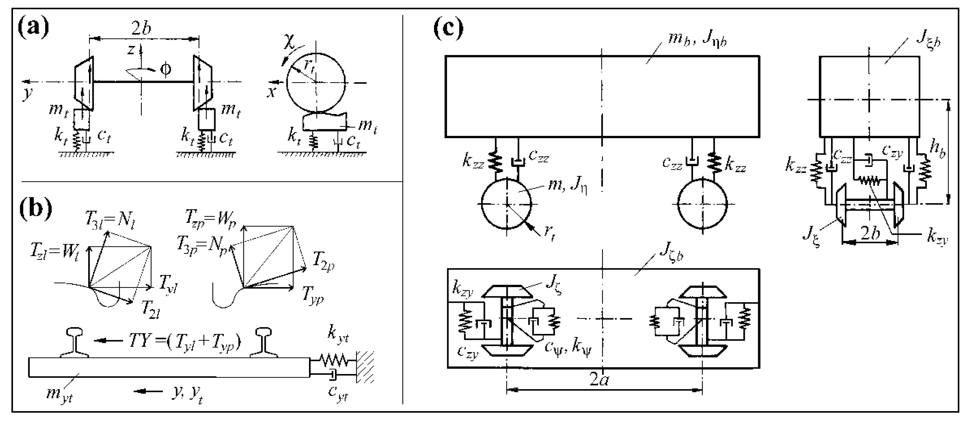
In this work, two models of rail vehicles were applied. The first model has a 2-axle structure. In many earlier works [26], it was called a “2-axle (freight) wagon”. Like every wagon of this type, it has a body connected with two wheelsets with spring-damping elements. The structure of the model and its parameters correspond to a typical real wagon. This model is of key importance here, because in this work, it was used to investigate the dynamical properties and optimize the shape of the transition curves. The nominal model of this vehicle is shown in Figure 1c. The vehicle model is supplemented with the model of the track, as presented in Figure 1a,b. The entire track-vehicle system is discussed in detail [26]. The model parameters of this system are also presented by the authors of [26].
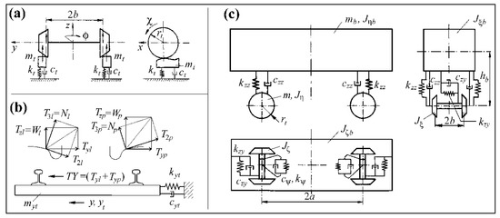
Figure 1.
2-axle vehicle model: (a) Track vertically, (b) track laterally, (c) vehicle.
The second model is MK-111 [26]. This car is a British passenger car. It was used in this work to verify the results of optimization of the shape of transition curves made with the previous model. The nominal model of this vehicle is shown in Figure 2. The parameters of a bogie for this wagon were adopted by the authors of [26]. The remaining model parameters were adopted on the basis of the obtained data at British Rail Research, Derby. The model itself consists of seven rigid elements. The track model included in the vehicle was identical to that for a 2-axle car.
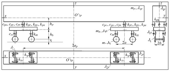
Figure 2.
4-axle vehicle model.
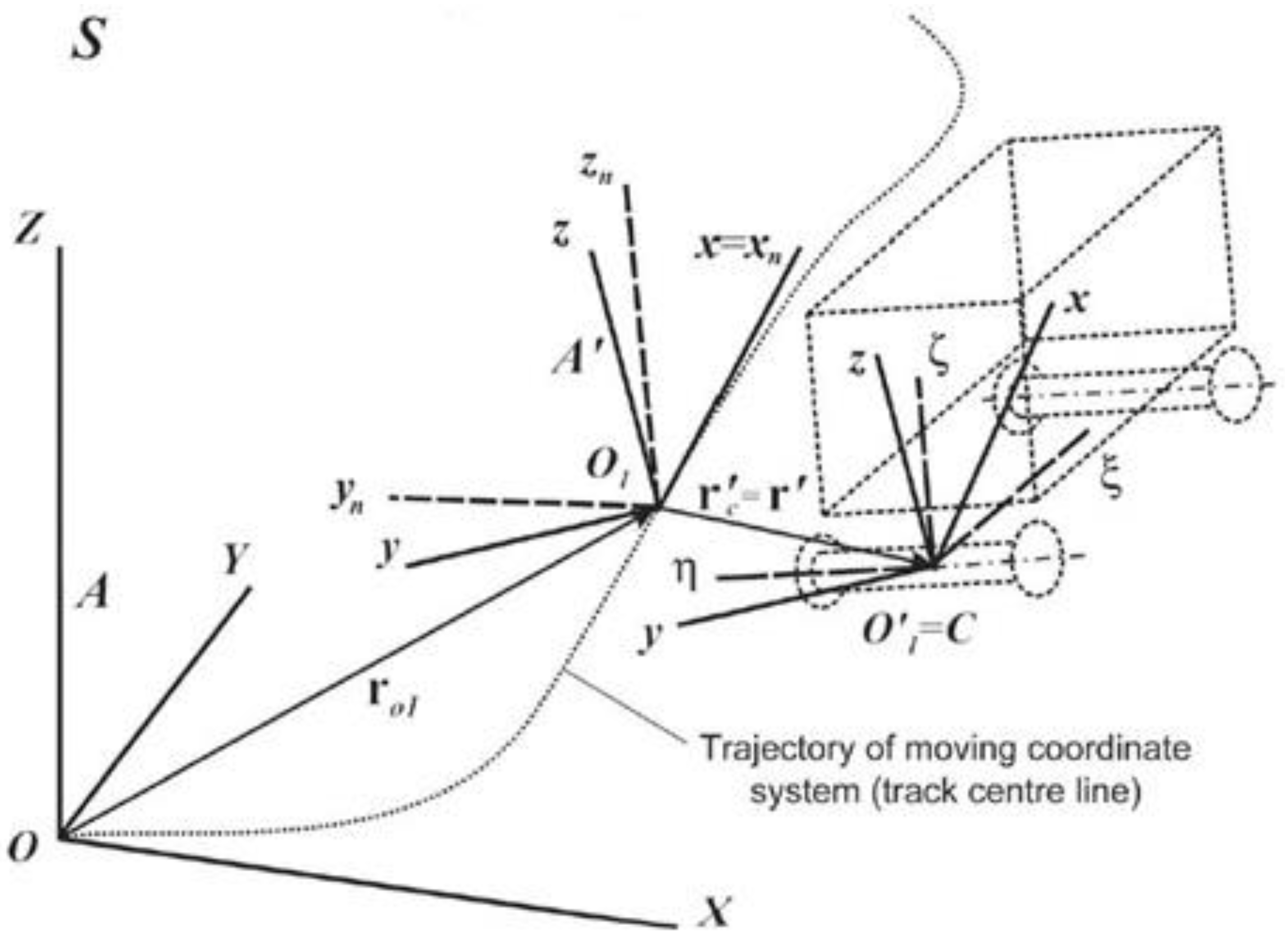
The approach to the shape modeling was widely defined [25]. Dynamics of relative motion is used in this method. The definition of vehicle dynamics is relative to the track-based moving reference frame (reference frame 01xyz at Figure 3). The idea applied in this work relied on the passage of rail model through the route (track) consisted in: Straight track, transition curve, and circular arc. The geometrical track model was generally analyzed in three dimensions.
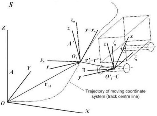
Figure 3.
Moving coordinate reference frame 01xyz.
It is also worthy of notice that in the current work, no track deformation—both lateral and vertical—caused by forces in the wheel/track contact is taken into account. The shape of the track is fixed and oriented in relation to the track center-line. The work has a theoretical character, and the analysis of track displacements is rather characteristic of works connected with railway maintenance.
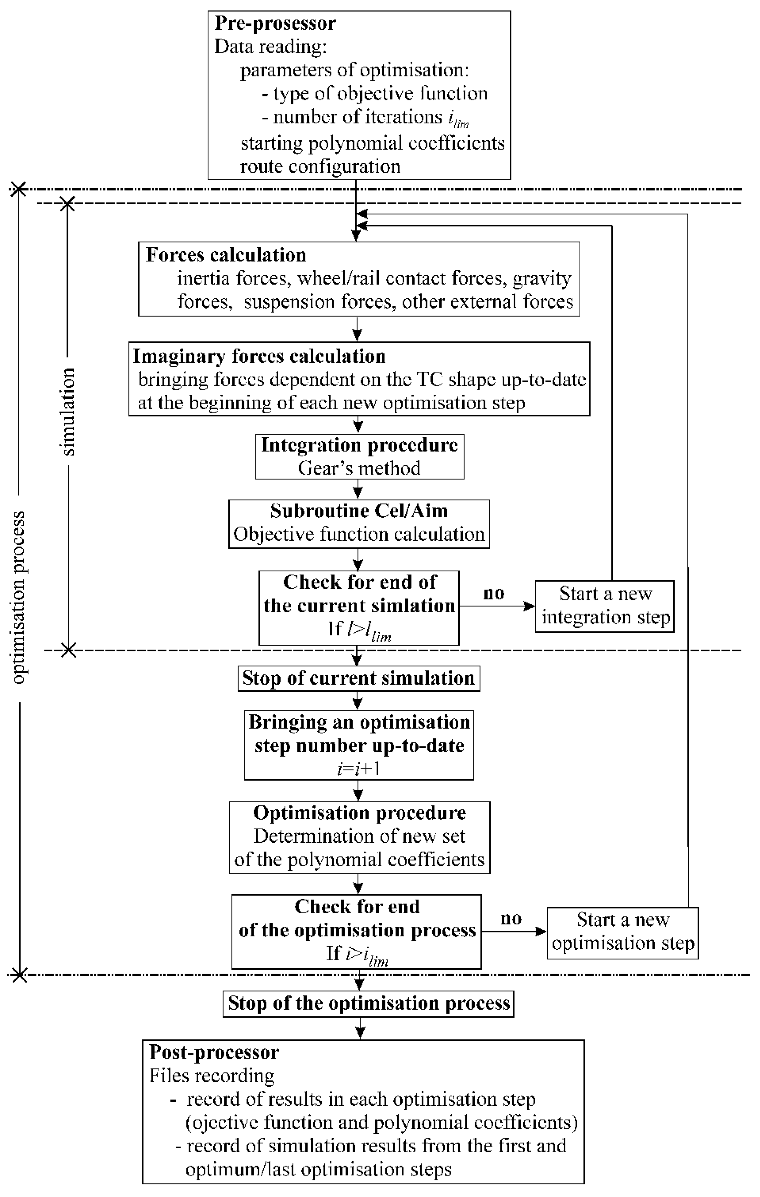
The scheme of the software is presented in Figure 4. There are two iteration loops. The first one is the integration loop. It stopped when the assumed length of the route is reached by the vehicle model. The second loop is the optimization process loop. This loop stopped when the limit assumed value of iteration is reached unless the optimum solution is not found earlier. In practice, 200 iterations were enough to find optimum solutions. The typical time of calculation was not greater than 1 h for each optimization, using Intel Core Duo 2 GB processor.
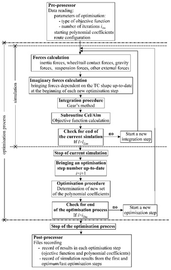
Figure 4.
The scheme of software.
4. Results of the Optimization
4.1. Results of the Optimization for 2-Axle Vehicle
This sectiom presents the general results of the optimization of railway transition curves performed by the authors of the current work. In the optimization made, the routes of the vehicle, as mentioned, were always composed of straight track, transition curve, and circular arc. Lengths of straight track were always the same and equal to 50 m. Similarly, the lengths of the circular arc were also the same and equal to 100 m.
In general, the optimization results are always comprised of: Optimum transition curves and their curvatures represented by the optimum polynomial coefficients, dynamics of the rail vehicle, mainly represented by displacements and acceleration of vehicle body and the wheelsets, and creepages in wheel-rail contact.
In Table 1, the authors presented parameters assumed in optimization for two different degrees of the polynomial—9th one and 11th one. These parameters are: The radius of circular arc R, the cant H, the length l0 of the curve, and vehicle velocity v. Admissible unbalanced acceleration alim on the track level was calculated for particular R, H, and velocity v, and ranged from −0.3 m/s2 (small velocities) to 0.6 m/s2.

Table 1.
Assumed parameters for 9th and 11th degrees.
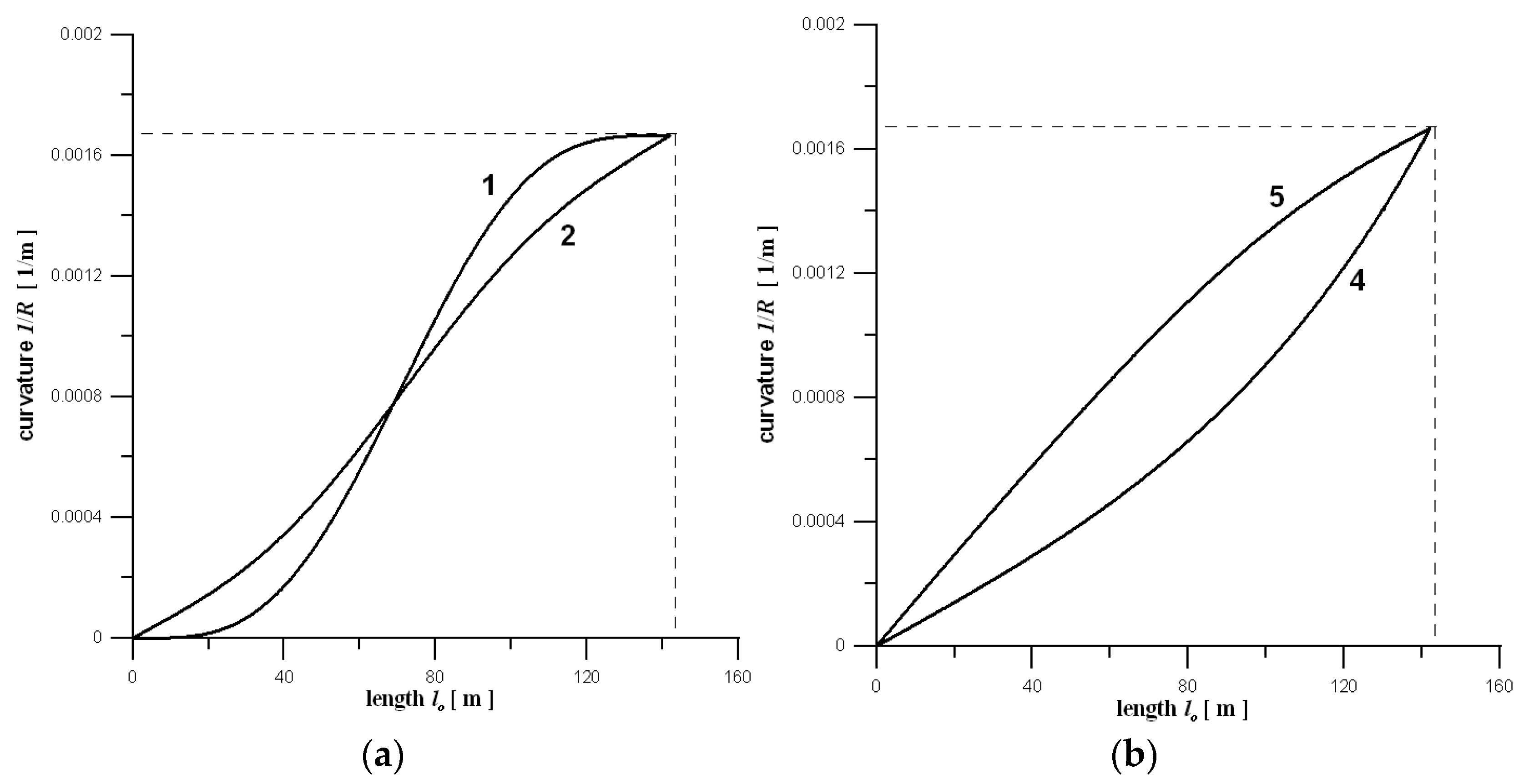
Generally, five typical shapes of the curves were obtained in this work. Their curvatures had one of the five possible shapes:
- 1
- The shape of the standard curve—type 1,
- 2
- The shape with the inflection point in the middle part of the curve—type 2,
- 3
- The linear shape as for the 3rd degree parabola—type 3,
- 4
- The convex shape on the route of the transition curve ([0, l0])—type 4,
- 5
- The concave shape on the route of the transition curve ([0, l0])—type 5.
Figure 5 presents four types of the curvatures—type no. 1, 2, 4, and 5.

Figure 5.
Types of curvatures: (a) 1 and 2; (b) 4 and 5.
In Table 2, the authors presented results for all 24 cases from Table 1, as represented by characteristic features of curvatures of the optimum transition curves shapes. Four cases from this table are taken as the representative ones to present the results of the optimization. For these cases, the single curve radius R and superelevation H for circular arc was assumed. Their values were R = 600 m and H = 0.15 m, respectively.
Table 2.
The results of the optimization for 9th and 11th degrees.
In all 24 analyzed cases from Table 2, the betterment of rail vehicle dynamics represented by smaller values of quality function was observed. New optimum transition curves improved all key dynamical characteristics of the vehicle, first of all—lateral displacement and acceleration of vehicle body. This fact can be crucial for journey passenger comfort.
Table 3 presents the values of optimum coefficients of the polynomial (Equation (1)) with accuracy to 5 decimal places for cases no. 2, 4, 14, and 16 from Table 2. In the rest of the work, it will be named the curves (2), (4), (14), and (16).
Table 3.
Optimum polynomial coefficients.
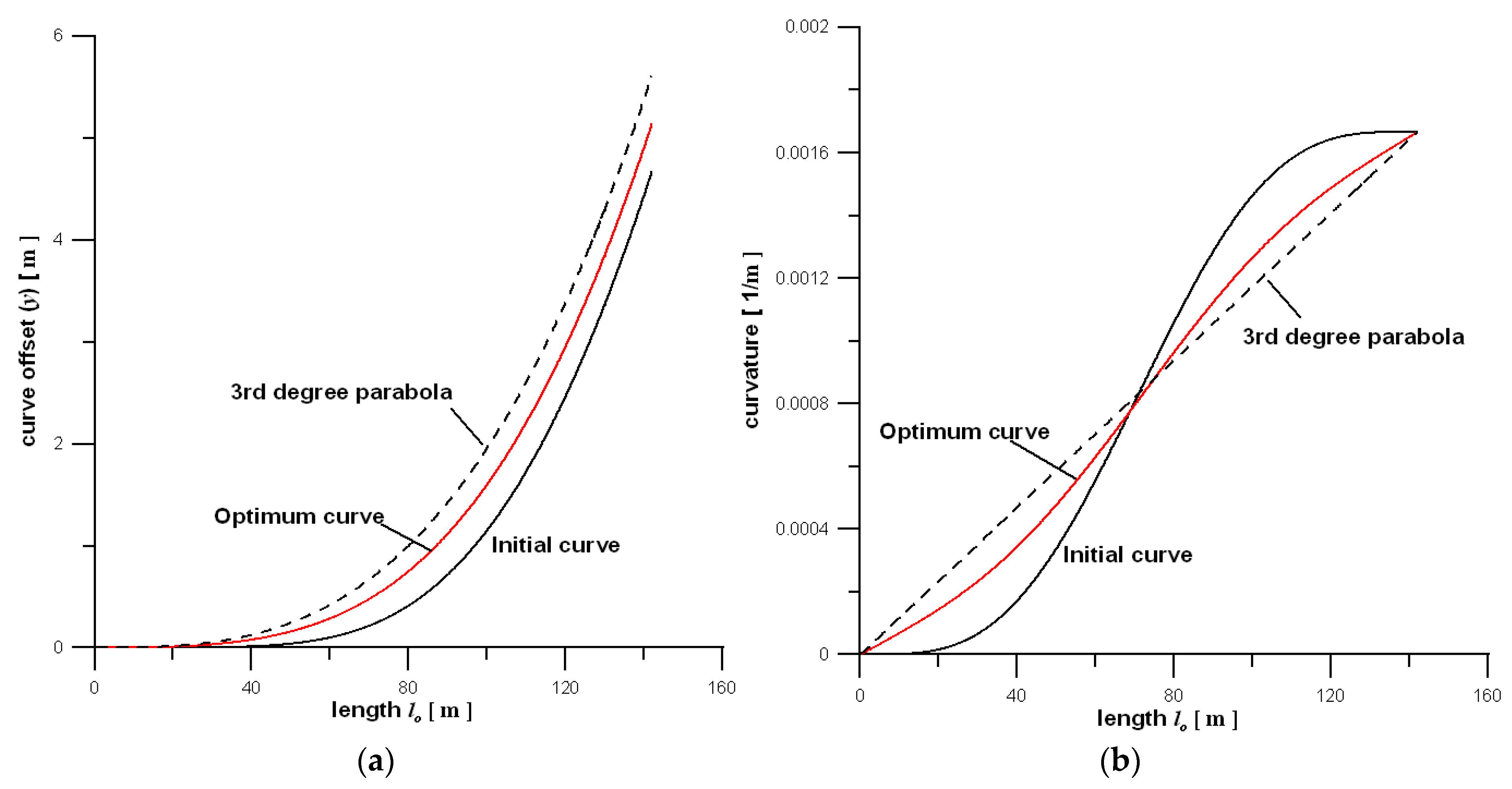
Graphical results are limited to the case no. 2 from Table 2. Figure 6a shows a comparison of transition curves (curve offsets y)—initial one (black line), optimum one (red line), and the 3rd degree parabola (dashed line), whereas Figure 6b shows their curvatures. It can be seen that both the offset, and the curvature of the optimum curve places it between the standard curve and the 3rd degree parabola. It is also visible that the curvature of the optimum curve is something between the standard curve and 3rd degree parabola.
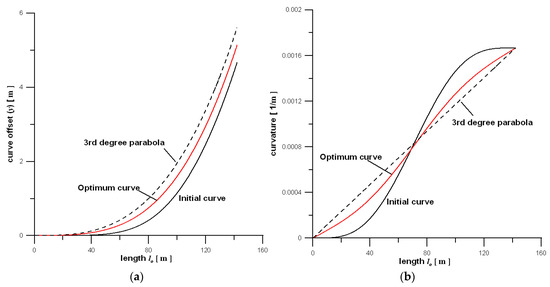
Figure 6.
Transitions curves: (a) Curve offsets; (b) curvatures.
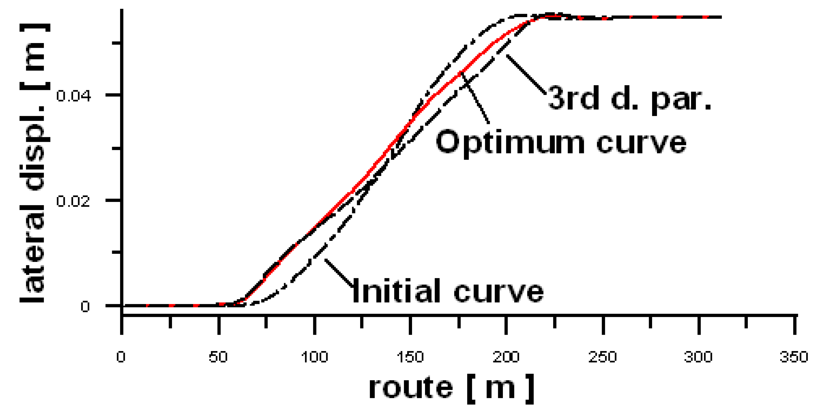
Figure 7 shows the comparison of the lateral displacement and acceleration of the center of mass of the car body for the initial curve, the optimum curve, and also the 3rd degree parabola. Both the displacement graph (Figure 7a) and the acceleration graph (Figure 7b) clearly show that the optimum curve is better than both the standard curve, and the 3rd degree parabola. Notably, in this context, interesting is Figure 7b for accelerations.
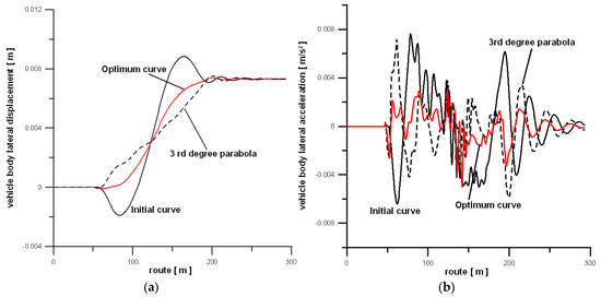
Figure 7.
Dynamical characteristics; (a) Vehicle body lateral displacements; (b) vehicle body lateral accelerations.
The ratio of the objective function values (the optimum curve/3rd degree parabola) is 0.59 = (0.0018622 [m/s2]/0.0031123 [m/s2]). The ratio of the optimum objective function value to that one for the 9th degree standard curve is 0.35 = (0.0018622 [m/s2]/0.0051947 [m/s2]).
Figure 8 presents the comparison of other graphical results—here, the lateral acceleration of the car body around the x-axis for the initial (standard) curve of 9th degree and the optimum curve. The betterment of rail vehicle dynamics is visible in comparison to the standard curve of 9th degree.
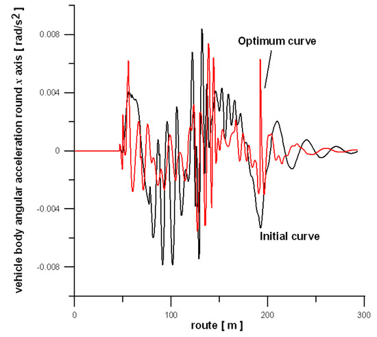
Figure 8.
Dynamical characteristics-vehicle body angular accelerations around x-axis.
4.2. Verification of Results of the Optimization with the Use of the 4-Axle Vehicle
The purpose of this sub-section is to show that the optimum transition curves 9th and 11th degrees presented in Section 4.1 maintain their positive properties, when a passenger vehicle (4-axle passenger car) is negotiating them. Recall that the shape optimization of the transition curves was optimized with a 2-axle vehicle with a much smaller number of degrees of freedom. It was dictated by shorter calculation times, and thus, a practical possibility of solving the task.
The analysis of the usefulness of the curves obtained for the needs of the previous section, and example, defined by coefficients (2), (4), (14), and (16) from Table 1 was performed with the ULYSSES program. The model of the four-axle MK-111 wagon, presented earlier in Section 2, was used here. The two variants of the second stage of the wagon suspension, i.e., the soft and the stiff variant, presented by the authors of [25] were used.
The aim of the simulations performed concerns the transition curves connecting with the circular arc. The parameters of arc were, as mentioned, R = 600 m and H = 0.15 m. The simulation data were identical to those used for determining the curves (2), (4), (14), and (16). The results concerned the vehicle’s travel along three curves:
- 1
- The 3rd degree parabola equal in length to the standard transition curve of 9th or 11th degree;
- 2
- The optimum curve for v = 24.26 m/s (respectively (2) for the 9th degree or (14) for the 11th degree) or the optimum curve for v = 30.79 m/s (respectively (4) for the 9th degree or (16) for the 11th degree);
- 3
- The standard curve for the 9th or 11th degree.
Eight cases were examined in the current work. The first two related to the movement of a vehicle with soft suspension along optimum curves of the 9th degree and different velocities, respectively v = 24.26 and 30.79 m/s. The next two cases concerned the movement of the vehicle with soft suspension along the 11th degree optimum curves with the same two speeds—v = 24.26 and 30.79 m/s. The next pair differed from the first one only in the use of a vehicle model with a stiff suspension. The last pair differed from the second pair again only in the use of the model with a stiff suspension. Two cases among the 8 analyzed (for the curves (2) and (14)) are presented in the figures in the further part of this section. The test results were limited to the presentation of the lateral displacements of the center of mass of the body of the tested model. Each of the presented figures contained the results for the three curves, thus, defined.
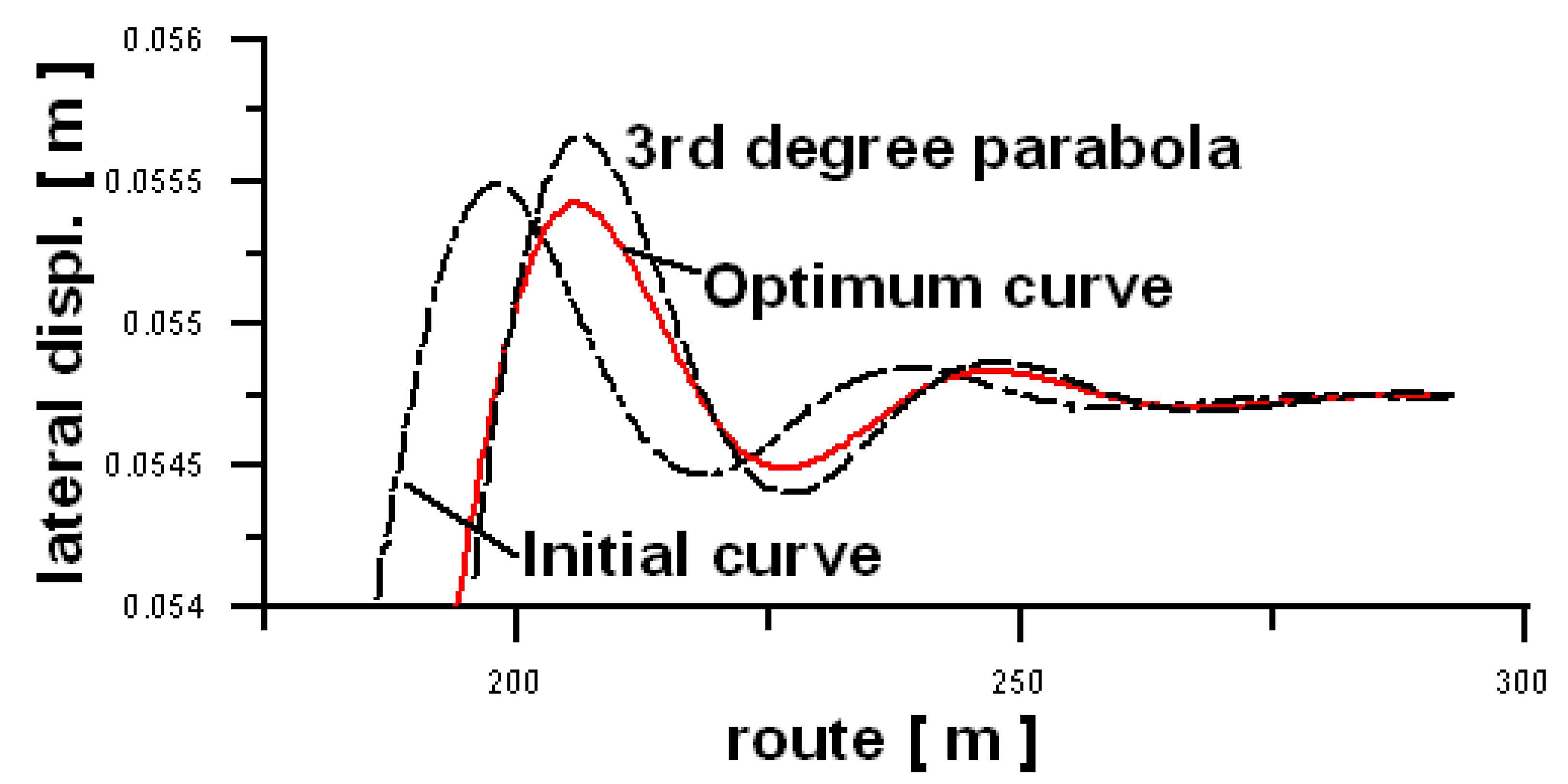
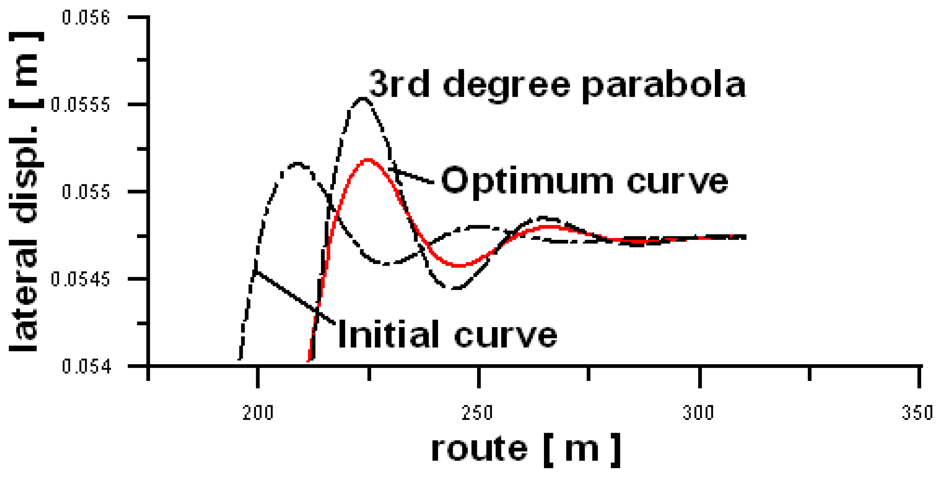
In the case of the vehicle with soft suspension and velocity v = 24.26 m/s, the optimum curves (2) and (14) showed features better than the 3rd degree parabola unequivocally for the considered length of the parabola, equal to the standard polynomial curve of 9th and 11th degree. This was proved by smoother transitions between them and the adjacent segments (straight track and circular arc) in Figure 9 and Figure 10, and a lower maximum value for the curves (2) and (14) than for the 3rd degree parabola in Figure 11 and Figure 12.
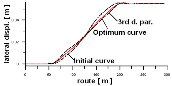
Figure 9.
Lateral displacements for 9th degree (soft suspension, v = 24.26 m/s2).

Figure 10.
Lateral displacements for 11th degree (soft suspension v = 24.26 m/s2).
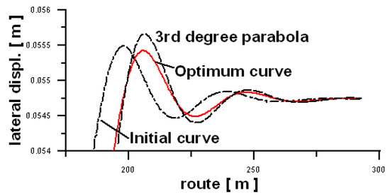
Figure 11.
Maximum displacements from Figure 9 under magnification.
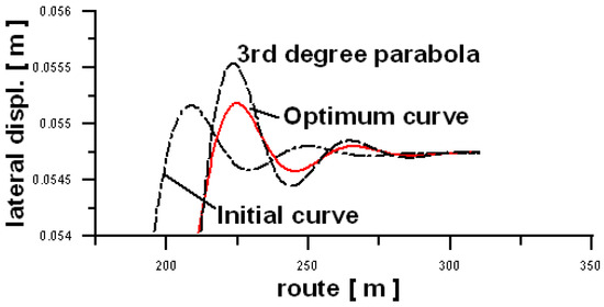
Figure 12.
Maximum displacements from Figure 10 under magnification.
In the six rest cases, four times the optimum curves had better properties than 3rd degree parabola, which was represented by the smaller maximum values of the lateral displacement of the 4-axle wagon. It was especially clear for the velocity of 24.26 m/s2.
5. Discussion
The presented method, using the 2-axle vehicle model and mathematically understood optimization, shows that it is possible to optimize the shape of the transition curve for a circular arc and cant. It is crucial from the perspective of designing railway infrastructure to reduce the negative impact of this infrastructure on the vehicle, and consequently, on the passenger.
The work showed that the new shapes of the transition curves obtained for a given circular arc result in milder dynamics represented mainly by displacements and accelerations of the vehicle body. The results obtained and presented in the current article constitute a certain novelty in the field of optimization and the properties assessment of railway polynomial transition curves. Obtained curves of 9th and 11th degrees had significantly better properties than what is known from the literature, as well as standard curves of those degrees and the 3rd degree parabola—the curve traditionally used. It is not disturbed by the fact that different circular arc radii generally resulted in different shapes of the curves. It has also been shown that these curves maintain their characteristics also for the 4-axle car model, which corresponds to a real passenger car. This confirms that the author’s efforts made sense. It also shows the correctness of the approach used in this work.
The results obtained during the research explain, why polynomial transition curves have not been used. The authors mean their small popularity. The curves of lower degrees are analyzed and used, and they do not satisfy the advanced boundary conditions (e.g., inclination function of bell-shaped). In the case of higher degrees, curves, more often analyzed than used, are expected to satisfy the advanced boundary conditions. Such an orientation to the lower degrees of the polynomial curves (without fulfilling advanced boundary conditions) can probably be treated as a mistake.
The obtained new shapes indicate the need for further study of the transition curves and set new directions for research. Note that although the equations of the obtained optimum curves have been defined, the obtained results can be viewed more broadly. Well, the obtained shapes indicate that it is worth taking a closer look at the transition curves connecting the features of the 3rd degree parabola and the well-known polynomial curves of higher degree, which we called the standard polynomial curves in this work. Note that such curves do not necessarily have to be polynomials. Perhaps it would be advantageous to use curve types that are even more flexible from the perspective of shape taking than polynomials. In this context, cubic splines (3rd degree spline curves) come to mind here.
The obtained results and the demonstration of the effectiveness of the approach used in this work allow the author to believe that the work is a good starting point for adopting new rules in the future and for constructing new methods of shaping transition curves. Methods, in which the core would be a combination of vehicle motion simulation methods and mathematical optimization methods. Efforts to change these principles and methods are likely to continue as long as no progress is made in this area. In this context, the author recognizes the contribution of this work to the discussion on this issue.
Author Contributions
Both authors (K.Z. and P.W.) equally contributed to the simulation, optimization, data analysis, and writing. All authors have read and agreed to the published version of the manuscript.
Funding
This research received no external funding.
Institutional Review Board Statement
Not applicable.
Informed Consent Statement
Not applicable.
Conflicts of Interest
The authors declare no conflict of interest.
References
- Zboinski, K. Dynamical investigation of railway vehicles on a curved track. Eur. J. Mech. A Solids 1998, 17, 1001–1020. [Google Scholar] [CrossRef]
- Zboinski, K. Numerical studies on railway vehicle response to transition curves with regard to their different shape. Arch. Civil. Eng. 1998, 44, 151–181. [Google Scholar]
- Bronshtein, I.; Semendyayev, K. Handbook of Mathematics; Springer: Berlin/Heidelberg, Germany, 2004. [Google Scholar]
- Klauder, L.T.; Chrismer, S.M. Improved spiral geometry for high-speed rail and predicted vehicle response. Rail Track Struct. 2003, 6, 15–17. [Google Scholar] [CrossRef]
- Li, X.; Li, M.; Ma, C.; Bu, J.; Zhu, L. Analysis on mechanical performances of high-speed railway transition curves. In Proceedings of the ICCTP 2009, Harbin, China, 5–9 August 2009; pp. 1–8. [Google Scholar]
- Lindahl, M. Track Geometry for High-Speed Railways; Department of Vehicle Engineering, Royal Institute of Technology: Stockholm, Sweden, 2001; p. 54. [Google Scholar]
- Vermeij, D. Design of a high speed track. HERON 2000, 45, 9–24. [Google Scholar]
- Xu, Y.L.; Wang, Z.L.; LI, G.Q.; Chen, S.; Yang, Y.B. High-speed running maglev trains interacting with elastic transitional viaducts. Eng. Struct. 2019, 183, 562–578. [Google Scholar] [CrossRef]
- Tari, E.; Baykal, O. A new transition curve with enhanced properties. Can. J. Civ. Eng. 2005, 32, 913–923. [Google Scholar] [CrossRef]
- Long, X.Y.; Wei, Q.C.; Zheng, F.Y. Dynamic analysis of railway transition curves. Proc. Inst. Mech. Eng. Part F J. Rail Rapid Transit 2010, 224, 1–14. [Google Scholar] [CrossRef]
- Eliou, N.; Kaliabetsos, G. A new, simple and accurate transition curve type, for use in road and railway alignment design. Eur. Trans. Res. Rev. 2014, 6, 171–179. [Google Scholar] [CrossRef] [Green Version]
- Kufver, B. Optimisation of Horizontal Alignments for Railway—Procedure Involving Evaluation of Dynamic Vehicle Response; Royal Institute of Technology: Stockholm, Sweden, 2000. [Google Scholar]
- Hasslinger, H. Measurement proof for the superiority of a new track alignment design element, the so-called “Viennese Curve”. ZEVrail 2005, 128, 61–71. [Google Scholar]
- Fischer, S. Comparison of railway track transition curves types. Pollack Period. 2009, 4, 99–110. [Google Scholar] [CrossRef]
- Kik, W. Comparison of the behaviour of different wheelset-trackmodels. Veh. Syst. Dyn. 1992, 20, 325–339. [Google Scholar] [CrossRef]
- Li, X.; Li, M.; Wang, H.; Bu, J.; Chen, M. Simulation on dynamic behaviour of railway transition curves. In Proceedings of the ICCTP 2010, Beijing, China, 4–8 August 2010; pp. 3349–3357. [Google Scholar]
- Li, X.; Li, M.; Bu, J.; Wang, H. Comparative analysis on the linetype mechanical performances of two railway transition curves. China Railw. Sci. 2009, 30, 1–6. [Google Scholar]
- Lian, S.L.; Liu, J.H.; Li, X.G.; Liu, W.X. Test verification of rationality of transition curve parameters of dedicated passenger traffic railway lines. J. China Rail. Soc. 2006, 28, 88–92. [Google Scholar]
- Michitsuji, Y.; Suda, Y. Improvement of curving performance with assist control on transition curve for single-axle dedicated passenger traffic railway lines. Jpn. Soc. Mech. Eng. 2005, 711, 107–113. [Google Scholar]
- Pirti, A.; Yucel, M.A.; Ocalan, T. Transrapid and the transition curve as sinusoid. Teh. Vjesn. 2016, 23, 315–320. [Google Scholar]
- Pombo, J.; Ambrosio, J. General spatial curve joint for rail guided vehicles: Kinematics and dynamics. Multibody Syst. Dyn. 2003, 9, 237–264. [Google Scholar] [CrossRef]
- Suda, Y.; Wang, W.; Komine, H.; Sato, Y.; Nakai, T.; Shimokawa, Y. Study on control of air suspension system for railway vehicle to prevent wheel load reduction at low-speed transition curve negotiation. Veh. Syst. Dyn. 2006, 44, 814–822. [Google Scholar] [CrossRef]
- Tanaka, Y. On the transition curve considering effect of variation of the train speed. ZAMM J. App. Math Mech. 2006, 15, 266–267. [Google Scholar] [CrossRef]
- Zhang, J.Q.; Huang, Y.H.; Li, F. Influence of transition curves on dynamics performance of railway vehicle. Jiaotong Yunshu Gongcheng Xuebao 2010, 10, 39–44. [Google Scholar]
- Zboinski, K.; Woznica, P. Optimisation of railway polynomial transition curves: A method and results. In Proceedings of the First International Conference on Railway Technology: Research, Development and Maintenance, Las Palmas de Gran Canaria, Spain, 18–20 April 2012; Civil-Comp Press: Stirlingshire, UK, 2012. [Google Scholar]
- Zboinski, K.; Woznica, P. Combined use of dynamical simulation and optimisation to form railway transition curves. Veh. Syst. Dyn. 2012, 56, 1394–1450. [Google Scholar] [CrossRef]
- Kobryn, A. New solutions for general transition curves. J. Surv. Eng. 2014, 140, 12–21. [Google Scholar] [CrossRef]
- Koc, W. New transition curve adapted to railway operational requirements. J. Surv. Eng. 2019, 145, 04019009. [Google Scholar] [CrossRef]
- Ahmad, A.; Ali, J. G3 transition curve between two straight lines. In Proceedings of the 2008 Fifth International Conference on Computer Graphics, Imaging and Visualisation, Penang, Malaysia, 26–28 August 2008; pp. 154–159. [Google Scholar]
- Ahmad, A.; Gobithasan, R.; Ali, J. G2 transition curve using quadratic Bezier curve. In Proceedings of the Computer Graphics, Imaging and Visualisation (CGIV 2007), Bangkok, Thailand, 14–17 August 2007; pp. 223–228. [Google Scholar]
- Barna, Z.; Kisgyorgy, L.J. Analysis of hyperbolic transition curve geometry. Period. Polytech. Civil. Eng. 2015, 59, 173–178. [Google Scholar] [CrossRef] [Green Version]
- Shen, T.-I.; Chang, C.H.; Chang, K.Y.; Lu, C.C. A numerical study of cubic parabolas on railway transition curves. J. Mar. Sci. Tech. 2013, 21, 191–197. [Google Scholar]
- CEN EN 12299:2009, Railway Applications—Ride Comfort for Passengers—Measurement and Evaluation; European Committee for Standardization: Brussels, Belgium, 2009.
- Esveld, C. Modern Railway Track; MRT-Productions: Zaltbommel, The Netherlands, 2001. [Google Scholar]


Publisher’s Note: MDPI stays neutral with regard to jurisdictional claims in published maps and institutional affiliations. |
© 2021 by the authors. Licensee MDPI, Basel, Switzerland. This article is an open access article distributed under the terms and conditions of the Creative Commons Attribution (CC BY) license (https://creativecommons.org/licenses/by/4.0/).