Modeling the Temperature Field in the Ground with an Installed Slinky-Coil Heat Exchanger

Abstract

In order to find the temperature field in the ground with a heat exchanger, it is necessary to determine temperature responses of the ground caused by heat sources and the influence of the environment. To determine the latter, a new model of heat transfer in the ground under natural conditions was developed. The heat flux of the evaporation of moisture from the ground was described by the relationship taking into account the annual amount of rainfall. The analytical solution for the equations of this model is presented. Under the conditions for which the calculations were performed, the following data were obtained: the average ground surface temperature T_sm = 10.67 °C, the ground surface temperature amplitude A_s = 13.88 K, and the phase angle P_s = 0.202 rad. This method makes it possible to easily determine the undisturbed ground temperature at any depth and at any time. This solution was used to find the temperature field in the ground with an installed slinky-coil heat exchanger that consisted of 63 coils. The results of calculations according to the presented model were compared with the results of measurements from the literature. The 3D model for the ground with an installed heat exchanger enables the analysis of the influence of miscellaneous parameters of the process of extracting or supplying heat from/to the ground on its temperature field.

1. Introduction

Among the many known types of heat exchangers, ground heat exchangers play an important role in installations with renewable energy sources. In recent years, there has been a significant development in terms of new designs and new ways of modeling and designing these devices. This progress is the result of numerous theoretical and experimental research studies on heat transfer between the working fluid flowing through the exchanger and the ground where the exchanger pipes are installed. Various ways of arranging the pipes of the ground heat exchangers, both horizontally and with vertical boreholes, have been developed. Recently, there have been attempts to use nanofluids as working fluids [1], like in the case of heat transfer between fluids [2]. Another modification involves the introduction of phase change materials with the ability to accumulate heat [3].

The ground heat exchangers are parts of the heat pump installations. The advantages of exchangers with horizontal pipes, compared to exchangers with vertical pipes, include lower investment costs and the use of the environment to supplement thermal deficiencies occurring in the ground (or to get rid of the excess heat).

Although many devices for monitoring the operation of ground heat exchangers have been installed in recent years around the world, few of them have been used to study the thermal behavior of the ground. Most of the measurement data relate to the obtained COP values. A small amount of data of temperature of the ground with an installed heat exchanger leads to an incomplete understanding of how the ground responds to extracting/supplying heat from/to a ground heat pump system.

Hepburn et al. [4] conducted studies on the ground temperature near a ground heat exchanger coupled with a heat pump. Their observations showed that most of the ground temperature changes near the heat exchanger pipes were caused by the variable temperature of the ground surface, and not by the heat extraction.

In the work by Wu et al. [5], measurements of the temperature of the ground near a slinky-coil heat exchanger coupled with a heat pump for space heating were presented. The horizontal spiral coils of the exchanger pipes were arranged in four rows, each one was 1 m wide and 80 m long, they were placed at a depth of 1.14 m.

Pauli et al. [6] monitored the ground temperature with installed horizontal ground heat exchangers of various configurations. The research concerned the collection of heat from the ground. The conclusions from the research were qualitative: (a) the ground temperatures rarely dropped below zero during most of the heating season, (b) the lowest temperatures occurred near the ground surface and not at the level of the heat exchanger installation, and (c) only at the end of the heating season did the ground temperature drop below the ambient temperature.

Neuberger and Adamovsky [7,8] conducted measurements of the ground temperature near the slinky-coil and straight pipe exchangers. The research was conducted both during the heating season and for the thermal regeneration of the ground. It was found that, in contrast to the exchanger with straight pipes, the ground temperature near the slinky-coil exchanger dropped below 0 °C during the heating season.

Jeon [9] compared the operation of the slinky-coil and straight pipe exchangers using the concept of a scale factor that was defined as the ratio of the mean thermal energy transferred for the spiral-coil-type GHE to that for the straight-line-type GHE.

The results of ground temperature measurements near the ground heat exchangers are often not confronted with appropriate mathematical models of heat transfer processes. Therefore, an attempt was made to create such a model.

The superposition principle [10] is the basis for modeling heat transfer in the ground with an installed heat exchanger. The complicated heat transfer process in the pipe system is composed of two independent elementary heat transfer processes. The first one is the heat transfer between the source (the surface of the pipes) and the semi-infinite medium (ground) with an isothermal boundary. The second process is the transfer of heat in this medium with a changing temperature on its surface. Therefore, to calculate the temperature of the ground, the temperature responses of the ground due to heat sources ϑ and the temperature responses of the varying temperature of the ground surface ϑ₀ must be taken into account:

T = T_init + ϑ + ϑ₀

In the absence of heat sources, i.e., for ϑ = 0, the ground temperature is T₀ = T_init + ϑ₀, and therefore:

T = T₀ + ϑ,

(1)

In designing and modeling of the ground heat exchangers, it is necessary to know the ground temperature field T₀ under natural conditions, i.e., in the ground without a heat exchanger installed. The temperature under these conditions varies with time and location and is called the undisturbed ground temperature (the same name is also used for the ground temperature at great depths; however, in this work, the undisturbed ground temperature should be understood as the temperature previously described).

The solution of the heat conduction equation for a semi-infinite body with periodic changes of its surface temperature is known (Carslaw and Jaeger [10]):

$$T_0=T_{sm}-A_s·\exp \left(-\frac{z}{L}\right)·\cos \left(\omega t-P_s-\frac{z}{L}\right),$$

(2)

The results of extensive studies on the ground temperature at various depths under different climatic conditions in the USA were presented by Kusuda and Achenbach [11]. Based on the measurement results, the coefficients of Equation (2) were determined and the results were in good agreement with the model.

This paper presents a new model of heat transfer in the ground under natural conditions. The heat flux for the evaporation of moisture from the ground was described with a linearized relationship taking into account the annual amount of rainfall. The analytical solution of the model equations enables users to easily determine the parameters of Equation (2): T_sm, A_s, P_s, and hence the undisturbed ground temperature profile. The profile was used to find the temperature field in the ground with an installed slinky-coil exchanger. When determining the ground temperature field, the intermediate results of calculations of ground temperature responses $\vartheta$ and undisturbed ground temperature T₀ were used to compare their time courses.

The aim of this work was to present and implement a model describing the temperature field for the ground in which a slinky-coil exchanger is placed. The simulation concerned the climatic conditions for East-Central Europe. Moreover, the results of calculations according to the presented model were compared with the results of measurements from the literature.

The model for the ground with an installed heat exchanger enables the analysis of the influence of various parameters of the process of extracting or supplying heat from/to the ground on its temperature field. The knowledge of the temperature field near the ground heat exchanger is important for the intensive extraction or supply of heat from/to the ground. Both excessive cooling and excessive ground overheating are unfavorable for the further operation of the exchanger.

2. Heat Fluxes on the Ground Surface

The following heat fluxes occur on the ground surface: convective flux, radiant flux, moisture evaporation flux, and conductive flux.

2.1. Convective Flux

The convective flux can be described by the heat transfer equation:

$$H=h\left(T_a-T_s\right),$$

(3)

The average daily values of air temperature and ground surface temperature change with time according to the following dependencies:

$$T_a=T_{am}-A_a\cos \left(\omega t-P_a\right),$$

(4)

$$T_s=T_{sm}-A_s\cos \left(\omega t-P_s\right),$$

(5)

The heat transfer coefficient between the ground surface and the surroundings, h, depends on the wind speed at the ground surface and the type of ground surface covering. Among the many empirical relationships from the literature, the following formula is often used to determine the h coefficient:

$$h=\frac{{\rho }_a{c}_{pa}}{r_a},$$

(6)

where ρ_a and c_pa are the density and heat capacity of air, and r_a is the aerodynamic resistance to heat transfer. For example, when the ground is covered with 0.12 m high plants, the following dependency can be used [12]:

$$r_a=\frac{208}{u},$$

(7)

where u is the wind velocity 2 m above the ground.

2.2. Radiant Flux

The average daily solar radiation (short-wave) flux absorbed by the ground changes in the annual cycle according to the relationship:

$$S=S_m-A_{sol}\cos \left(\omega t-P_{sol}\right),$$

(8)

The long-wave radiation flux refers to the transport of heat from the ground surface to the sky (Earth radiation). Since the surface temperature of the ground T_s is higher than the temperature of the sky T_sky, the ground radiates thermal energy. Due to the low temperature of the radiation source, it is the long-wave type radiation. The average daily net flux LW of the long-wave radiation is:

$$LW=\epsilon \sigma \left(T_s^4-T_{sky}^4\right),$$

(9)

The relationship (9) was transformed into the linear form with respect to the temperature of the ground surface [13]. Since:

$$d\left({\xi }^4\right)=4{\xi }^{3}d\xi ,$$

Therefore:

$$T_s^4-T_{sky}^4\cong 4T_m^3\left(T_s-T_{sky}\right),$$

(10)

where T_m is the mean from the interval (T_sky, T_s). Thus, the average daily long-wave radiation flux is:

$$LW\cong \epsilon C_{LW}\left(T_s-T_{sky}\right),$$

(11)

where:

$$C_{LW}=4\sigma T_m^3,$$

(12)

Figure 1 shows the relationship between the expressions on the right-hand sides of Equations (9) and (11). For the T_s − T_sky interval between 10 and 20 K and the value of T_s ≈ 10 °C, the relationship was approximated by the linear equation (coefficient of determination R² = 0.99975, standard deviation σ = 0.20 × 10⁸ K⁴). On the basis of the coefficient of this equation, the value of T_m in Formula (10) was determined: T_m = 275.1 K and the value of the constant C_LW was found C_LW = 4.72 W/(m²K).

The temperature of the sky T_sky is related to the air temperature by the relationship resulting from the Stefan–Boltzmann equation [14,15]:

$$T_{sky}={\epsilon }_{sky}^{0.25}{T}_a,$$

(13)

where T_sky and T_a are expressed in [K] and ε_sky is the effective emissivity of the sky. In order to determine ε_sky, the results of the measurements presented in the work by Bryś et al. were used [16], which showed that the average annual net long-wave radiation flux is LW = 45.7 W/m². This value applies to the ground surface not covered with plant under the conditions of the measurements (Wrocław, Poland).

For calculations, the average annual air temperature and the average annual temperature of the ground surface under similar climatic conditions were adopted: T_am = 8.95 °C [17] and T_sm ≈ 10° C. The unit emissivity of the ground surface was assumed and the annual average temperature of the sky was calculated from Formula (9): T_sky,m = 273.5 K, and the effective emissivity of the sky—according to Formula (13): ε_sky = 0.893.

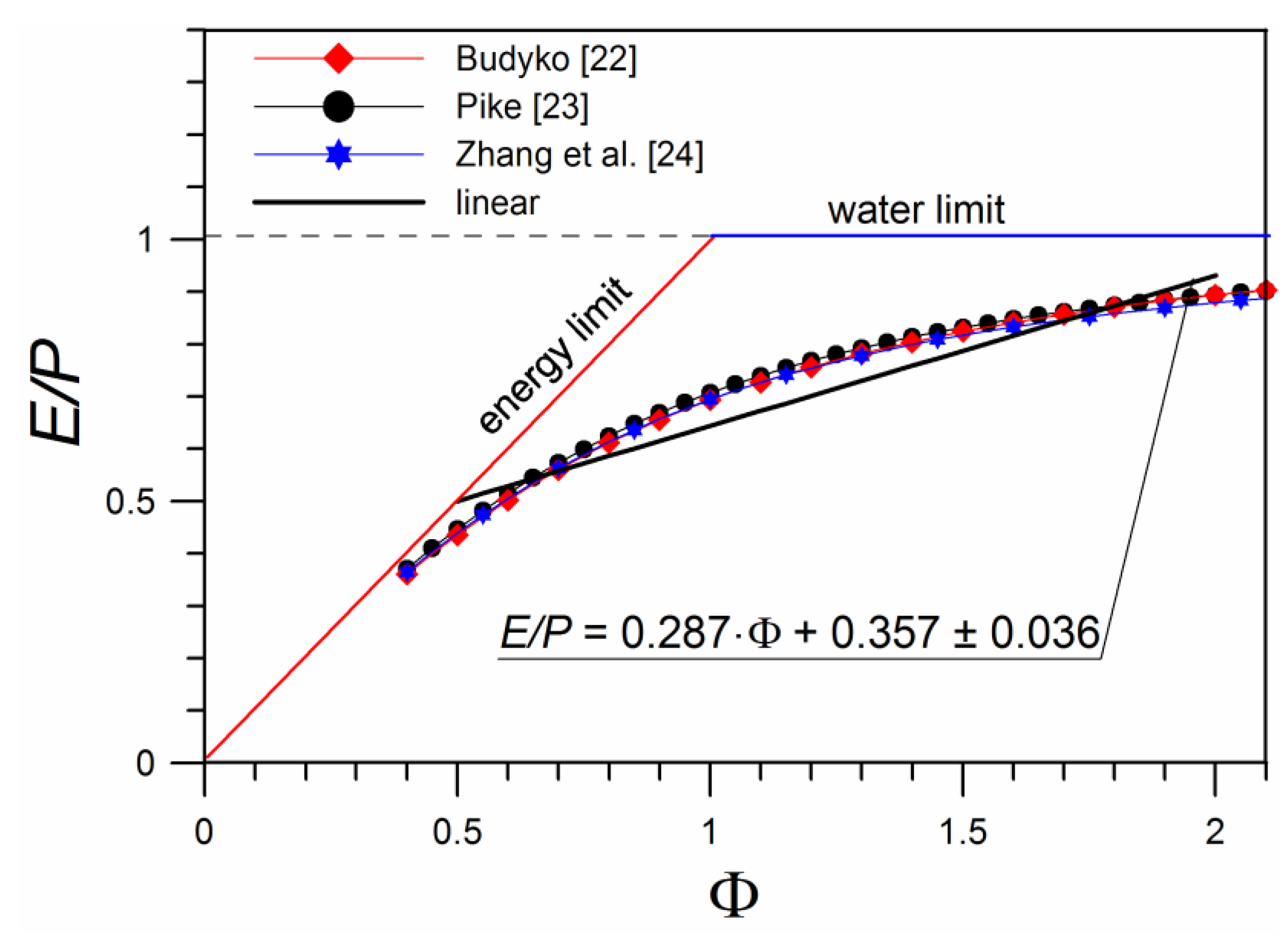
2.3. Evaporative Flux

Heat is also transferred between the ground surface and its surroundings as a result of the evaporation of water contained in the ground. Convective transfer coefficients are related to each other by the Chilton-Colburn heat and mass transfer analogy [18]. The resulting Penman-Monteith equation [19,20] determines the potential of the evaporated water stream:

$$E_0=\frac{1}{L_{evap}}·\frac{\Delta ·\left(S-LW\right)+{\rho }_a{c}_{pa}\left(p_{sat,s}-p\right)/r_a}{\Delta +{\gamma }_0\left(1+r_c/r_a\right)},$$

(14)

where Δ = dp_sat/dT, γ₀ (= 59.5 Pa/K)—psychrometric constant, r_c—crop canopy resistance, p_sat,s and p—partial pressures of water vapor on the ground surface and in the atmospheric air, respectively.

Equation (14) relates to the potentially possible rate of water evaporation from the ground. The actual evaporation rate E may be lower than E₀ due to the lack of moisture in the ground. To estimate the actual rate of evaporation, the inflow of water to the ground, mainly determined by the annual rainfall P, should be taken into account. Therefore, the relationship between the aridity index Φ = E₀/P and the E/P ratio is considered, i.e., the Budyko curve [21,22,23,24]. For Φ < 1 the evaporation rate is limited by E₀ (i.e., by the energy supply), while for Φ > 1 the evaporation rate is limited by the available amount of water P. Pike [23] proposed the following empirical relationship:

$$\frac{E}{P}=\frac{1}{\sqrt{1+{\left(1/\Phi \right)}^2}},$$

(15)

It should be noted that most of the experimental studies on which the Budyko curve is based concerned the range 0.5 < Φ < 2.0 and showed a significant dispersion. Figure 2 shows the approximations of the Budyko curve according to the research of various authors. The relationship (15) was approximated by a straight line for the range of Φ from 0.5 to 2, and then transformed to the form:

$$E=C_1{E}_0+C_{2}P,$$

(16)

where C₁ = 0.287 and C₂ = 0.357. From this dependence, it can be seen what share in the actual flux of the evaporated water has the evaporation potential E₀ and the annual amount of precipitation P.

In order to express the heat flux for water evaporation in a linear form with respect to the temperature of the ground surface, the dependence between the saturated water vapor pressure and temperature was approximated with a linear equation [25] (p_sat [Pa], T [°C]):

$$p_{sat}=a_{P}T+b_P,$$

(17)

where a_P = 103 Pa/K, b_P = 609 Pa. Taking into account dependencies (14), (16), and (17) and that EV = L_evap·E, one can obtain the expression for the evaporative heat flux:

$$EV=\beta h\left[\left(T_s+b_P/a_P\right)-RH\left(T_a+b_P/a_P\right)\right]+\beta \left(S-LW\right)+C_2{L}_{evap}P,$$

(18)

where:

$$\beta =\frac{C_1{a}_P}{a_P+{\gamma }_0\left(1+r_c/r_a\right)},$$

(19)

Expression (18) consists of three components. The first is the result of the mass transfer driving force, i.e., the difference in partial pressures of water vapor on the ground surface and in the bulk of the gas phase. The second component depends on the heat supplied to the system externally (from radiation). The third component takes into account the effect of the amount of water supplied to the system in the form of rainfall. The significance of the latter effect was demonstrated by the authors in [26] by formulating an empirical equation. Figure 3 shows the effect of the average annual solar radiation flux S_m and the annual precipitation P on the time courses of the evaporative heat flux EV. The increase in the intensity of solar radiation, as well as the increase in the amount of precipitation, causes the evaporative heat flux to increase. The maximum value of the evaporative flux EV occurs in the period of the year close to the period with the maximum temperature of the ground surface.

2.4. Thermal Balance on Ground Surface—The Analytical Solution

The heat flux q_cond resulting from the algebraic summation of the above-mentioned fluxes is transported (as a conductivity flux) deep into the ground or in the opposite direction depending on the sign. With the use of the average daily values, the heat balance on the ground surface can be written as follows [13,25,26,27,28,29]:

$$q_{cond}=H-LW+S-EV,$$

(20)

On the other hand, the balance equation for the average annual fluxes has the form:

$$q_{cond,m}=H_m-{\left(LW\right)}_m+S_m-{\left(EV\right)}_m,$$

(21)

Under natural conditions, the ground is in a cyclic steady state, and therefore the average annual conductivity flux is zero:

$$q_{cond,m}=0,$$

(22)

On the basis of the relationships for the individual heat fluxes, presented in Section 2.1, Section 2.2 and Section 2.3, the average annual fluxes H_m, (LW)_m, and (EV)_m can be expressed as a function of the average annual temperature of the ground surface T_sm, and hence after the substitution to Equation (21), one can determine this temperature:

$$T_{sm}=\frac{r_2{T}_{am}+\left(1-\beta \right)S_m-r_3}{r_1},$$

(23)

where:

$$r_1=h\left(1+\beta \right)+C_{LW}\left(1-\beta \right),$$

(24)

$$r_2=h\left(1+\beta ·RH\right)+C_{LW}{\epsilon }_{sky}^{0.25}\left(1-\beta \right),$$

(25)

$$r_3=\frac{\beta h{b}_P}{a_P}\left(1-RH\right)+C_2{L}_{evap}P+273.15·C_{LW}\left(1-{\epsilon }_{sky}^{0.25}\right)\left(1-\beta \right),$$

(26)

The values of the amplitude A_s and the phase shift P_s of the ground surface temperature can be determined on the basis of the balance of average daily fluxes (20). For the conductivity flux, it should be substituted in accordance with the Fourier equation:

$$q_{cond}=-k{\left(\frac{\partial T}{\partial z}\right)}_{z=0},$$

(27)

The phase shift and amplitude are determined by the formulas:

$$P_s={\tan }^{-1}\frac{p_1+p_2\left(1+p_3\right)}{p_1\left(1+p_3\right)-p_2},$$

(28)

$$A_s=\frac{p_3}{1+p_3}\left(p_1\cos P_s+p_2\sin P_s\right),$$

(29)

where:

$$p_1=\frac{A_a{r}_2\cos P_a+A_{sol}\left(1-\beta \right)\cos P_{sol}}{r_1},$$

(30)

$$p_2=\frac{A_a{r}_2\sin P_a+A_{sol}\left(1-\beta \right)\sin P_{sol}}{r_1},$$

(31)

$$p_3=\frac{r_{1}L}{k},$$

(32)

The derivation of dependencies (28) and (29) was discussed in [13,29].

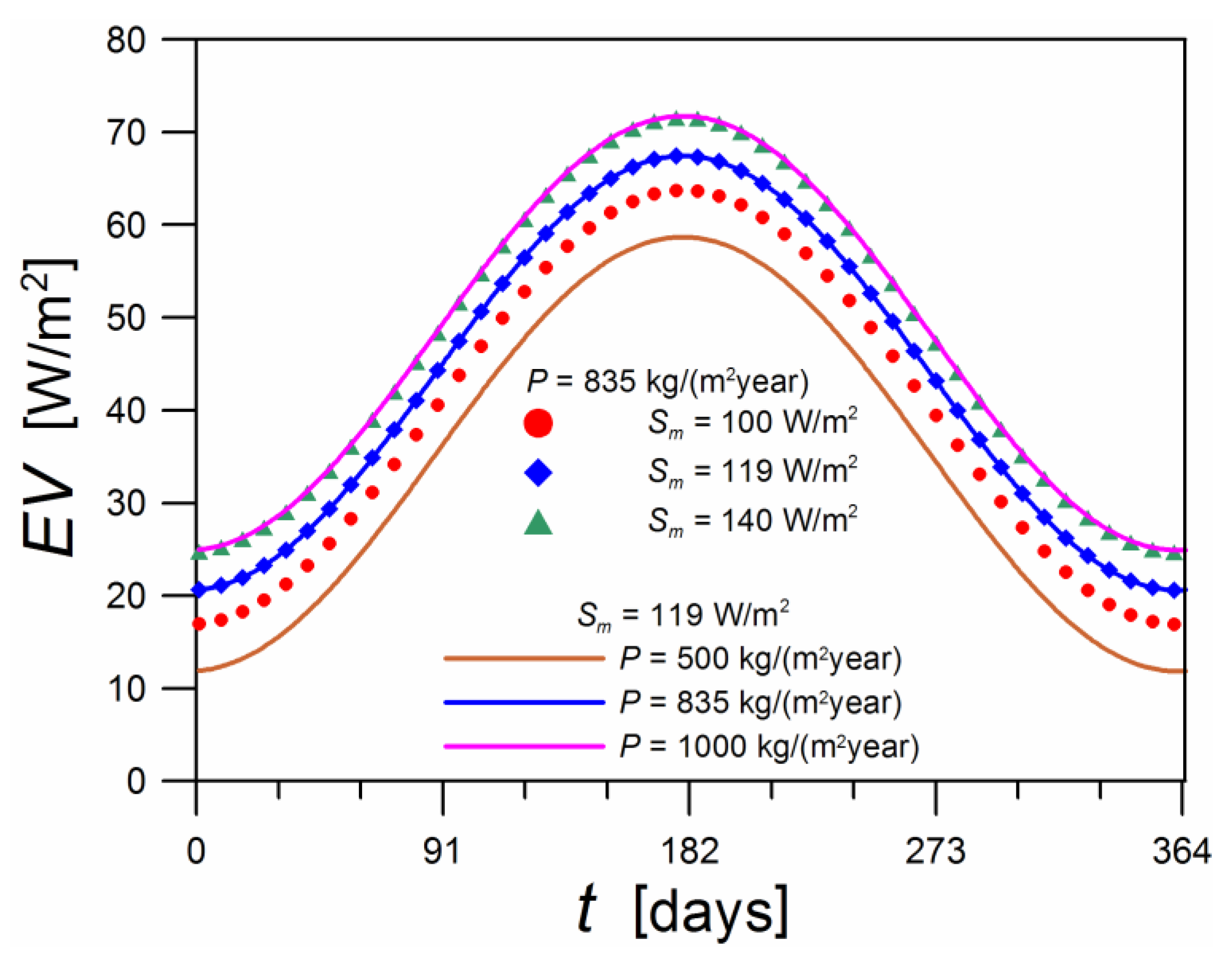
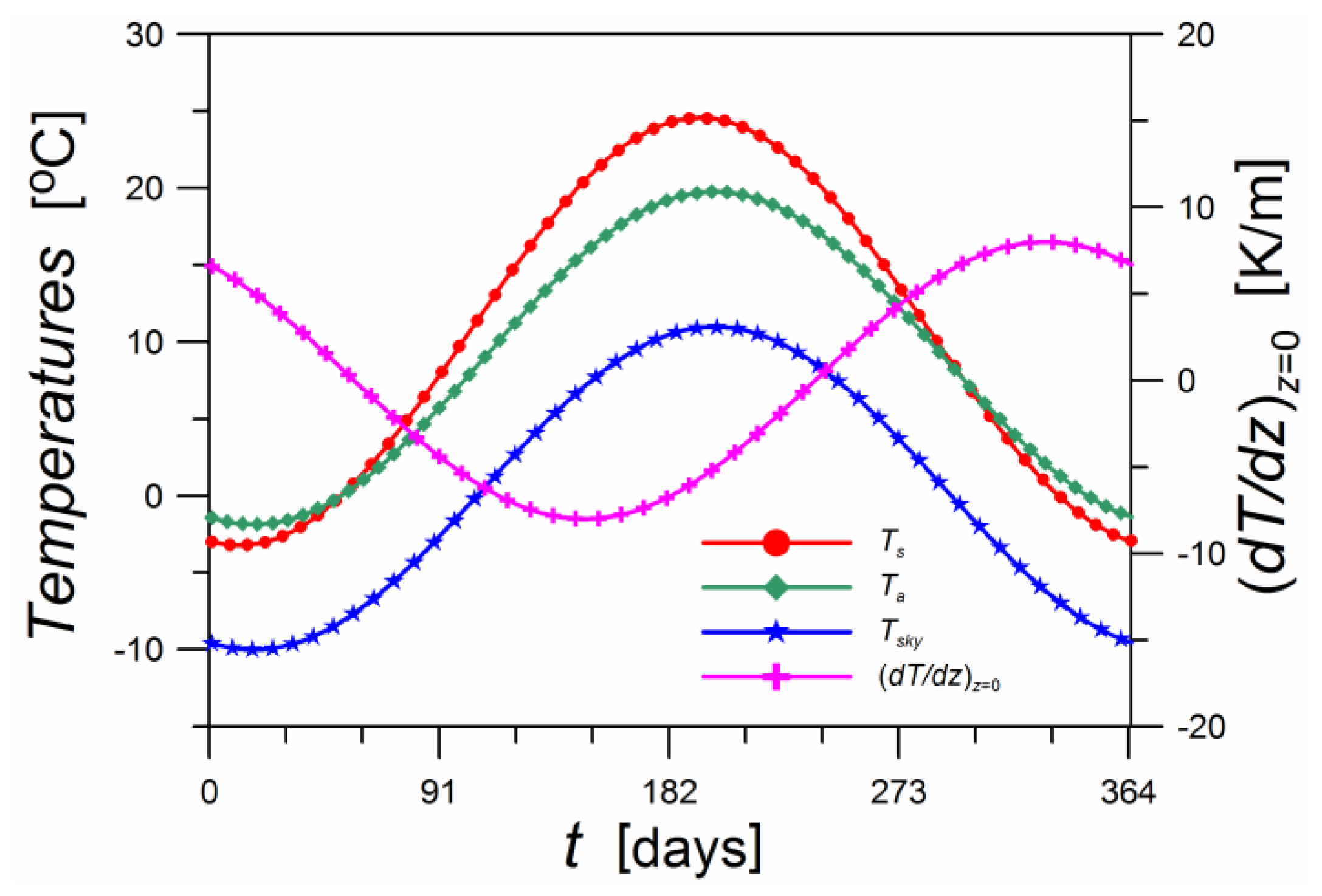
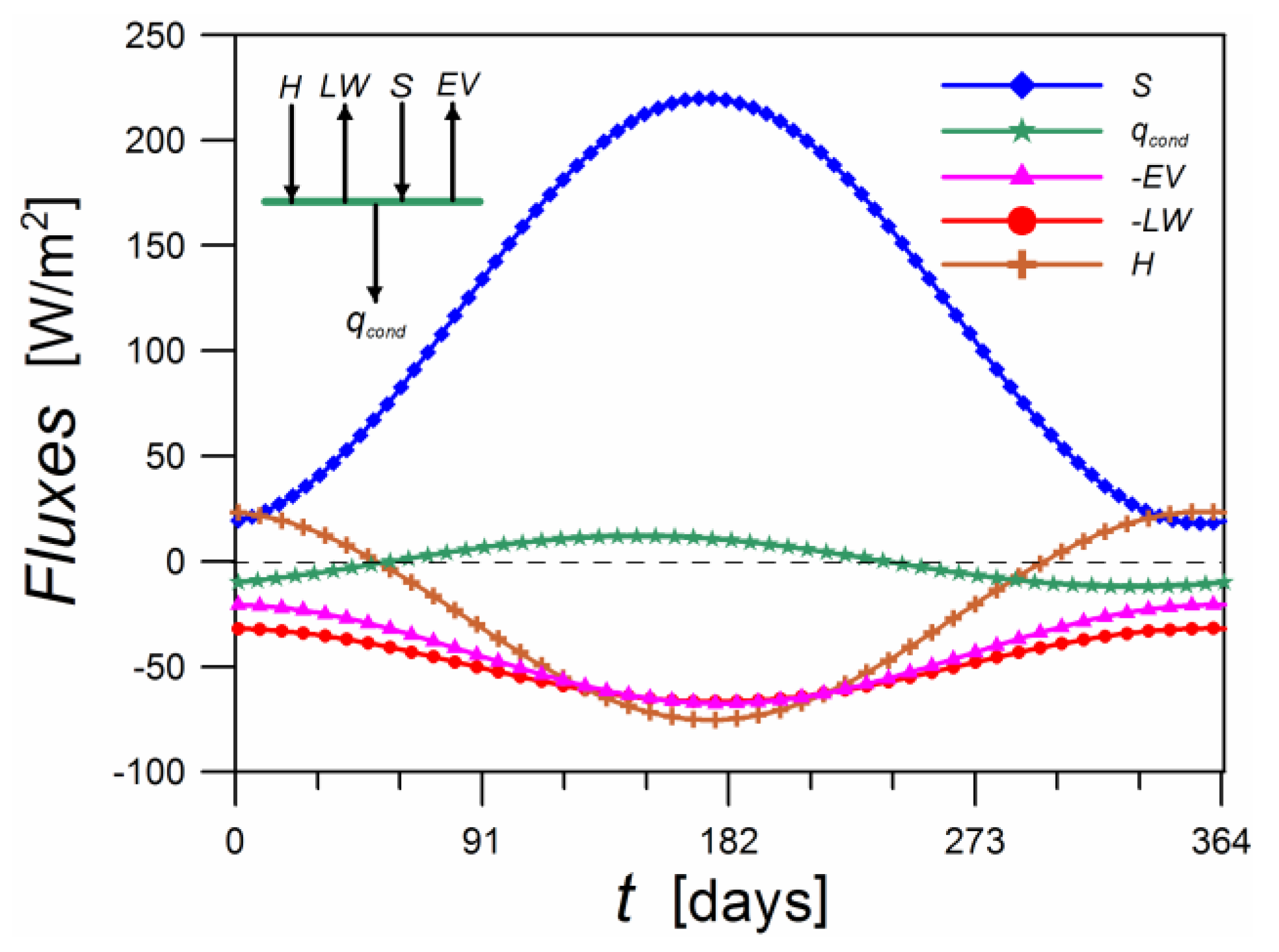
2.5. Examples of Time Courses of Heat Fluxes on the Ground Surface and Temperatures

The values presented in

Table 1. Numerical values used for calculating the temperature field under natural conditions.

Quantity	Value	Quantity	Value
Tam	8.95 °C	RH	0.758
Aa	10.81 K	k	1.50 W/(mK)
Pa	0.300 rad	α	0.6 × 10−6 m2/s
Sm	119 W/m2	Levap	2.47 × 106 J/kg
Asol	101 W/m2	rc	70 s/m
Psol	−0.153 rad	u	2.56 m/s
P	835 kg/(m2year)	L	2.45 m

were taken for calculations.

From dependencies (23), (28), and (29) the following parameters of Equation (2) were obtained: T_sm = 10.67 °C, A_s = 13.88 K, P_s = 0.202 rad. The coefficient r_a was calculated according to Formula (7), for which the value from Table 1 was used as the wind speed. The time courses of temperatures are shown in Figure 4, while the courses of individual heat fluxes are presented in Figure 5.

For most of the year, the temperature of the ground surface is higher than the air temperature. Moreover, the temperature of the ground surface has a greater amplitude than the air temperature. The temperature of the sky (daily average) is lower than the air temperature and the temperature of the ground surface. The ground surface temperature gradient is negative in the summer months, and positive in the winter months.

The solar radiation flux is always directed towards the ground surface. On the other hand, the long-wave and evaporative (daily average) radiation fluxes are directed in the opposite direction. The average value of the long-wave radiation flux is about 50 W/m². The convective and conductive fluxes change their direction twice a year; the convective flux causes heat losses through the ground throughout the year, while the average annual conductivity flux is zero. The Fourier equation relates the course of the conductivity flux with the temporal course of the temperature gradient on the ground surface.

3. Ground Temperature Field with an Installed Heat Exchanger

3.1. The Heat Flux Extracted from the Ground

In order to simulate the heat transfer in the ground with an installed heat exchanger, the time dependence of the heat flux taken from the ground should be known. A simplified model was adopted in which it was assumed that:

• Heat is extracted from the ground only for space heating purposes.
• Outside the heating season, no heat is supplied to the ground.
• The average daily value of the heat flux extracted from the ground q_GHE is assigned to each day of the year.
• The maximum value of the heat flux extracted from the ground is q_max.
• The number of days in the year h_d for which heat is extracted from the ground for heating purposes is known; for the remaining days, q_GHE = 0.

With such assumptions, the heat flux extracted from the ground, q_GHE, varies with time according to the relationship [29]:

$$q_{GHE}=\frac{q_{max}\left(\chi +\left|\chi \right|\right)}{2},$$

(33)

where:

$$\chi =\frac{\cos \left(\omega t-P_a\right)+a}{1+a},$$

(34)

$$a=-\cos \left(\pi \frac{h_d}{365}\right),$$

(35)

Figure 6 shows the annual course of the heat flux extracted from the ground for different values of h_d, in accordance with dependencies (33)–(35). Integrating the dependence of q_GHE on t, in the range corresponding to the heating season, allows one to determine the amount of heat Q extracted from 1 m² of the ground during the year.

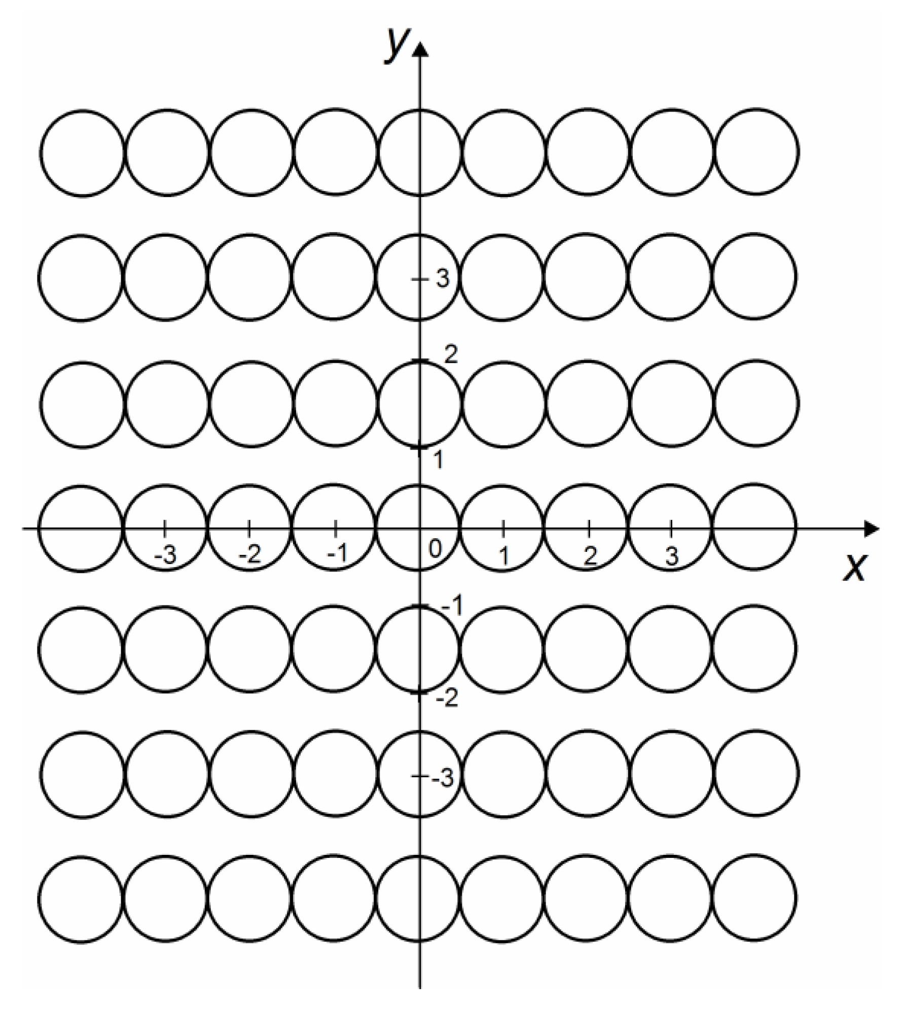
3.2. Application of the Ring Heat Source Model

It was assumed that the thermal power of each ring as a heat source is the same. This power is determined by the relationship:

$${\dot{Q}}_{extr,j}=-q_{GHE}{A}_j,$$

(36)

where A_j is the ground area per ring. The ground temperature response at time t at the point P with coordinates x, y, and z, caused by the action of N_ring ring heat sources, was determined according to the equation [30,31]:

$$\vartheta =\frac{1}{8c_v{\left(\pi \alpha \right)}^{3/2}}{{\displaystyle \sum }}_{j=1}^{Nring}{{\displaystyle \int }}_0^t\frac{{\dot{Q}}_{extr,j}}{{\left(t-\tau \right)}^{3/2}}\left(E_{real,j}-E_{virt,j}\right)·I_0\left(\frac{r_{j}R}{2\alpha \left(t-\tau \right)}\right)d\tau ,$$

(37)

where I₀ is the modified Bessel function of the first kind of order zero, τ is the integration variable, E_real,j and E_virt,j are related to real and virtual heat sources as follows:

$$E_{real,j}=\exp \left[-\frac{r_j^2+R^2+{\left(h-z\right)}^2}{4\alpha \left(t-\tau \right)}\right],$$

(38)

$$E_{virt,j}=\exp \left[-\frac{r_j^2+R^2+{\left(h+z\right)}^2}{4\alpha \left(t-\tau \right)}\right],$$

(39)

where r_j is the distance of the point P from the centers of the individual rings with the coordinates x_0j, y_0j:

$$r_j=\sqrt{{\left(x-x_{0j}\right)}^2+{\left(y-y_{0j}\right)}^2},$$

(40)

3.3. Calculations and Simulations of Heat Transfer in a Slinky-Coil Ground Heat Exchanger

The system of 63 rings arranged in seven rows was considered in the calculations and simulations. Figure 7 shows a diagram of the arrangement of the rings in the analyzed system.

Based on dependence (37), the ground temperature responses were determined for different values of the location variables and for three full calendar years of the heat exchanger operation. The 1st of F was assumed as the start of the simulation. Then, the values of the undisturbed ground temperature were generated depending on the position and time according to Equation (2). As parameters of this equation, the values determined in Section 2.5 were used. Finally, the ground temperature was determined by summing the values of $\vartheta$ and T₀, in accordance with relationship (1). The geometric parameters and other data necessary for the calculations are presented in

Table 2. Numerical values used in calculations of the ground temperature field with an installed slinky-coil exchanger.

Quantity	Value	Quantity	Value
Nring	63	R	0.5 m
number of rows	7	p	1 m
Aj	1.5 m2	hGHE	1.5 m
qmax	10 W/m2	gap	0.5 m
hd	210 days	k	1.50 W/(mK)
Pa	0.30 rad	cv	2.5 × 106 J/(m3K)
Q	113 MJ/(m2year)

.

3.4. Overview of the Designated Ground Temperature Fields

Figure 8, Figure 9 and Figure 10 show the results of the simulation of the heat transfer process in the ground with the installed slinky-coil exchanger. All ground temperature values were calculated for y = 0.

Figure 8a refers to the temperature response profiles along the x-axis where the centers of the rings are located. The simulation was performed for the 772nd day of the process (11th ofFebruary). The profiles refer to different distances from the ground surface z. For the depth z = 1.5 m, where the rings are placed, the fluctuations in temperature responses are very distinct. They are caused by the changing distance from the heat sources (pipe walls) when moving along the x axis. The values are always negative, which results from the heat extraction from the ground. Edge effects are visible in the form of decreasing absolute values as one moves away from the center of the system (x = 0). It is worth noting that changes in temperature responses are not symmetrical with respect to the installation level of the exchanger; for z = 0.5 m, the absolute values are smaller than for z = 2.5 m. It results from the short distance from the ground surface treated as a semi-infinite body.

The undisturbed ground temperature at a given depth depends only on time, and therefore the lines in Figure 8b are horizontal. The undisturbed ground temperature courses are the same in subsequent years, and therefore do not differ for the 772nd, 407th, and 42nd days of the calendar year. For the day under consideration, the undisturbed ground temperature rises with distance from the ground surface.

The ground temperature profiles along the x-axis are shown in Figure 8c. The temperatures shown in this figure are the sum of the values of $\vartheta$ and T₀ on the vertical axes of Figure 8a,b. For the given depth z, the temperature changes as a function of location (x) have the same shape as the changes of $\vartheta$ shown in Figure 8a.

Figure 9a shows the time course of the ground temperature responses resulting from the heat extraction from the ground. For the 3-year exploitation period of the exchanger, the ground temperatures were determined at points lying at different depths and corresponding to the values of the x = 0; y = 0 coordinates. The falling part of the curves corresponds to the extraction of heat from the ground, and the rising part refers to thermal regeneration. The first year of operation is characterized by a slightly different course than the others. During the period of heat extraction from the ground, the highest absolute value occurs near the depth z = 1.5 m, at which the heat exchanger is installed.

The time course of the undisturbed ground temperature at different depths is shown in Figure 9b. In this case, the curves for individual annual periods are identical. The amplitudes of individual curves decrease with depth, which is significant for ground temperatures under natural conditions.

The time courses of ground temperature are shown in Figure 9c. They result from summing the courses of $\vartheta$ and T₀. The highest temperatures refer to the smallest depths (z = 1 m), and the lowest ones refer to the depth at which the exchanger is installed (z = 1.5 m).

Figure 10a shows the ground temperature response profiles resulting from the heat extraction from the ground for different process times. The profiles were determined along the depth coordinate z, i.e., for x = 0 and y = 0. The range of values for t covers the heating season, and the value for t = 772 days (11 February) corresponds to the greatest demand for space heating. For z = 0 it is $\vartheta$ = 0, which corresponds to the isothermal ground surface conditions. During the heating season, the highest absolute values occur at the level of the exchanger installation (z = 1.5 m).

The undisturbed ground temperature profile is shown in Figure 10b. The slope of the curves for z = 0 determines in which direction the heat is transported across the ground’s surface under natural condition; for 680 < t < 800 it is the direction from the ground to the surroundings, and for 800 < t < 880—from the surroundings to the ground.

Figure 10c shows the ground temperature profiles with the exchanger installed. This figure shows the minimum ground temperature of approx. −2.5 °C. What is more, the obtained courses confirm the observations presented in the work by Pauli et al. [6] concerning the ground temperature at the level of the exchanger installation—despite the heat consumption, this temperature is generally not lower than the ground surface temperature; moreover, its value does not fall significantly below 0 °C.

The analysis shows that the ground temperature is constantly changing. These changes are caused by two processes:

• Heat consumption by the working medium flowing through the ground heat exchanger.
• Heat transfer between the ground surface and its surroundings.

In the considered case, the first of the processes occurs periodically (Figure 6). Ground temperature changes caused by each of the processes separately can be determined by the analytical relationships. The global change in the ground temperature results from a simple summation (Equation (1)), according to the superposition principle. The conducted simulations make it possible to assess the contribution of individual processes to the total change of the ground temperature. The amplitudes of temperature changes shown in Figure 9b are greater than the amplitudes of temperature changes shown in Figure 9a. Thus, for the conditions for which the simulations were conducted, it can be seen that the heat transfer between the ground surface and the surroundings has the dominant influence on the ground temperature. A similar conclusion can be drawn from the comparison of the temperature profiles shown in Figure 10a,b.

3.5. Ground Temperature Calculation Methodology

The calculation scheme of the ground temperature with the installed slinky-coil exchanger is presented below. The ground temperature T at the point x, y, z is determined after time t.

• The undisturbed ground temperature T₀ should be calculated according to Formula (2) as follows:
  • Using the data from Table 1, calculate r₁, r₂, r₃, and then T_sm (according to Equations (23)–(26));
  • Calculate successively p₁, p₂, p₃, and then P_s and A_s (according to Equations (28)–(32));
  • Substitute the calculated values of T_sm, A_s, and P_s into Formula (2).
• In order to determine the temperature response $\vartheta$, one must know values presented in Table 2. The following steps should be taken:
  • Calculate the parameter a (Equation (35);
  • Assume the integration step τ;
  • For the individual rings of the exchanger, one must determine the values of r_j, E_real,j and E_virt,j from Formulas (38)–(40), and then find numerically the integral value in Formula (37) for each ring j = 1, 2, …, N_ring. In order to determine ${\dot{Q}}_{extr,j}$ one should use Formulas (33), (34), and (36).
  • Calculate the sum of integral values for individual rings and then the value $\vartheta$ according to Formula (37).
• Calculate the ground temperature T from Formula (1).

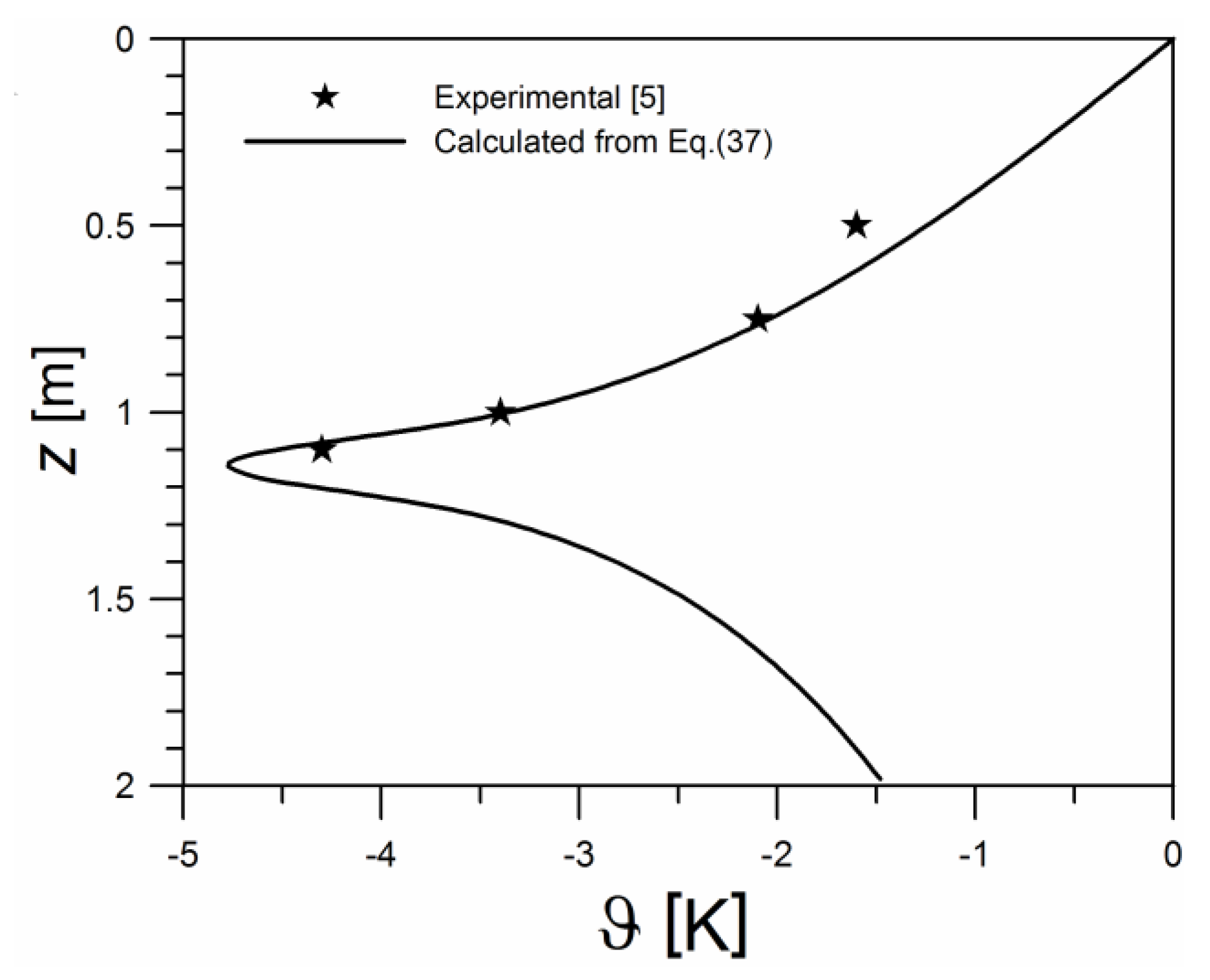
3.6. Comparison with Experimental Results

The computational values of temperature responses are the basis for determining the temperature field for the ground with an installed heat exchanger. The values determined from Equation (37) were compared with the experimental data presented by Wu et al. [5]. The research concerned a slinky-coil exchanger, placed at a depth of 1.14 m, which worked continuously for 52 days with a heat extraction rate equal to 4220 W. The rings were placed in several rows, significantly spaced from each other (4 m).

The calculations of ground temperature responses were conducted for the point corresponding to the location of the temperature measurement sensor (at the wall of one of the rings). The calculations took into account the influence of seven adjacent rings on both sides of the ring under consideration (N_ring = 15).

In order to eliminate the influence of daily changes of ground temperature, only the results of measurements conducted at a depth below 0.5 m were used for comparison. The results of measurements of ground temperature at various levels above the exchanger T and at a large distance from the exchanger T₀ are presented in

Table 3. The results of the experiments presented in [5], and the values ϑ used in Figure 11.

z [m]	T [°C]	T0 [°C]	ϑ = T − T0 [K]
0.50	1.3	2.9	−1.6
0.75	1.8	3.9	−2.1
1.00	1.2	4.6	−3.4
1.14	0.6	4.9	−4.3

.

Figure 11 shows a comparison of the values from Table 3 and those obtained from Equation (37). The compatibility of calculated and experimental values is good.

4. Conclusions

As a result of the theoretical analysis, calculations and simulations of heat transfer in the ground under natural conditions and under conditions with an installed heat exchanger, it was found that:

• Parameters of Equation (2) for determining the undisturbed ground temperature—T_sm, A_s, and P_s—can be calculated from dependencies (23), (28). and (29), derived from the equations of the heat flux balance on the ground surface. Equations of this balance can be solved analytically if the dependencies for the individual heat fluxes are linear with respect to the ground surface temperature T_s. Relation (11) concerning the longwave flux LW and relation (18) concerning the evaporative flux EV satisfy this condition.
• Relationship (18) makes it possible to assess the influence of the solar radiation flux and the annual amount of precipitation on the evaporative flux.
• The time course of heat flux extracted from the ground for space heating with the heat pump q_GHE depends on the maximum heat flux from the ground q_max and the number of heating days in the year h_d. Equations (33)–(35) were proposed to determine this course.
• The ring heat source model was used to find the 3D ground temperature field near a slinky-coil exchanger. In calculations, dependence (37) was used to determine the temperature response caused by the heat sources and Equation (2)—to find the undisturbed ground temperature. The parameters of Equation (2) were specified on the basis of dependencies (23), (28) and (29).
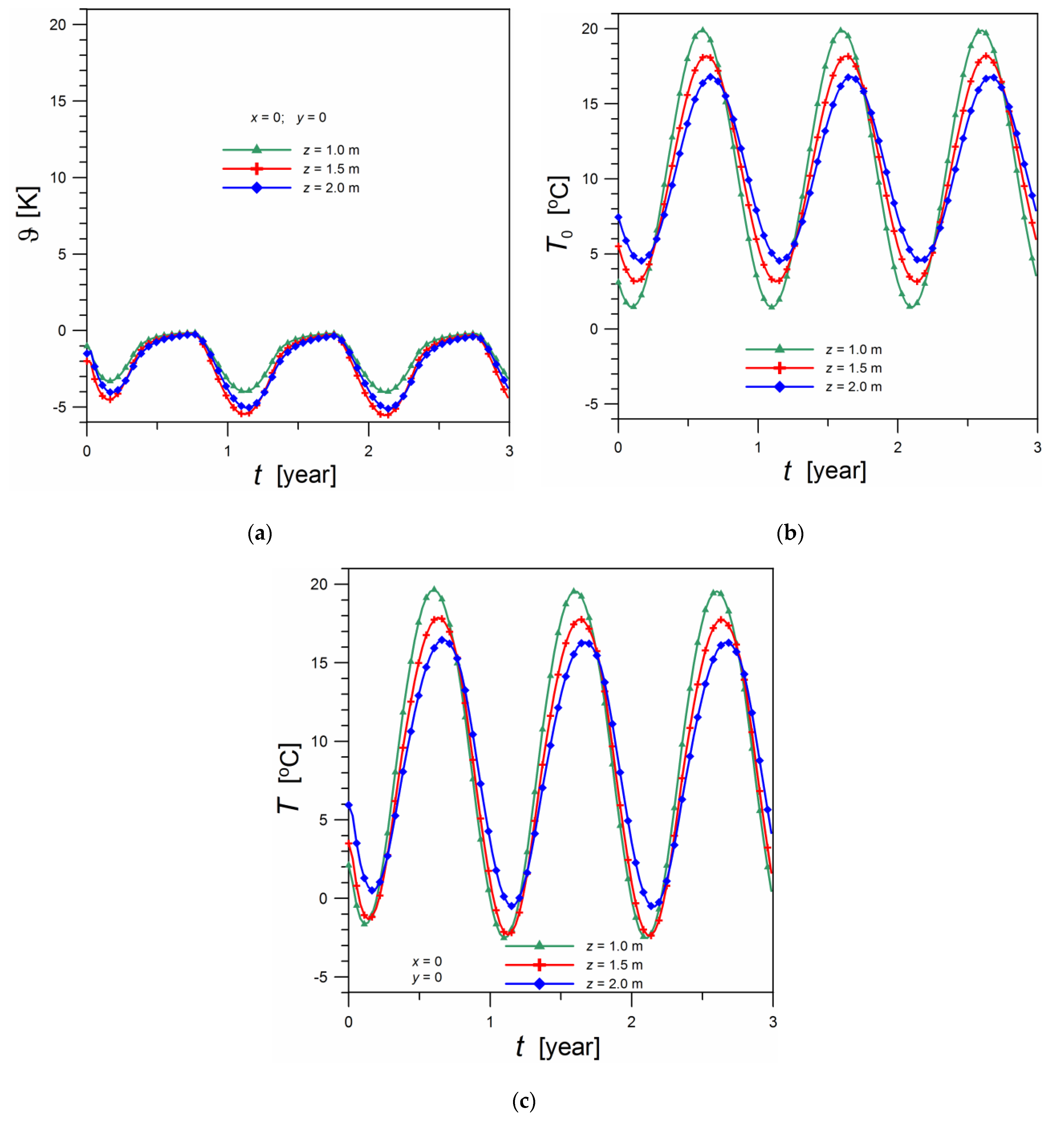
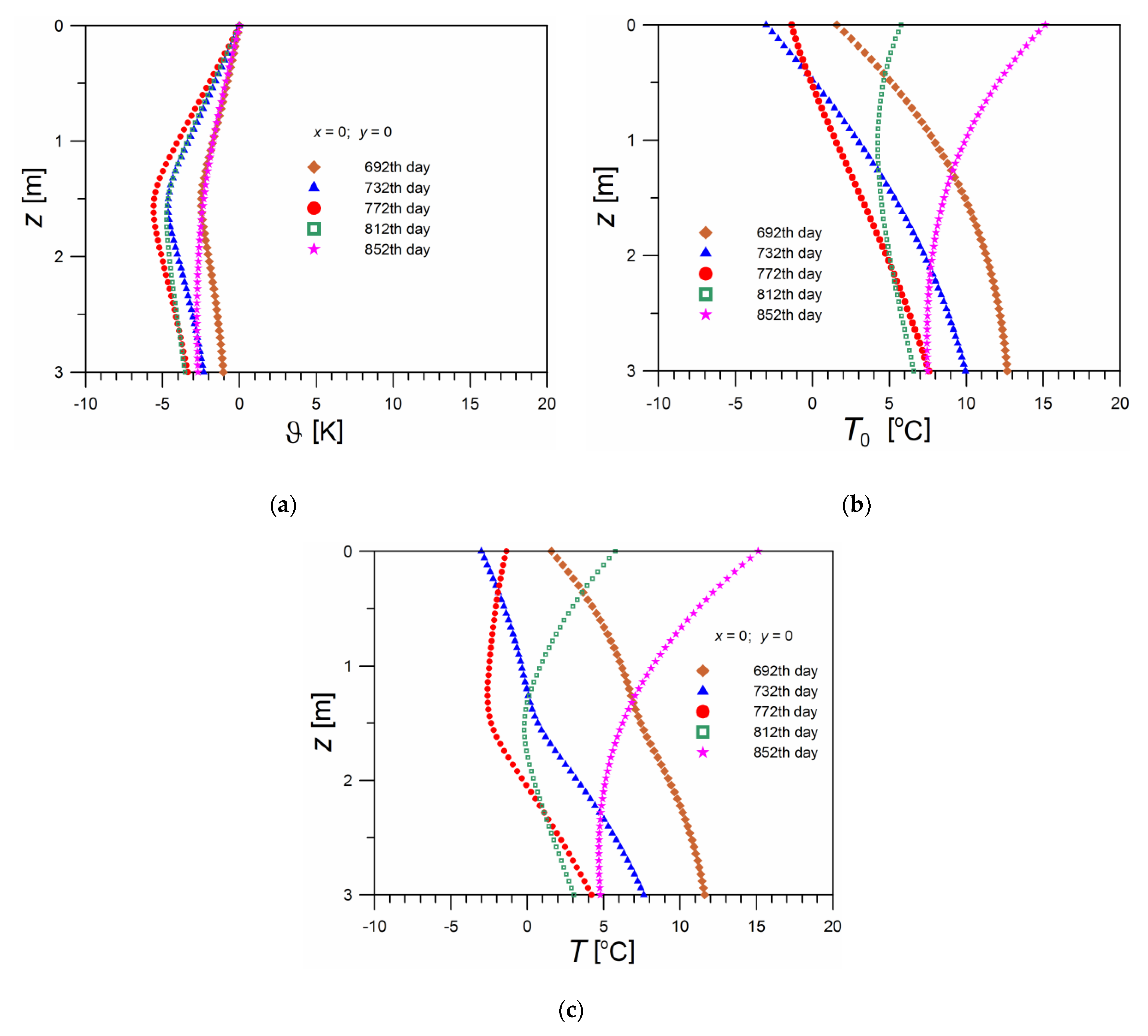
• The influence of spatial variables x and z and time t on the ground temperature was investigated in various combinations. With the use of the superposition principle, it was also shown graphically how the ground temperature is influenced by heat sources and variable ground surface temperature.
• The results of calculations lead to conclusions consistent with those presented in the work by Pauli et al. [6]. Quantitative comparisons were also made by comparing the results of calculations with the results of experiments presented in the study by Wu et al. [5].
• The model used to calculate the temperature field can be used to study the influence of the process parameters on the temperature field near the exchanger pipes. This enables finding such process parameters that prevent the occurrence of dangerously low ground temperature values.

References

1. Shah, T.R.; Ali, H.M. Applications of hybrid nanofluids in solar energy, practical limitations and challenges: A critical review. Sol. Energy 2019, 183, 173–203. [Google Scholar] [CrossRef]
2. Bahiraei, M.; Salmi, H.K.; Safaei, M.R. Effect of employing a new biological nanofluid containing functionalized graphene nanoplatelets on thermal and hydraulic characteristics of a spiral heat exchanger. Energy Convers. Manag. 2019, 180, 72–82. [Google Scholar] [CrossRef]
3. Larwa, B.; Cesari, S.; Bottarelli, M. Study on thermal performance of a PCM enhanced hydronic radiant floor heating system. Energy 2021, 225, 120245. [Google Scholar] [CrossRef]
4. Hepburn, B.D.P.; Sedighi, M.; Thomas, H.R. Field-scale monitoring of a horizontal ground source heat system. Geothermics 2016, 61, 86–103. [Google Scholar] [CrossRef]
5. Wu, Y.; Gan, G.; Verhoef, A.; Vidale, P.L.; Gonzalez, R.G. Experimental measurement and numerical simulation of horizontal-coupled slinky ground source heat exchangers. Appl. Therm. Eng. 2010, 30, 2574–2583. [Google Scholar] [CrossRef] [Green Version]
6. Pauli, P.; Neuberger, P.; Adamovský, R. Monitoring and analysing changes in temperature and energy in the ground with installed horizontal ground heat exchangers. Energies 2016, 9, 555. [Google Scholar] [CrossRef] [Green Version]
7. Neuberger, P.; Adamovský, R. Analysis of the potential of low-temperature heat pump energy sources. Energies 2017, 10, 1922. [Google Scholar] [CrossRef] [Green Version]
8. Neuberger, P.; Adamovský, R. Analysis and comparison of some low-temperature heat sources for heat pumps. Energies 2019, 12, 1853. [Google Scholar] [CrossRef] [Green Version]
9. Jeon, J.-S.; Lee, S.-R.; Kim, M.-J.; Yoon, S. Suggestion of a scale factor to design spiral-coil-type horizontal ground heat exchangers. Energies 2018, 11, 2736. [Google Scholar] [CrossRef] [Green Version]
10. Carslaw, H.S.; Jaeger, J.C. Conduction of Heat in Solids, 2nd ed.; Clarendon Press: Oxford, UK, 1959. [Google Scholar]
11. Kusuda, T.; Achenbach, P.R. Earth temperature and thermal diffusivity at selected stations in the United States. NBS Rep. 1965, 8972, 1–50. [Google Scholar]
12. Allen, R.G.; Pereira, L.S.; Raes, D.; Smith, M. Crop Evapotranspiration-Guidelines for Computing Crop Water Requirements-FAO Irrigation and Drainage Paper 56; Food and Agriculture Organization of the United Nations: Rome, Italy, 1998; Available online: http://www.fao.org/docrep/x0490e/x0490e00.htm (accessed on 29 June 2021).
13. Larwa, B.; Kupiec, K. Study of temperature distribution in the ground. Chem. Process Eng. 2019, 40, 123–137. [Google Scholar] [CrossRef]
14. Incropera, F.P.; Dewitt, D.P.; Bergman, T.L.; Lavine, A.S. Fundamentals of Heat and Mass Transfer, 8th ed.; John Wiley & Sons: Hoboken, NJ, USA, 2017. [Google Scholar]
15. Karn, A.; Chintala, V.; Kumar, S. An investigation into sky temperature estimation, its variation, and signif-icance in heat transfer calculations of solar cookers. Heat Transf. Asian Res. 2019, 4, 1830–1856. [Google Scholar] [CrossRef] [Green Version]
16. Bryś, K.; Bryś, T.; Sayegh, M.A.; Ojrzyńska, H. Subsurface shallow depth soil layers thermal potential for ground heat pumps in Poland. Energy Build. 2018, 165, 64–75. [Google Scholar] [CrossRef]
17. Krakow Klimat (Poland). Available online: https://pl.climate-data.org/europa/polska/lesser-poland-voivodeship/krakow-715022/ (accessed on 4 May 2021).
18. Cengel, Y.A.; Ghajar, A.J. Heat and Mass Transfer: Fundamentals and Applications, 5th ed.; McGrawHill: New York, NY, USA, 2015. [Google Scholar]
19. Howell, T.A.; Evett, S.R. The Penman-monteith Method, Section 3. In Evapotranspiration: Determination of Consumptive Use in Water Rights Proceedings; Continuing Legal Education in Colorado, Inc.: Denver, CO, USA, 2004. [Google Scholar]
20. Tang, F.; Nowamooz, H. Outlet temperatures of a slinky-type horizontal ground heat exchanger with the atmosphere-soil interaction. Renew. Energy 2020, 146, 705–718. [Google Scholar] [CrossRef]
21. Gerrits, A.M.J.; Savenije, H.H.G.; Veling, E.J.M.; Pfister, L. Analytical derivation of the Budyko curve based on rainfall characteristics and a simple evaporation model. Water Resour. Res. 2009, 45, W04403. [Google Scholar] [CrossRef]
22. Budyko, M.I. Climate and Life; Academic Press: New York, NY, USA, 1974. [Google Scholar]
23. Pike, J.G. The estimation of annual runoff from meteorological data in a tropical climate. J. Hydrol. 1964, 2, 116–123. [Google Scholar] [CrossRef]
24. Zhang, L.; Hickel, K.; Dawes, W.R.; Chiew, F.H.S.; Western, A.W.; Briggs, P.R. A rational function approach for estimating mean annual evapotranspiration. Water Resour. Res. 2004, 40, W02502. [Google Scholar] [CrossRef]
25. Krarti, M.; Lopez-Alonzo, C.; Claridge, D.E.; Kreider, J.F. Analytical model to predict annual soil surface temperature variation. J. Sol. Energy Eng. 1995, 117, 91–99. [Google Scholar] [CrossRef]
26. Gwadera, M.; Larwa, B.; Kupiec, K. Undisturbed ground temperature—Different methods of determination. Sustainability 2017, 9, 2055. [Google Scholar] [CrossRef] [Green Version]
27. Badache, M.; Eslami-Nejad, P.; Ouzzane, M.; Aidoun, Z. A new modelling approach for improved ground temperature profile determination. Renew. Energy 2016, 85, 436–444. [Google Scholar] [CrossRef]
28. Khatry, A.K.; Sodha, M.S.; Malik, M.A.S. Periodic variation of ground temperature with depth. Sol. Energy 1978, 20, 425–427. [Google Scholar] [CrossRef]
29. Larwa, B.; Kupiec, K. Heat transfer in the ground with a horizontal heat exchanger installed—Long term thermal effects. Appl. Therm. Eng. 2020, 164, 114539. [Google Scholar] [CrossRef]
30. Xiong, Z.; Fisher, D.E.; Spitler, J.D. Development and validation of a slinky ground heat exchanger model. Appl. Energy 2015, 141, 57–69. [Google Scholar] [CrossRef]
31. Li, H.; Nagano, K.; Lai, Y. A new model and solutions for a spiral heat exchanger and its experimental validation. Int. J. Heat Mass Transf. 2012, 55, 4404–4414. [Google Scholar] [CrossRef]
Figure 1. Linearization of Equation (9).
Energies 14 04010 g001
Figure 2. Linearization of the relationship between the E/P ratio and the aridity index Φ.
Energies 14 04010 g002
Figure 3. Time dependence of the evaporative flux EV for different values of the average solar radiation flux Sm and the annual amount of precipitation P.
Energies 14 04010 g003
Figure 4. Annual temperature courses: air, ground surface, the sky and the gradient of the ground temperature on its surface.
Energies 14 04010 g004
Figure 5. Annual courses of heat flux on the ground surface.
Energies 14 04010 g005
Figure 6. Exemplary time courses of heat flux extracted from the ground.
Energies 14 04010 g006
Figure 7. Arrangement of rings in the simulated system.
Energies 14 04010 g007
Figure 8. Ground temperature profiles along the x axis: (a) temperature response caused by the heat source, (b) undisturbed ground temperature, (c) ground temperature.
Energies 14 04010 g008
Figure 9. Dependence of ground temperature at a given point in time: (a) temperature response caused by the heat source, (b) undisturbed ground temperature, (c) ground temperature.
Energies 14 04010 g009
Figure 10. Ground temperature profiles along the z axis: (a) temperature response caused by the heat source, (b) undisturbed ground temperature, (c) ground temperature.
Energies 14 04010 g010
Figure 11. Comparison of experimental and computational results.
Energies 14 04010 g011