1. Introduction
Gas hydrates (GHs) are solid clathrates consisting of water and hydrocarbon gas (mainly methane). Natural GHs form in permafrost regions or in deep (≥500 m) marine environments offering adequate temperature, pressure, and gas concentration conditions [
1]. Interest in natural GHs has increased in recent decades because of their potential as a future energy source, the possibility of related submarine geohazards, and their impact on global climate change [
2,
3,
4,
5].
Resistivity and P-wave velocity show higher values in the GH-bearing sediments than in the surrounding sediments, which are used to estimate GH saturation from well-log data [
6,
7]. Archie’s equation [
8] can be used to estimate GH saturation from resistivity data [
7], and various rock physics models can be used to estimate GH saturation from velocity data [
9,
10,
11,
12].
The base of the GH stability zone can be predicted from the bottom-simulating reflector (BSR). The seismic method-based determination of the BSR generated by the impedance contrast between sediments with and without GHs is the most reliable way of indirectly confirming GH presence. Some BSRs, such as the opal-A/opal-CT BSR, are not related to GHs but have polarities opposite to those of GH-signifying BSRs [
13].
As indirect seismic data alone may be insufficient for determining GH characteristics in reservoirs, they can be used in combination with well-log data to evaluate GH saturation. Impedance distribution can be obtained by converting seismic data into impedance data using seismic inversion methods. If the relationship between impedance and GH saturation is defined directly or indirectly in well-log data, the GH distribution can be estimated from seismic data. Specifically, the GH distribution can be estimated using the relationship between impedance and porosity [
14,
15] or by directly modeling the density and velocity constituting the impedance changing according to the GH distribution [
16,
17,
18,
19].
Several teams evaluated GH reservoirs in the Ulleung Basin using seismic and well-log data [
20,
21]. Lee et al. [
20] estimated the GH distribution from dense grid 2D seismic and well-log data using seismic inversion and multi-attribute transform techniques. Yi et al. [
21] estimated GH resource volumes from 3D pre-stack seismic data and well-log and core data using pre-stack seismic inversion and rock physics models.
In 2007, the First Ulleung Basin Gas Hydrate Drilling Expedition (UBGH1) obtained well-log data from five sites and cores from three sites, revealing the presence of GHs in mud or thin layers of turbidite sand [
22,
23,
24]. In 2010, the Second Ulleung Basin Gas Hydrate Drilling Expedition (UBGH2) conducted logging while drilling (LWD) and coring at 13 sites to probe the distribution of GH-bearing sediments and find a GH reservoir that could be a potential target for future production tests [
25,
26,
27]. Among the 13 borehole sites explored during UBGH2, UBGH2-6 featured relatively good GH reservoir quality in terms of individual and total cumulative thicknesses of the GH-bearing sand layer [
26].
In deep-sea regions, GH reservoirs can be produced by current technologies as GHs in sand pores. However, most GH-bearing sand layers are thin (several centimeters to several meters thick). Although thin sandy layers filled with GHs can be identified based on high-resolution log data or core data, layers less than 10 m thick are challenging to track using conventional seismic data with a dominant frequency of 30–50 Hz. Although GH distributions obtained using conventional seismic data can help to identify large-scale reservoir units, data availability is limited when detailed information (e.g., in preparation for production testing) is required for each GH-bearing layer.
To overcome the low-resolution problem, the present study proposes a new method of generating high-resolution acoustic impedance volume by performing stepwise seismic inversion using well-log data and two 3D seismic datasets acquired from sources with different frequency ranges. In addition, the high-resolution regional GH distribution is estimated from the acoustic impedance volume based on an established relationship between acoustic impedance and hydrate saturation at site UBGH2-6.
2. Geological Setting
The seafloor spreading that formed the East Sea, a back-arc basin behind the Japanese island (
Figure 1), started in the early Oligocene, stopped in the Middle Miocene because of regional plate reorganization [
28,
29], and was followed by back-closure. As a result, Japan, Yamato, and Ulleung basin separated by raised continental fragments were formed [
30], among which the Ulleung Basin is surrounded by the Korean plateau to the north, the Korean Peninsula to the west, the Oki Bank to the east, and the Japanese islands to the southeast.
Back-arc closure induced deformations (e.g., thrusts, anticlines, folding, and faulting) of the region around the East Sea, including the southern edge of the Ulleung Basin [
31], causing mass flows and continuing until the Pliocene; hence, considerable amounts of sediment were transported to the Ulleung Basin [
32].
Site UBGH2-6 is located in the northwest of the Ulleung Basin and features a water depth of 2153 m. The site was drilled to verify the strong reflectors in seismic section that potentially indicate GH-bearing sand layers overlying mass transport deposits [
25,
26]. At UBGH2-6, core sediments generally consist of hemipelagic muds intercalated with turbidite sands. The thin-to-medium-bedded turbidite sands mainly comprise well-sorted coarse silt to fine sand. The presence of GHs at UBGH2-6 was confirmed at depth of 110–155 mbsf through a combination of infrared core temperature, pore water chlorinity, and pressure core measurements [
26]. GHs in UBGH2-6 usually occur as pore-filling type in many turbidite sands. The GH-bearing sand beds identified in the cores from UBGH2-6 were medium-to-thick bedded, particularly in the deep part of the GH-bearing zone, and well recognized with remarkably high excursions in all resistivity, density, and velocity logs [
26].
3. Data
The study data comprised two 3D seismic datasets obtained from sources with different frequency ranges (
Figure 2) and LWD from the UBGH2-6 well (
Figure 3). Conventional 3D seismic data (C3DS) were acquired for a pretest-production survey around the UBGH2-6 well. Four lines of 324-channel (4000 m long) streamers recorded flip-flop shots from two sets of 1060 in
3 (2000 psi) eight air-gun arrays. The data were recorded at 6.144 s with a sampling interval of 1 ms. The hydrophone group and the shot interval equaled 12.5 and 25 m, respectively. The survey area equaled 250 km
2 (12,000 × 21,000 m), the main direction was northeast-southwest, and the bin size was 25 × 6.25 m. Standard pre-stack time-migration processing was applied to the data. A single-channel sparker seismic survey was conducted to confirm the microscopic displacement of strata around UBGH2-6 and produce high-resolution 3D seismic data (H3DS). The SIG 2-mile sparker system with a 1500 J source (SIG France) was used. The signal was received by a hydrophone streamer with 96 elements (GEO Marine Survey System, Rotterdam, Netherlands). The survey area measured 360 m in the east-west direction and 2200 m in the north-south direction around UBGH2-6. The main survey direction was north-south, and the distance of each line was 20 m. The shot interval was 4 s, which was calculated to be equivalent to ~10 m for a sailing speed of ~5 knots. The sampling and recording times were 0.166 and 4 s, respectively. Each 2D seismic data line was processed using basic techniques, including bandpass filtering, swell effect correction, dephasing, and F-X deconvolution. A 3D grid of 2200 × 360 m and a bin size of 10 × 20 m were designed to properly include all acquired sparker data, and each trace was matched to the 3D grid to create a pseudo 3D volume. The pseudo 3D volume was processed by application of flexible binning, amplitude balancing, post-stack migration, and F-X deconvolution to interpolate missing traces and enhance the signal.
To make the C3DS and H3DS data match, the C3DS grid was rebinned and equated with the H3DS data. The C3DS data were spatially interpolated and rebinned to match the 20 × 10 m bin position and the 0.5 ms sample interval of the H3DS data (
Figure 2).
LWD data included gamma-ray, resistivity, P-wave acoustic, and density logs. The porosity (
Figure 3c) was calculated with bulk density (
ρb), water density (
ρw), and grain density (
ρg). Equation (1) was used to calculate porosity.
From the recovered core analysis results,
ρg and
ρw were determined as 2.64 and 1.02 g/cm
3, respectively. When GHs are present in sediments or clay-rich environments, the neutron porosity is higher than the actual porosity. For this reason, the present study used density porosity, which is known to reflect the porosity of GH-containing sediments more closely [
33,
34]. In addition, Seisspace 4D was used for seismic data matching and Hampson-Russell (version 10) for well-log data analysis and inversion.
4. Workflow and Results
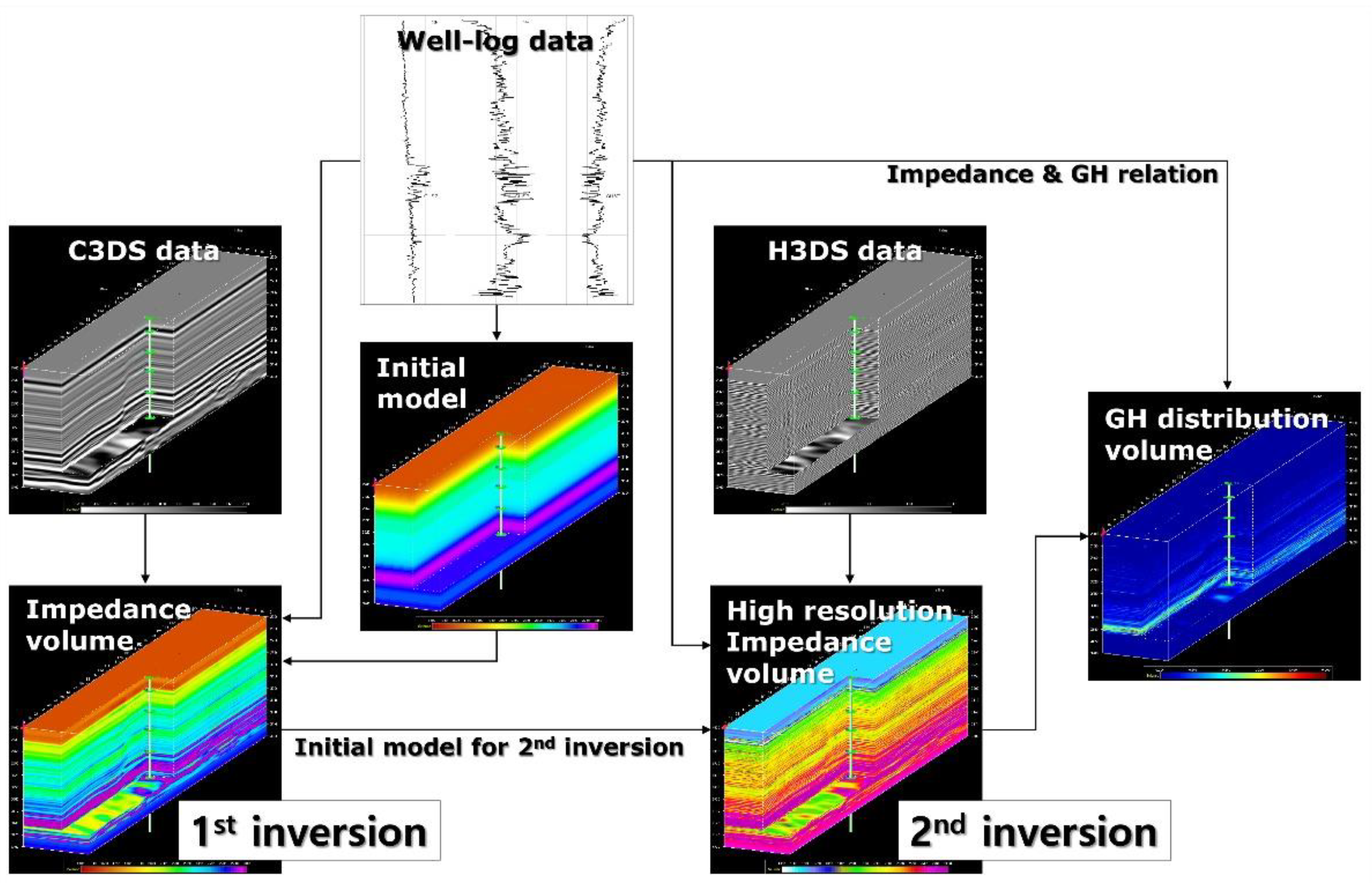
Stepwise seismic inversion was performed using well-log data and two 3D seismic datasets with different effective frequency ranges to produce a high-resolution acoustic impedance volume. The relationship between impedance and GH saturation was defined in the well-log data and used to estimate GH saturation away from the well from inverted high-resolution acoustic impedance data.
Figure 4 shows the data analysis workflow used to obtain high-resolution GH distribution volume.
4.1. Stepwise Seismic Inversion for High-Resolution Impedance Volume
The model-based inversion provided reasonable results even with poor quality of well-log and seismic data. The seismic data give guidelines for inversion, and wavelets can be easily derived from seismic data [
35]. In model-based inversion, an initial impedance model is convolved with the source wavelet to generate a synthetic trace to compare with the seismic trace. The initial impedance model was iteratively altered until the difference between the inverted and seismic traces was reduced to a threshold value. The model with the minimal difference was accepted as a solution. The initial model plays an essential role in providing the low frequencies missing from seismic data to obtain the absolute impedance value and prevent high-frequency details in the model from influencing the final inversion result [
36].
Quantitative prediction of acoustic impedance requires spatially continuous information with a bandwidth of 0 Hz. The missing frequency band below 8 Hz is typically filled in with well-log data because the frequency range of typical marine seismic data starts at ~8 Hz. The initial impedance model was constructed by interpolating the low-frequency components of the impedance logs from the wells. The H3DS data used to estimate the high-resolution absolute impedance volume had a frequency range of 150–600 Hz, which is higher than that of typical marine seismic data used for seismic inversion. To compensate for the missing frequency band below 150 Hz, we used the inversion result of C3DS (typical marine seismic data) as an initial impedance model for the model-based seismic inversion of H3DS data. For the seismic inversion of C3DS data, an initial impedance model for low-frequency below 8 Hz was obtained from the impedance log of the UBGH2-6 well.
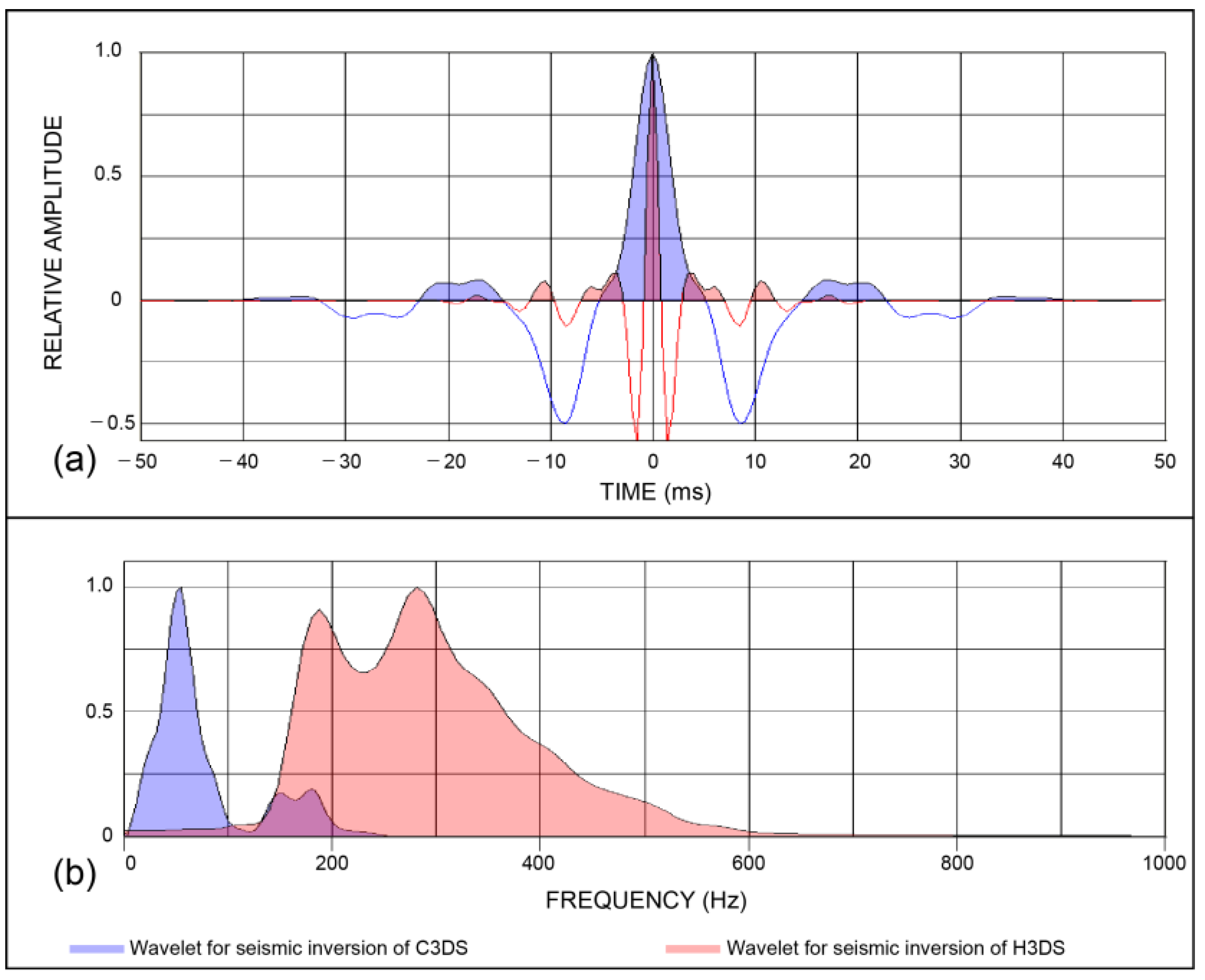
Figure 5 shows the wavelets extracted from each inversion. A wavelet consists of an amplitude and a phase spectrum. We can calculate the amplitude spectrum through autocorrelation of seismic data. However, the phase spectrum cannot be known from seismic data alone, and thus various methods were proposed to predict it [
36]. The seismic data used in the present study were zero-phased through signal processing in the data processing stage, and thus we assumed the phase to be zero and predicted the source wavelet. The wavelet length was set to 100 ms to minimize unnecessary side lobes while maximally reflecting the significant waveform characteristics.
Figure 6 shows the inversion results for C3DS and H3DS at the well location. In each figure, the graph on the left, consisting of three curves, shows the impedance log (blue), the initial model (black), and the inversion result (red). In the middle panel, the two traces comprising 10 identical seismic traces are the synthetic and actual seismic traces at the UBGH2-6, whereas the right panel shows the difference between these two sets of traces. The correlations between the synthetic and actual seismic traces of C3DS and H3DS featured cross-correlation ratios of 0.99948 and 0.999729, respectively. The inversion captured all significant events displayed in the log.
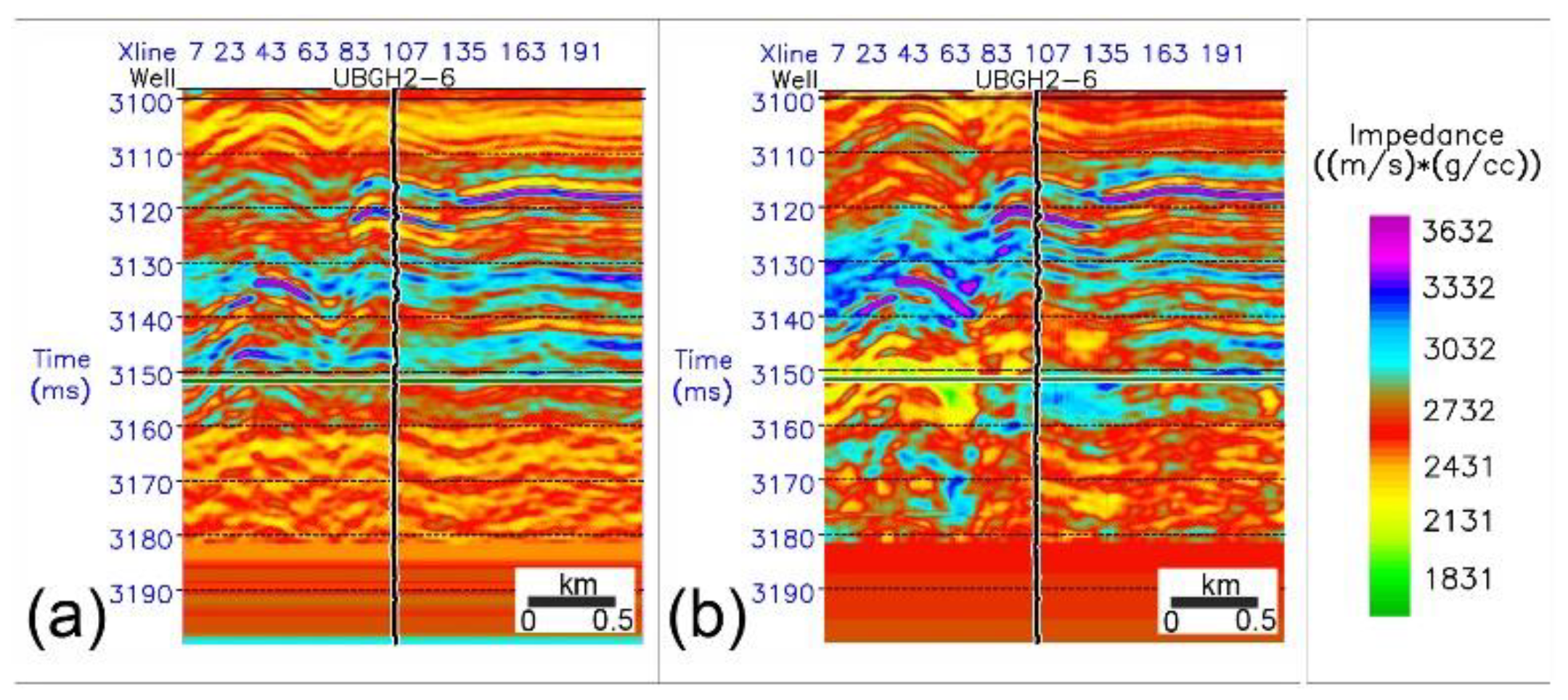
Figure 7e,f show inline 13 and crossline 102 crossing the UBGH2-6 well for the H3DS inversion result. The H3DS inversion result shows that the thin GH-containing sediment layers found at 110–155 mbsf (3100–3150 ms in two-way travel time), which were not recognized by the C3DS inversion, were further subdivided.
4.2. High-Resolution GH Saturation of 3D Seismic Data
Among the physical properties, velocity experiences the most significant changes owing to GH formation in the sediment, increasing with increasing GH content [
37]. The spatial variation in seismic velocity can be used to estimate the spatial variations in GH content [
10]. However, because techniques for inverting the P-wave velocity in seismic data are currently less accessible and less accurate, common seismic inversions produce acoustic impedances that are the product of P-wave velocity and density, especially when post-stack seismic data are used. Lu and McMechan [
14] developed an empirical method for estimating GH saturation from acoustic impedance.
Density porosity is the space filled with fluid, GH, or both [
38]. The water-saturated porosity (
ϕf), or reduced porosity due to the GH, can be expressed as
ϕf = ϕ(1−
Sh), where
ϕ is the total porosity calculated from the density log, and
Sh is GH saturation. When
Sh equals zero, water-saturated porosity is identical to total porosity. When GH replaces all the fluid in the pore, the water-saturated porosity is zero. The GHs in isotropic sediments cause an increase in acoustic impedance and a decrease in water-saturated porosity. In the GH stability zone with pore-filling-type GHs, GH saturation can be estimated using deviations from the baseline, which is the relationship between the porosity of water-saturated sediments and acoustic impedance [
14,
15]. If the total and water-saturated porosities can be predicted in the GH stability zone, GH saturation can be estimated with Equation (2).
where
Sw is water saturation.
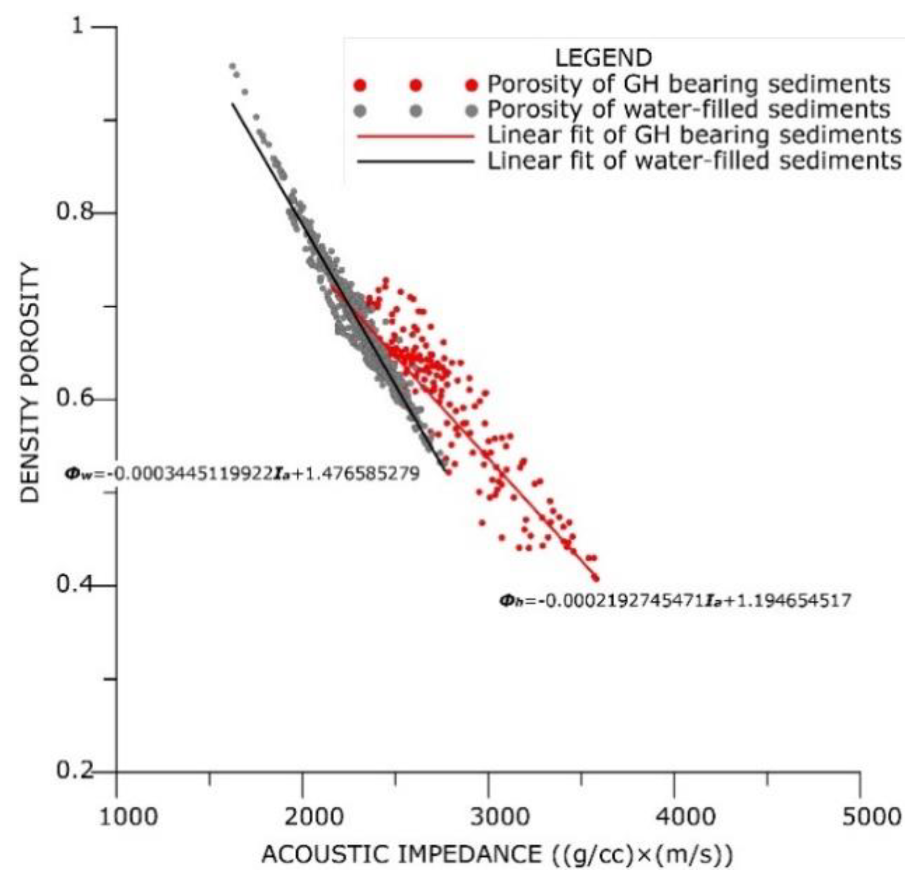
The relationship between acoustic impedance and water-saturated porosity produced an inversely proportional baseline curve when the sediment was homogeneous and compaction was normal in the absence of GHs. In the GH stability zone, GHs in sediments increase acoustic impedance and decrease water-saturated porosity. The deviation from the baseline curve corresponds to GH saturation. The acoustic impedance and porosity (
Figure 8) show a linear relationship for the non-GH-bearing sediments from UBGH2-6 which was given by:
where
is acoustic impedance in (g/cc) × (m/s). The corresponding relationship for the porosity of GH-bearing sediments was fitted as
Assuming that the relationship between water-saturated porosity and acoustic impedance in the GH stability zone follows Equation (3) and that between acoustic impedance and total porosity follows Equation (4), Equation (2) can be rewritten as
Figure 9 shows the GH saturation estimation results at the UBGH2-6 for various methods, in which the saturation estimated from the acoustic impedance log (black) agreed with the saturation estimated from the P-wave velocity log (red) and was generally lower than that calculated from the resistivity log (grey). As the pressure cores were recovered as very small (<1 m long) samples, the corresponding estimates were less representative and showed greater variance.
The information of well-log data can be extended by using seismic data and hence we can gain insights into the study area. Given that the acoustic impedance derived from seismic inversion is the pseudo-acoustic impedance log at each seismic trace, GH saturation can be estimated from seismic data with the method mentioned above. Equation (5) was applied to the respective regions of acoustic impedance volume to obtain GH distribution and saturation (
Figure 10).
5. Discussion
To derive the absolute acoustic impedance using seismic inversion, the method requires the relative acoustic impedance calculated from the input seismic data and the background acoustic impedance to fill in the missing low frequencies [
39,
40]. However, the missing frequency component in the background acoustic impedance model is usually not properly reconstructed, and the estimated acoustic impedance is hence subject to errors owing to the frequency gap. To minimize this error, prior information should be incorporated to close such a gap.
Stepwise seismic inversion was performed to derive a high-resolution acoustic impedance volume with a minimal frequency gap error from high-resolution band-limited H3DS (frequency range 150–600 Hz). The absolute impedance volume calculated from the C3DS data and the well-log data was used as the background acoustic impedance to fill in the low-frequency (~150 Hz) information missing in the H3DS data. We thus obtained the inversion results with an improved resolution that better reflected horizontal heterogeneity than when a seismic inversion was performed using only H3DS (
Figure 11). Despite the above efforts, the seismic data used in this study alone cannot fill the 100–150 Hz gap. Errors from these gaps inevitably result in lower resolution compared to broadband data. The frequency gap can be minimized by strategically designing appropriate seismic sources during the seismic data acquisition stage. If the frequency gap is not large, techniques such as bandwidth extension in the data processing stage may be a solution.
In contrast to explorations that employ the same acquisition specifications for monitoring, such as 4D seismic surveying, the proposed method matched the grid and bin sizes, as two different 3D seismic datasets were used. During the C3DS and H3DS data grid matching for stepwise seismic inversion, we performed spatial interpolation for empty bins where C3DS data traces were not allocated. Although empty bins occurred in ~27% of the grid, the H3DS bin size was sufficiently narrow (20 × 10 m), and the empty bins did not appear continuously (
Figure 12). Therefore, the effect of using C3DS data as an initial model for the seismic inversion of the H3DS data was insignificant.
The inverted acoustic impedance is still different from the acoustic impedance derived from the well-log because of the different seismic and well-log scales. The vertical resolutions of the density log and the P-wave velocity log used to compute the acoustic impedance log were 15.24 and 61 cm, respectively. However, in the GH-bearing zone of the study area, very thin (several decimeters) layers of GH-saturated sands were interbedded in the mud layer in the core [
26]. This resolution limitation resulted in a difference for some areas where the GH-bearing layer was very thin. However, compared to the inversion results of conventional seismic data, the high-resolution acoustic impedance produced by the new method shows that the difference in error values is significantly reduced (
Figure 6).
Uncertainties owing to the difference in scale between GH saturation and impedance in the well comprise the relationship used to convert the acoustic impedance volume to the GH saturation volume. In the UBGH2-6 well-log, the resolution of the impedance (61 cm) was much lower than that of the ring resistivity (5–8 cm). The GH saturations derived from the ring resistivity log and acoustic impedance log showed differences at certain intervals. The GH saturation estimated from pressure core degassing exceeded the values obtained using log-based calculations. The higher GH saturations resulting from degassing resulted from the selective sampling in intervals where GH-bearing signs were evident. The discrepancy between our estimates and the values calculated by other methods most likely resulted from differences in measurement resolutions.
The GH saturation estimation using modifications of previously used methods is subject to the abovementioned uncertainties, which are related to the accuracy of the GH distribution model or the accuracy of the empirical relations and can be decreased through relevant studies. The present study aimed to characterize reservoirs comprising thin GH-bearing layers, which are often found in marine environments. The stepwise seismic inversion method using the two seismic datasets shows that the correlation with well-log data was much better than that obtained when seismic inversion was performed using only conventional seismic data. In addition, the proposed method can be used to identify thin layers much more clearly when acoustic impedance contrast occurs.
6. Conclusions
The GH-distribution estimation suffers from high uncertainty owing to the complexity of GH occurrence and its lateral and vertical heterogeneity. It is not possible to completely overcome the uncertainty associated with scale differences or simplified empirical relationships between data domains (e.g., core, well-log, seismic data). However, if the high-resolution impedance volume can be derived from the data, the uncertainty owing to resolution limitations can be reduced. The present study proposed the stepwise seismic inversion, using two seismic datasets with different frequency bands to characterize a reservoir comprising thin GH layers that frequently appear in marine environments and succeeded in visualizing these thin (tens of centimeters) layers.
The GH distribution around UBGH2-6 was estimated using the high-resolution acoustic impedance volume inverted by the stepwise seismic inversion method and the relationship between water-saturated porosity and acoustic impedance derived from the well-log data.
The low-saturation GH-bearing area was not well constrained owing to the GH saturation error associated with scale differences. However, in the GH reservoir with high GH saturation, the new method was used to characterize the thin GH-bearing layer interbedded in mud layers.
Author Contributions
Conceptualization, B.-Y.Y.; methodology, B.-Y.Y. and Y.-H.Y.; validation, B.-Y.Y. and Y.-H.Y.; formal analysis, B.-Y.Y., Y.-H.Y., G.-Y.K.; investigation (onboard acquisition), B.-Y.Y., Y.-H.Y., Y.-J.K., G.-Y.K., Y.-H.J., N.-K.K., J.-K.K., J.-H.C., and D.-G.Y.; writing—original draft preparation, B.-Y.Y.; writing—review and editing, B.-Y.Y., Y.-H.Y.; project administration, B.-Y.Y. All authors have read and agreed to the published version of the manuscript.
Funding
This study was supported by the Ministry of Trade, Industry and Energy of Korea through the Project “Evaluation of gas hydrate characteristics in the southern part of Korea Plateau (GP2021-009)” under the management of the Gas Hydrate Research and Development Organization of Korea and the Korea Institute of Geoscience and Mineral Resources. This study was also supported by the “Study on Submarine Active Faults and Evaluation of Possibility of Submarine Earthquakes in the Southern Part of the East Sea, Korea (NP2018-018)” of the Ministry of Ocean and Fisheries of Korea.
Institutional Review Board Statement
Not applicable.
Informed Consent Statement
Not applicable.
Data Availability Statement
The data presented in this work are available on request from the corresponding author. The data are not publicly available due to privacy restrictions.
Acknowledgments
The authors would like to thank the captain and crew of the R/V Tamhae II for their efforts and assistance during the seismic survey.
Conflicts of Interest
The authors declare no conflict of interest.
Abbreviations
| GH | Gas hydrate |
| BSR | Bottom-simulating reflector |
| UBGH1 | First Ulleung Basin Gas Hydrate Drilling Expedition |
| UBGH2 | Second Ulleung Basin Gas Hydrate Drilling Expedition |
| LWD | Logging while drilling |
| C3DS | Conventional 3D seismic data |
| H3DS | High-resolution 3D seismic data |
| ρb | Bulk density (g/cm3) |
| ρw | Water density (g/cm3) |
| ρg | Grain density (g/cm3) |
| ϕf | Water-saturated porosity |
| ϕ | Porosity |
| Sh | Gas hydrate saturation |
| Sw | Water saturation |
| Ia | Acoustic impedance (g/cc) × (m/s) |
References
- Kvenvolden, K.A. A Primer in Gas Hydrates. In The Future of Energy Gases: US Geological Survey Professional Paper; Howell, D.G., Ed.; US Geological Survey: Reston, VA, USA, 1993; Volume 1570, pp. 279–292. [Google Scholar]
- Milkov, A.V. Global Estimates of Hydrate-Bound Gas in Marine Sediments: How Much Is Really Out There? Earth Sci. Rev. 2004, 66, 183–197. [Google Scholar] [CrossRef]
- Ruppel, C. Tapping Methane Hydrates for Unconventional Natural Gas. Elements 2007, 3, 193–199. [Google Scholar] [CrossRef]
- Archer, D.E. Methane Hydrate Stability and Anthropogenic Climate Change. Biogeosciences 2007, 4, 521–544. [Google Scholar] [CrossRef] [Green Version]
- Hyndman, R.D.; Yuan, T.; Moran, K. The Concentration of Deep Sea Gas Hydrates from Downhole Electrical Resistivity Logs and Laboratory Data. Earth Planet. Sci. Lett. 1999, 172, 167–177. [Google Scholar] [CrossRef]
- Hovland, M.; Gudmestad, O.T. Potential influence of gas hydrates on seabed installations. In Natural Gas Hydrate: Occurrence, Distribution, and Detection; Paull, C.K., Dillon, W.P., Eds.; American Geophysical Union Geophysical Monograph Series: Washington, DC, USA, 2001; Volume 124, pp. 307–315. [Google Scholar] [CrossRef]
- Collett, T.S.; Ladd, J. Detection of Gas Hydrate with Downhole Logs and Assessment of Gas Hydrate Concentrations (Saturations) and Gas Volumes on the Blake Ridge with Electrical Resistivity Data. Proc. Ocean Drill. Program Sci. Results 2000, 164, 179–191. [Google Scholar]
- Archie, G.E. The Electrical Resistivity Log as an Aid in Determining Some Reservoir Characteristics. Trans. AIME 1942, 146, 54–62. [Google Scholar] [CrossRef]
- Helgerud, M.B.; Dvorkin, J.; Nur, A.; Sakai, A.; Collett, T. Elastic-Wave Velocity in Marine Sediments with Gas Hydrates: Effective Medium Modeling. Geophys. Res. Lett. 1999, 26, 2021–2024. [Google Scholar] [CrossRef]
- Ecker, C.; Dvorkin, J.; Nur, A.M. Estimating the Amount of Gas Hydrate and Free Gas from Marine Seismic Data. Geophysics 2000, 65, 565–573. [Google Scholar] [CrossRef]
- Carcione, J.M.; Tinivella, U. Bottom-Simulating Reflectors: Seismic Velocities and AVO Effects. Geophysics 2000, 65, 54–67. [Google Scholar] [CrossRef]
- Lee, M.W. Models for Gas Hydrate-Bearing Sediments Inferred from Hydraulic Permeability and Elastic Velocities; US Geological Survey Scientific Investigations Report 2008–5219; US Geological Survey: Reston, VA, USA, 2008; p. 20. [Google Scholar]
- Lee, G.H.; Kim, H.J.; Jou, H.T.; Cho, H.M. Opal-A/Opal-CT Phase Boundary Inferred from Bottom-Simulating Reflectors in the Southern South Korea Plateau, East Sea (Sea of Japan). Geophys. Res. Lett. 2003, 30, 2238. [Google Scholar] [CrossRef]
- Lu, S.; McMechan, G.A. Estimation of Gas Hydrate and Free Gas Saturation, Concentration, and Distribution from Seismic Data. Geophysics 2002, 67, 582–593. [Google Scholar] [CrossRef]
- Wang, X.; Wu, S.; Lee, M.; Guo, Y.; Yang, S.; Liang, J. Gas Hydrate Saturation from Acoustic Impedance and Resistivity Logs in the Shenhu Area, South China Sea. Mar. Pet. Geol. 2011, 28, 1625–1633. [Google Scholar] [CrossRef]
- Dai, J.; Snyder, F.; Gillespie, D.; Koesoemadinata, A.; Dutta, N. Exploration for Gas Hydrates in the Deepwater, Northern Gulf of Mexico: Part I. A Seismic Approach Based on Geologic Model, Inversion, and Rock Physics Principles. Mar. Pet. Geol. 2008, 25, 830–844. [Google Scholar] [CrossRef]
- Dai, J.; Banik, N.; Gillespie, D.; Dutta, N. Exploration for Gas Hydrates in the Deepwater, Northern Gulf of Mexico: Part II. Model Validation by Drilling. Mar. Pet. Geol. 2008, 25, 845–859. [Google Scholar] [CrossRef]
- Shelander, D.; Dai, J.; Bunge, G.; Singh, S.; Eissa, M.; Fisher, K. Estimating Saturation of Gas Hydrates Using Conventional 3D Seismic Data, Gulf of Mexico Joint Industry Project Leg II. Mar. Pet. Geol. 2012, 34, 96–110. [Google Scholar] [CrossRef]
- Shankar, U.; Gupta, D.K.; Bhowmick, D.; Sain, K. Gas Hydrate and Free Gas Saturations Using Rock Physics Modelling at Site NGHP-01-05 and 07 in the Krishna-Godavari Basin, Eastern Indian Margin. J. Pet. Sci. Eng. 2013, 106, 62–70. [Google Scholar] [CrossRef]
- Lee, G.H.; Yi, B.Y.; Yoo, D.G.; Ryu, B.J.; Kim, H.J. Estimation of the Gas-Hydrate Resource Volume in a Small Area of the Ulleung Basin, East Sea (Japan Sea) Using Seismic Inversion and Multi-Attribute Transform Techniques. Mar. Pet. Geol. 2013, 47, 291–302. [Google Scholar] [CrossRef]
- Yi, B.Y.; Lee, G.H.; Kang, N.K.; Yoo, D.G.; Lee, J.Y. Deterministic Estimation of Gas-Hydrate Resource Volume in a Small Area of the Ulleung Basin, East Sea (Japan Sea) from Rock Physics Modeling and Pre-Stack Inversion. Mar. Pet. Geol. 2018, 92, 597–608. [Google Scholar] [CrossRef]
- Bahk, J.J.; Um, I.K.; Holland, M. Core Lithologies and Their Constraints on Gas-Hydrate Occurrence in the East Sea, Offshore Korea: Results from the Site UBGH1-9. Mar. Pet. Geol. 2011, 28, 1943–1952. [Google Scholar] [CrossRef]
- Chun, J.H.; Ryu, B.J.; Son, B.K.; Kim, J.H.; Lee, J.Y.; Bahk, J.J.; Kim, H.J.; Woo, K.S.; Nehza, O. Sediment Mounds and Other Sedimentary Features Related to Hydrate Occurrences in a Columnar Seismic Blanking Zone of the Ulleung Basin, East Sea, Korea. Mar. Pet. Geol. 2011, 28, 1787–1800. [Google Scholar] [CrossRef]
- Kim, G.Y.; Yi, B.Y.; Yoo, D.G.; Ryu, B.J.; Riedel, M. Evidence of Gas Hydrate from Downhole Logging Data in the Ulleung Basin, East Sea. Mar. Pet. Geol. 2011, 28, 1979–1985. [Google Scholar] [CrossRef]
- Ryu, B.; Collett, T.S.; Riedel, M.; Kim, G.Y.; Chun, J.; Bahk, J.; Lee, J.Y.; Kim, J.; Yoo, D. Scientific Results of the Second Gas Hydrate Drilling Expedition in the Ulleung Basin (UBGH2). Mar. Pet. Geol. 2013, 47, 1–20. [Google Scholar] [CrossRef]
- Bahk, J.-J.; Kim, G.-Y.; Chun, J.-H.; Kim, J.-H.; Lee, J.Y.; Ryu, B.-J.; Lee, J.-H.; Son, B.-K.; Collett, T.S. Characterization of Gas Hydrate Reservoirs by Integration of Core and Log Data in the Ulleung Basin, East Sea. Mar. Pet. Geol. 2013, 47, 30–42. [Google Scholar] [CrossRef]
- Kim, G.Y.; Narantsetseg, B.; Ryu, B.-J.; Yoo, D.-G.; Lee, J.Y.; Kim, H.S.; Riedel, M. Fracture Orientation and Induced Anisotropy of Gas Hydrate-Bearing Sediments in Seismic Chimney-Like-Structures of the Ulleung Basin, East Sea. Mar. Pet. Geol. 2013, 47, 182–194. [Google Scholar] [CrossRef]
- Sibuet, J.C.; Hsu, S.K.; Le Pichon, X.; Le Formal, J.P.; Reed, D.; Moore, G.; Liu, C.S. East Asia Plate Tectonics Since 15 Ma: Constraints from the Taiwan Region. Tectonophysics 2002, 344, 103–134. [Google Scholar] [CrossRef]
- Lee, G.H.; Yoon, Y.H.; Nam, B.H.; Lim, H.; Kim, Y.-S.; Kim, H.J.; Lee, K. Structural Evolution of the Southwestern Margin of the Ulleung Basin, East Sea (Japan Sea) and Tectonic Implications. Tectonophysics 2011, 502, 293–307. [Google Scholar] [CrossRef]
- Tamaki, K.; Suyehiro, K.; Allan, J.; Ingle, J.C., Jr.; Pisciotto, K.A. Tectonic Synthesis and Implications of Japan Sea ODP Drilling. In Proceedings of the ODP Scientific Results Scientific Results; Part 2; Tamaki, K., Suyehiro, K., Allan, J., McWilliams, M., Eds.; Ocean Drilling Program: College Station, TX, USA, 1992; Volume 127–128, pp. 1333–1348. [Google Scholar]
- Ingle, J.C., Jr. Subsidence of the Japan Sea: Stratigraphic Evidence from ODP Sites and Onshore Sections. In Proceedings Ocean Drilling Program Sci. Results, 127/128; Part 2; Ingle, J.C., Jr., Suyehiro, K., von Breymann, M.T., Eds.; Ocean Drilling Program: College Station, TX, USA, 1992; pp. 1197–1218. [Google Scholar]
- Lee, G.H.; Suk, B. Latest Neogene–Quaternary Seismic Stratigraphy of the Ulleung Basin, East Sea (Sea of Japan). Mar. Geol. 1998, 146, 205–224. [Google Scholar] [CrossRef]
- Riedel, M.; Collett, T.S.; Malone, M.J. The IODP Expedition 311 Scientists. In Proc. IODP, 311; Integrated Ocean Drilling Program Management International, Inc.: Washington, DC, USA, 2006. [Google Scholar] [CrossRef]
- Collett, T.S.; Riedel, M.; Cochran, J.; Boswell, R.; Presley, J.; Kumar, P.; Sathe, A.V.; Sethi, A.; Lall, M.; Sibal, V. The NGHP Expedition 01 Scientists, Geologic Controls on the Occurrence of Gas Hydrates in the Indian Continental Margin: Results of the Indian National Gas Hydrate Program (NGHP) Expedition 01 Initial Reports; U.S. Geological Survey: Reston, VA, USA, 2008; pp. 1–135. [Google Scholar]
- Veeken, P.C.H.; Da Silva, M. Seismic Inversion Methods and Some of Their Constraints. First Break 2004, 22, 47–70. [Google Scholar] [CrossRef]
- STRATA User Guide, Hampson-Russell Assistant: STRATA Theory; Hampson-Russell Software, a CGG Company: Paris, France, 2009.
- Pearson, C.F.; Halleck, P.M.; McGuire, P.L.; Hermes, R.; Mathews, M. Natural Gas Hydrate Deposits: A Review of In Situ Properties. J. Phys. Chem. 1983, 87, 4180–4185. [Google Scholar] [CrossRef] [Green Version]
- Lee, M.W.; Collett, T.S. Elastic Properties of Gas Hydrate-Bearing Sediments. Geophysics 2001, 66, 763–771. [Google Scholar] [CrossRef]
- White, R.; Zabihi Naeini, E. Optimised Spectral Merge of the Background Model in Seismic Inversion. J. Appl. Geophys. 2017, 136, 246–261. [Google Scholar] [CrossRef]
- Guo, S.; Wang, H. Seismic Absolute Acoustic Impedance Inversion with L1 Norm Reflectivity Constraint and Combined First- and Second-Order Total Variation Regularizations. J. Geophys. Eng. 2019, 16, 773–788. [Google Scholar] [CrossRef]
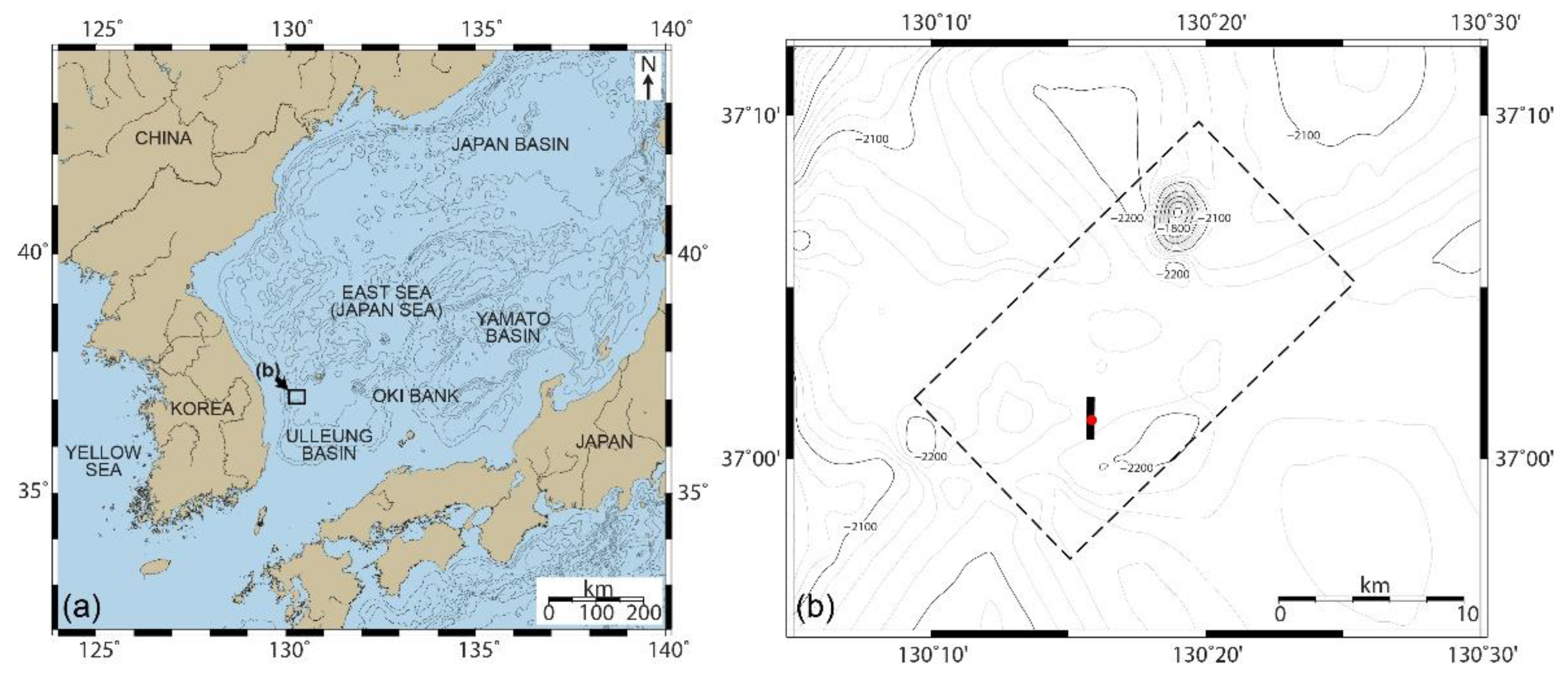
Figure 1.
(
a) East Sea (Japan Sea) physiographic map. The box represents the study area shown in (
b). (
b) Bathymetry of the study area (covering two 3D seismic survey sites) with the UBGH2-6 well location. The dashed and solid boxes indicate the original survey areas of CS3D and HS3D, respectively, shown in
Figure 2. The solid red circle indicates the UBGH2-6 well location. Contours are in meters.
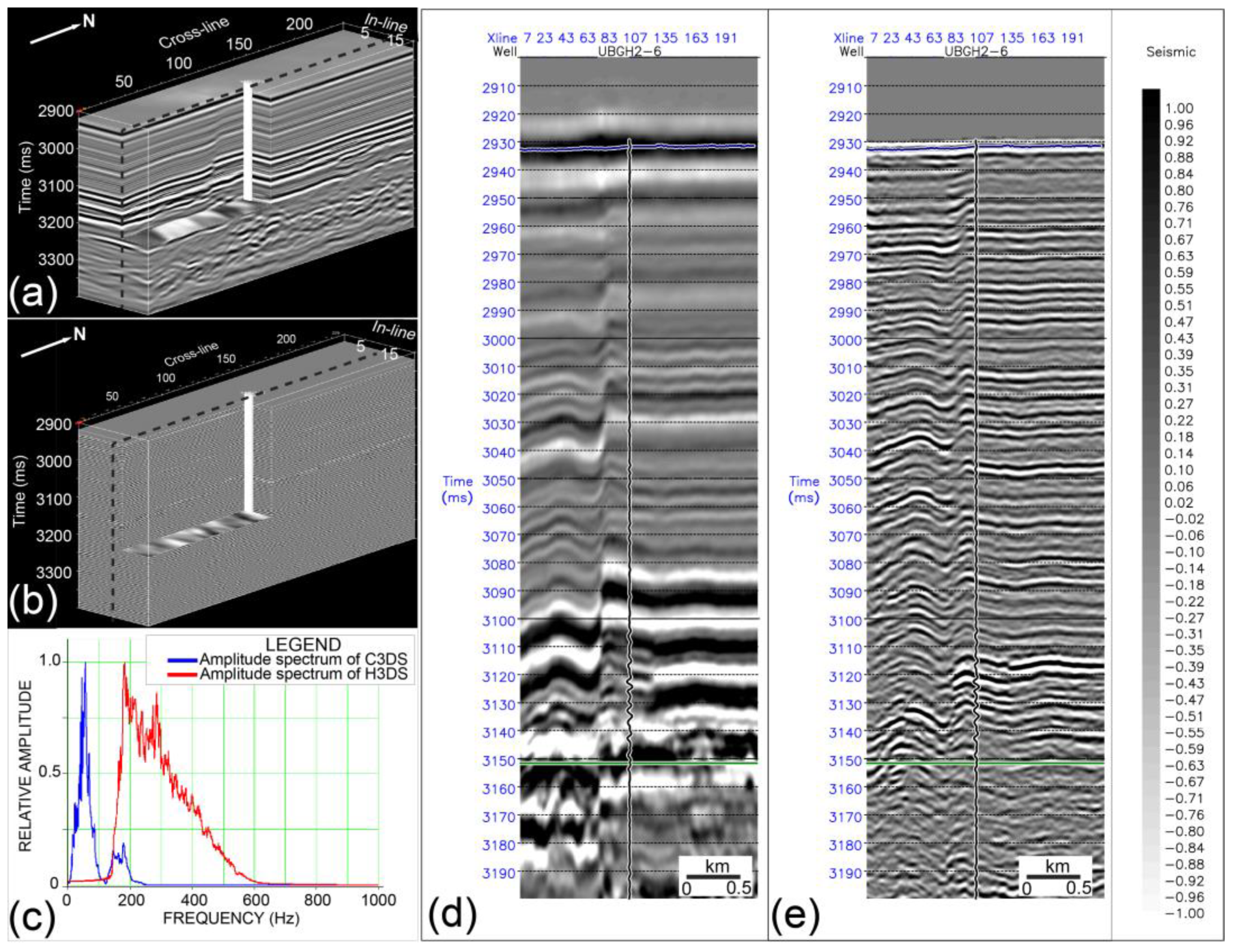
Figure 2.
Two different 3D seismic datasets used in this study consist of 19 inlines (20 m interval) by 240 crosslines (10 m interval). (a,b) show rebinned CS3D and HS3D volume, respectively. (c) CS3D and HS3D amplitude spectra. (d,e) show seismic inline 13 of CS3D and HS3D crossing the UBGH2-6 well, respectively.
Figure 3.
(a) P-wave velocity, (b) bulk density, and (c) density porosity in the UBGH2-6 well. Density porosity was computed from bulk density with the average matrix density (2.64 g/cm3) and fluid density (1.02 g/cm3).
Figure 3.
(a) P-wave velocity, (b) bulk density, and (c) density porosity in the UBGH2-6 well. Density porosity was computed from bulk density with the average matrix density (2.64 g/cm3) and fluid density (1.02 g/cm3).
Figure 4.
Data analysis workflow. The GH distribution volume was estimated from two seismic inversions with two different 3D seismic datasets and UBGH2-6 well-log.
Figure 4.
Data analysis workflow. The GH distribution volume was estimated from two seismic inversions with two different 3D seismic datasets and UBGH2-6 well-log.
Figure 5.
(a) Two wavelets extracted from C3DS and H3DS. (b) Amplitude spectra for the two wavelets shown in (a).
Figure 5.
(a) Two wavelets extracted from C3DS and H3DS. (b) Amplitude spectra for the two wavelets shown in (a).
Figure 6.
(a) C3DS and (b) H3DS seismic inversion results at the UBGH2-6 well. The left panel in each figure shows three curves: initial model impedance (black), original log (blue), inversion result (red). The middle panel in each figure shows synthetic (red) and actual seismic (black) traces. The right panel in each figure shows the error traces (difference between synthetic and real seismic traces). The inversion results match well with the derived impedance from the well-log. The cross-correlation ratio between synthetic and seismic traces is 0.99948 for (a) and 0.999729 for (b).
Figure 7.
Inline 13 and crossline 102 crossing the UBGH2-6 well. (a,b) Initial model for the C3DS seismic inversion, and inversion result for (c,d) C3DS and (e,f) H3DS. Black lines inserted in each figure show the acoustic impedance log of the UBGH2-6 well.
Figure 7.
Inline 13 and crossline 102 crossing the UBGH2-6 well. (a,b) Initial model for the C3DS seismic inversion, and inversion result for (c,d) C3DS and (e,f) H3DS. Black lines inserted in each figure show the acoustic impedance log of the UBGH2-6 well.
Figure 8.
Plot of density porosity vs. acoustic impedance at the UBGH2-6 well. Red and grey dots indicate the porosity of GH-bearing and non-GH-bearing sediments, respectively.
Figure 8.
Plot of density porosity vs. acoustic impedance at the UBGH2-6 well. Red and grey dots indicate the porosity of GH-bearing and non-GH-bearing sediments, respectively.
Figure 9.
GH saturation estimated with various methods at the UBGH2-6 well. The black line shows the GH saturation estimated using Equation (5) in this study. Grey line indicates the GH saturation estimated from the resistivity log. Red line refers to the GH saturation estimated from the P-wave velocity. Black dots show the GH saturation estimated from pressure core degassing.
Figure 10.
GH saturation estimated with Equation (5) for (a) inline 13 and (b) crossline 102 of C3DS and (c) inline 13 and (d) crossline 102 of H3DS crossing the UBGH2-6 well.
Figure 10.
GH saturation estimated with Equation (5) for (a) inline 13 and (b) crossline 102 of C3DS and (c) inline 13 and (d) crossline 102 of H3DS crossing the UBGH2-6 well.
Figure 11.
(a) Result of inversion with well-log and H3DS data only. Because the initial model to reduce uncertainty from missing low-frequency in H3DS data is composed of well-log only, the impedance shows periodical anomalies without reflecting lateral changes in the strata. (b) Result of stepwise seismic inversion using the inversion result of C3DS as a low-frequency initial model. Results reflect well the lateral changes of the strata.
Figure 12.
C3DS bin fold map after matching to the H3DS data. Blue dots show the location of empty bins, which are interpolated via surrounding traces.
Figure 12.
C3DS bin fold map after matching to the H3DS data. Blue dots show the location of empty bins, which are interpolated via surrounding traces.
| Publisher’s Note: MDPI stays neutral with regard to jurisdictional claims in published maps and institutional affiliations. |
© 2021 by the authors. Licensee MDPI, Basel, Switzerland. This article is an open access article distributed under the terms and conditions of the Creative Commons Attribution (CC BY) license (https://creativecommons.org/licenses/by/4.0/).


 ,
, 