An Estimation of the Lightweight Potential of Battery Electric Vehicles

Abstract

Although battery electric vehicles (BEVs) are locally emission-free and assist automakers in reducing their carbon footprint, two major disadvantages are their shorter range and higher production costs compared to combustion engines. These drawbacks are primarily due to the battery, which is generally the heaviest and most expensive component of a BEV. Lightweight measures (strategies to decrease vehicle mass, e.g., by changing materials or downsizing components) lower energy consumption and reduce the amount of battery energy required (and in turn battery costs). Careful selection of lightweight measures can result in their costs being balanced out by a commensurate reduction in battery costs. This leads to a higher efficiency vehicle, but without affecting its production and development costs. In this paper, we estimate the lightweight potential of BEVs, i.e., the cost limit below which a lightweight measure is fully compensated by the cost savings it generates. We implement a parametric energy consumption and mass model and apply it to a set of BEVs. Subsequently, we apply the model to quantify the lightweight potential range (in €/kg) of BEVs. The findings of this paper can be used as a reference for the development of cheaper, lighter, and more energy-efficient BEVs.

1. Introduction

Over the past decade, the emission limits set by the European Union for new passenger cars have become increasingly stringent [1]. One effective way for vehicle manufacturers to lower their fleet emissions and comply with the European regulations is to produce battery electric vehicles (BEVs) [2]. However, a major obstacle for BEVs remains their lower range compared to internal combustion engine vehicles (ICEVs) [3]. For this reason, range is a crucial selling point for BEVs [4,5]. One strategy that can guarantee a certain target range is to reduce the vehicle’s consumption, which depends on external and internal resistances.

External resistances are associated with rolling, aerodynamics, climbing, and acceleration resistance ([6] p. 137) [7]. The former is caused by deformation of the tire during vehicle motion [7] and can be described with the tire rolling coefficient f_RR, the mass of the vehicle m_veh, the gravitational acceleration g, and the road inclination angle α:

F_Rolling = m_veh × g × f_RR × cos(α)

(1)

The aerodynamic resistance F_Aerodynamic is caused by air friction and pressure differences between the front and the rear of the vehicle [8] (p. 14). It depends on the vehicle’s frontal area A_f, its drag coefficient c_d, its speed v_veh, and the air density ρ_air:

F_Aerodynamic = c_d × A_f × ρ_air × v_veh²/2

(2)

The acceleration resistance F_Acceleration is caused by the inertia of the vehicle and its rotating parts. This resistance is modeled based on the acceleration of the vehicle a_veh, its mass, and the rotational mass factor e_i [9] (p. 10):

F_Acceleration = m_veh × e_i × a_veh

(3)

Finally, the slope resistance F_Slope is induced by gravity when the vehicle drives on a non-horizontal road. It depends on vehicle mass, gravitational acceleration, and road inclination angle α [8] (p. 16).

F_Slope = m_veh × g × sin(α)

(4)

The total external resistance is obtained by adding up rolling, drag, acceleration, and slope resistance. As shown in Equations (1)–(4), three out of four components of the external resistance are mass-dependent. In order for the vehicle to follow a defined speed profile, it has to overcome these.

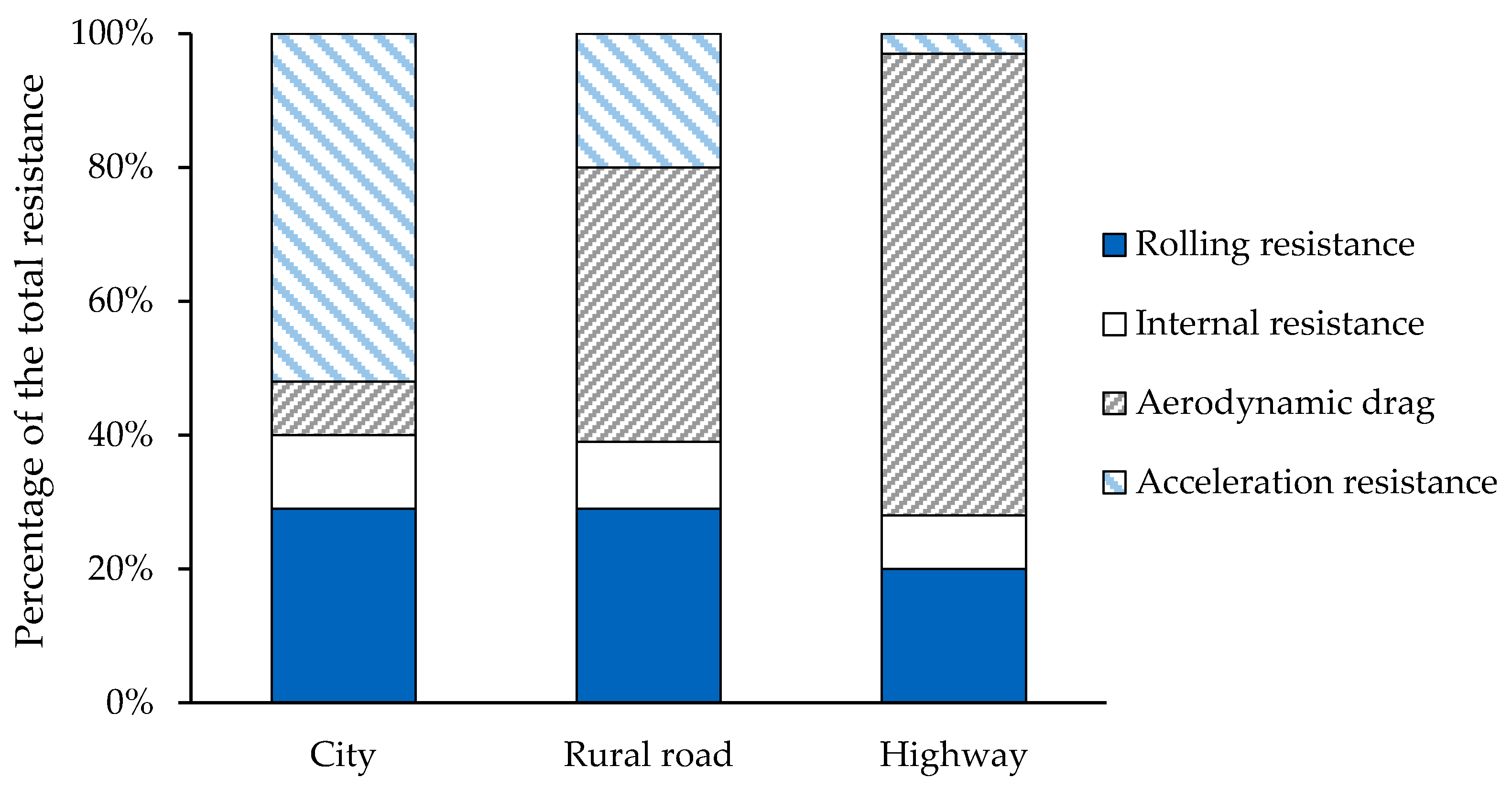
Internal resistances describe losses within components caused by friction as well as the energies required for auxiliary units [10] (p. 34). An example are gearbox losses, which are composed by gear, bearing, and load independent losses.

Figure 1 outlines the percentage contributions of internal and external resistances (the slope resistance is excluded) in three different scenarios: city, rural road, and highway. Mass-dependent resistances account for approximately 92% of the losses in the city scenario, 55% in the rural road scenario, and 30% in the highway scenario [10] (p. 35).

Figure 1 and Equations (1)–(4) show the strong correlation between mass and energy consumption. Reducing vehicle mass is consequently an effective strategy for decreasing energy consumption and achieving the target range. Furthermore, the lower the vehicle’s consumption, the less battery energy is needed to attain the target range. This is significant for two reasons. First, a lower energy demand means lower battery costs. Since the role of the battery is a key element of the vehicle cost structure [11], reducing its cost will have a significant impact on the total vehicle costs. Second, as the gravimetric energy density of lithium-ion batteries is lower than that of gasoline and diesel fuels [12], a decrease of a few kWh can result in a considerable mass reduction [13], leading to a further drop in energy consumption.

The high cost of lithium-ion batteries combined with their low gravimetric energy density make mass reduction strategies (lightweight measures) particularly attractive for BEVs. However, every lightweight measure also generates costs [14] (p. 49). For example, vehicle mass can be reduced by investing in lighter (but also more expensive) materials for the body in white (BIW). Such a strategy is being pursued with the BMW i3, whose body is largely made of carbon fibers [15].

Lightweight measures are therefore an important strategic choice during the early development of BEVs. In the best-case scenario, the investment required for a lightweight measure can be partially or even fully compensated by the reduction in battery energy (and thus the costs) it generates. To create such a scenario, we must define the circumstances under which a lightweight measure can compensate its costs, by answering the question: What is the lightweight potential of BEVs? The purpose of the present paper is to answer this question. However, before we can investigate the lightweight potential of BEVs, we first have to understand the influence that a lightweight measure has on the vehicle.

The paper is structured as follows: after explaining the importance of lightweight measures (Section 1.1) the state of the art is evaluated (Section 1.2) and the research gap identified (Section 1.3). Based on the research gap, a tool to quantify the mass and lightweight potential of BEVs is presented (Section 2). Section 3 provides a validation of the presented tool using a dataset of existing BEVs. The approach is then applied in Section 4 to quantify the lightweight potential of current BEVs. Section 5 and Section 6 close the paper with a discussion and outlook.

1.1. Primary and Secondary Mass Reduction in the Early Development Phase

To understand the impact of a lightweight measure on a vehicle, we first have to briefly explain the BEV development process. During the early development phase of a BEV, concept engineers compile a detailed portfolio of requirements for the vehicle. This includes design parameters such as acceleration time, maximum speed, and target range [16]. In subsequent development steps, the vehicle components are detailed and sized according to the portfolio target values. This results in an initial dimensioning of the vehicle’s components and an estimation of its mass and costs.

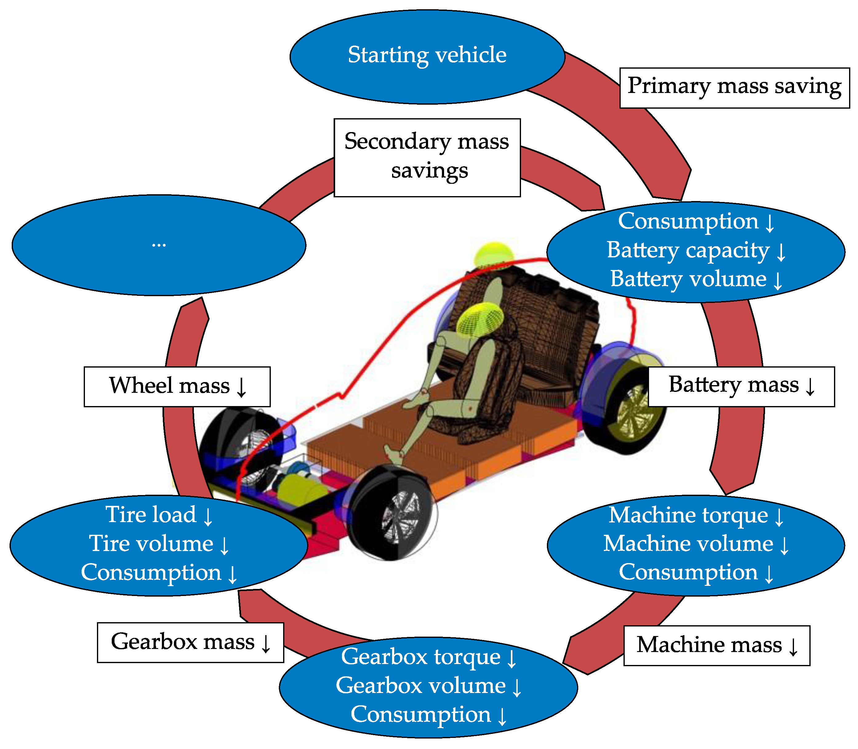
What will happen if a lightweight measure is applied at this stage of development? The lightweight measure will cause a reduction in vehicle mass, which we will define as a primary mass saving (PMS). This will cause consumption to decrease, setting a mass spiral in motion (Figure 2).

Due to the resulting lower energy consumption, a smaller battery pack will now be sufficient to create the target range required in the vehicle portfolio. Electric machines and gearboxes can then also be downsized, as less torque is required to fulfill the required acceleration time and maximum speed. These adjustments are propagated to other mass-dependent components, such as the wheels, suspension system, and BIW. The mass savings induced by the spiral are referred to as secondary mass savings (SMSs). These SMSs can themselves trigger further SMSs (Figure 2).

One way of quantifying the SMSs is with the secondary to primary ratio (SPR), which expresses the relationship between the SMSs and the PMS which induces them [17] (pp. 9–10) according to Equation (5). For example, an SPR of 0.5 means that given a mass reduction of 100 kg, a secondary mass saving of 50 kg is possible.

SPR = SMS/PMS

(5)

For vehicles equipped with an electric powertrain, the SMSs induced by a lightweight measure further reduce the battery energy required, thus decreasing the vehicle’s production and development costs. In the case of ICEVs, this reduction is in the required tank capacity, which, however, has little impact on vehicle costs.

Figure 2. A mass spiral showing the SMSs generated from a lightweight measure. Based on [18].

Figure 2. A mass spiral showing the SMSs generated from a lightweight measure. Based on [18].

Therefore, to quantify the lightweight potential of BEVs, it is necessary to model the component masses (for assessing SPR and SMSs) and the correlation between mass and energy consumption (to estimate the savings in battery energy). The following section reviews the work of some authors who have attempted to address this problem.

1.2. Existing Methods of Modeling Lightweight Potential

In the early development phase, several researchers were concerned with the key role of mass reduction. To address the problem, parametric models were developed to simplify the problem of mass estimation (

Table 1. Overview of existing methods of vehicle mass estimation. Based on [13].

Author	Year	BEV Considered?	Modeling of SMSs
Malen et al. [19]	2007	No	Yes
Gobbels et al. [20]	2010	No	Yes, with finite element simulations
Yanni et al. [21]	2010	No	No
Alonso et al. [22]	2012	No	Yes
Fuchs [17,23]	2014	Yes	Yes
Wiedemann [24]	2014	Yes	Yes, on powertrain components
Mau et al. [25]	2016	No	No
Felgenhauer et al. [26]	2019	Yes	No

).

Malen et al. [19] divided the vehicle into 13 subsystems and assigned a secondary mass coefficient to each subsystem. These coefficients describe the incremental mass change in the corresponding subsystem for a unit change in gross vehicle mass and are determined by empirical analysis of a dataset of 32 ICEVs. The sum of the subsystem’s secondary mass coefficients yields the SPR. According to the authors, fuel and exhaust systems as well as electrical, cooling, and closure systems have low coefficients and hence experience little mass fluctuation. Malen et al. [19] estimate an SPR of between 0.8 and 1.5 if all subsystems are resized. When the powertrain is not available for resizing, the SPR drops to a range between 0.4 and 0.5.

Gobbels et al. [20] propose a method of quantifying SMSs in passenger cars. The vehicle components are modeled separately and organized into six subsystems (body, engine, transmission, suspensions, interior, and electronics). For the body and suspensions, the mass reduction potential is determined by finite element simulations. The engine and transmission subsystems are described by regression models, while the interior and electronics subsystems are regarded as mass-independent. The modeling is based on two reference vehicles, an Opel Corsa C and a Volkswagen Golf VI. The approach predicts an SPR of 0.30 for the Opel Corsa and 0.46 for the Volkswagen Golf.

Yanni et al. [21] derive a linear regression model to estimate the vehicle mass based on its power and external dimensions. However, the authors did not consider BEVs, and the resulting estimation only includes SMSs that result from a change in the vehicle’s external dimensions.

Alonso et al. [22] follow the same approach defined by Malen et al. [19] and develop an empirical method to determine how the different subsystems are affected by a change in the overall vehicle mass. The modeling follows an empirical approach, based on a dataset of 77 ICEVs. The authors do not consider BEVs, though, and focus exclusively on combustion engines, estimating an SPR of 0.49.

Fuchs et al. [17,23] divide the vehicle into eight subsystems to create a parametric mass model. Each subsystem is further divided into subcomponents, which are modeled with empirical and semi-physical models. A dataset of 24 vehicles (including BEVs and ICEVs) is used to derive the empirical models. The authors couple the parametric mass model with an energy consumption simulation, which is used to size the powertrain and quantify the vehicle consumption. The research done by Fuchs et al. [17] highlights the large impact of target range and battery energy on the mass of BEVs. In a simulation of a two-seater BEV with a range of 150 km, the authors predict an SPR of between 0.32 and 0.45.

Wiedemann [24] develops a parametric model for BEVs which also includes a parametric mass calculation. He estimates a basic vehicle mass using the model of Yanni et al. [21]. The mass of the electric powertrain is modeled by adding the contributions of battery, electric machine, power electronics, and gearbox, which are all estimated using empirical models. As with Fuchs, Wiedemann also implements an energy consumption simulation to model the interdependencies between vehicle mass and consumption. Wiedemann’s model can estimate the SMSs, but only on the powertrain components.

Mau et al. [25] divide the vehicle into seven subsystems, and model each subsystem empirically. For example, powertrain mass is calculated based on engine torque, gearbox type, and drive configuration (front/rear/all-wheel drive). However, the model does not consider BEVs or SMSs.

Finally, Felgenhauer et al. [26] develop an empirical regression model based on the methods of Mau and Yanni [21,25]. The model includes BEVs but can only estimate SMSs resulting from a change in the vehicle’s external dimensions.

1.3. Research Gap

Among the authors listed in Table 1, only Malen et al. [19], Gobbels et al. [20], Fuchs [17], and Alonso et al. [22] consider all mass-dependent vehicle subsystems when modeling the SMSs. Fuchs is the only author to include BEVs in an energy consumption simulation.

Apart from the fact that the empirical data employed by Fuchs is outdated (the database he uses includes vehicles built before 2013), another disadvantage (which is true of all approaches in Table 1) is that the author does not model the vehicle package but focuses on its mass. Transferred to a practical example, Fuchs’ parametric model is able to quantify the number of kWh the battery is required to store to reach a certain range but it cannot estimate whether the simulated vehicle can accommodate this energy. This is particularly critical since the lightweight potential derived might be calculated on the basis of vehicles that are not feasible in the first place.

To address these issues, the parametric mass model presented in this paper estimates the mass of BEVs using an approach similar to that of Fuchs [17] but employing an up-to-date vehicle dataset. Moreover, the model is encapsulated by a vehicle architecture tool that includes an energy consumption simulation and a package model. The former calculates the energy consumption and estimates the battery energy requirements depending on the vehicle mass and target range. The latter sizes and positions the components and checks the feasibility of the vehicle. This ensures that the simulated vehicle is feasible in terms of energy consumption, mass, and package. All the parts of the vehicle architecture tool (energy consumption, parametric mass model, and package model) are implemented in MATLAB.

2. Materials and Methods

The first part of this section briefly discusses the workflow of the vehicle architecture tool. This is followed by detailing of the parametric mass model.

2.1. Vehicle Architecture Tool

The inputs of the tool correspond to the content of the portfolio defined by the concept engineers (Section 1.1) and include variables such as acceleration time, vehicle speed, electric range, and initial vehicle mass m₀ (Step 1, Figure 3). The tool inputs are listed in

Table A1. Required Inputs for the vehicle architecture tool.

Required Inputs
Parameter	Unit
Acceleration time from 0 to 100 km/h	s
Air suspension	Yes/No
All-wheel steering	Yes/No
Aluminum percentage in the frame	%
Body style (sedan, hatchback, SUV)	–
Cell type (prismatic, pouch, cylindrical)	–
Cluster type	Digital/Analog
Door material	Steel/Aluminum
Driver seating height (H30-1)	mm
Driving cycle for vehicle consumption (WLTP, NEDC, etc.)	–
Electric Machine number and type (IM, PMSM)	–
Electric range	km
Fenders material	Steel/Aluminum
Gearbox transmission ratio	–
Gearbox type (coaxial, parallel axles)	–
Gravimetric energy density at the cell level	Wh/kg
Hatch material	Steel/Aluminum
Head up Display	Yes/No
Headlights type	LED/Xenon/Halogen
Hood material	Steel/Aluminum
Maximum speed	m/s
Number of doors	2/4
Number of seats	–
Overhang front and rear (L104, L105)	mm
Panorama roof	Yes/No
Sliding rear seats	Yes/No
Sliding roof	Yes/No
Subwoofer	Yes/No
Tire diameter	mm
Tire type (Extra load, Normal load)	-
Vehicle height (H100)	mm
Vehicle wheelbase (L101)	mm
Vehicle width (W103)	mm
Volumetric energy density at the cell level	Wh/l

.

Based on these inputs, the requirements of the electric powertrain (such as electric machine power and required battery energy) are derived with an energy consumption simulation (Step 2, Figure 3). The consumption simulation is available as an open-source MATLAB code in [27] and documented in [7].

In the third step, the vehicle components are sized and positioned by a package model. Here, the components are modeled using empirical and semi-physical models. The outcome of this step is a rough layout of the vehicle package. Several components of the package model have been discussed in previous publications [5,13,28].

Following the package modeling, the component masses are estimated with the parametric mass model (Step 4, Figure 3). The vehicle components are organized into seven modules and the mass of each module derived empirically. For the modeling, the inputs given in Step 1 are combined with the results of the energy consumption simulation and the package model. The total mass of the vehicle is derived by totaling the contributions of the seven modules. This step yields the new mass estimate m₁.

At this point, m₁ is compared with the mass m₀ assumed in Step 1. If the difference between the two values is above a certain tolerance, a new iteration is required. Then, m₁ is reintroduced in the LDS and the new power and energy requirements calculated. Due to the changed requirements, the components are also sized differently, which impacts the vehicle package. The iterative process continues until the difference between the masses of two consecutive iterations n and n − 1 falls below a given tolerance $\epsilon$ (which is set to a default value of 5 kg). For each iteration, the tool not only tests the feasibility of the target range and power as a function of the mass but also ensures that the vehicle package is feasible.

If the mass does not converge after ten consecutive iterations, the tolerance $\epsilon$ is stepwise increased. Otherwise the approach outputs the resulting vehicle package. Figure 4 shows a typical output of Step 5.

Figure 3. Overview of the vehicle architecture tool based on [5,29]. The tool is implemented entirely in MATLAB.

Figure 3. Overview of the vehicle architecture tool based on [5,29]. The tool is implemented entirely in MATLAB.

2.2. Parametric Mass Model

To implement the parametric mass model, we define seven modules: frame, chassis, powertrain, exterior, interior, electrics, and accessories. The modules are divided into subsystems, which are modeled separately using empirical models such as linear regression and constant values (the latter based on normal distributions). The empirical models are derived using the method documented in [30]. In total, more than 100 different subsystems are defined (a complete list is given in Appendix B,

Table A2. List of symbols employed in Table A3, Table A4, Table A5, Table A6, Table A7, Table A8 and Table A9.

Symbol	Unit	Description
Drim, inches	inch	Rim diameter in inches 1
Dtire	mm	Tire diameter 1
Ebatt, kWh	kWh	Installed battery gross energy in kWh 2
Ebatt, Wh	Wh	Installed battery gross energy expressed in Wh 2
Ecell, grav	Wh/kg	Gravimetric energy density at the cell level 1; an overview is available at [43]
H100	mm	Vehicle height 1
L101	mm	Vehicle wheelbase 1
L103	mm	Vehicle length 1
L104	mm	Front overhang 1
L105	mm	Rear overhang 1
Lf, max	kg	Maximum load at the front axle 3
Lr, max	kg	Maximum load at the rear axle 3
mf, brakes	kg	Mass of the front brakes 3
mveh, gross	kg	Gross vehicle mass (calculated in the iterative process, Figure 3)
mwheel	kg	Wheel mass (Table A4), required for the calculation of the spare wheel mass
palu	%	Percentage of aluminum in the Body in White1
Pmax	kW	Installed electric machine power (including all machines) 4
Tmax	Nm	Maximum electric machine torque 4
Ubatt	V	Battery nominal voltage 2
Vbatt	l	Battery housing volume (excluding sills and mounts) 2
Vs	m3	Substitute volume of the vehicle; see Equations (6) and (7)
W103	mm	Vehicle width 1
wtire	mm	Tire width 3

¹ Required input of the vehicle architecture tool (Table A1). ² Calculated by the package model (step 3, Figure 3). ³ A method for the calculation of this variable is presented in a previous publication of the author [13]. ⁴ Calculated by the LDS (step 2, Figure 3).

,

Table A3. Empirical Models for the Frame module.

Module Frame
Component	Regression Model/Constant Value	R2
Body in White	4.5748 kg + 5.9108 × Vs × palu + 13.2029 × Vs × (1 − palu) + 0.079719 × mveh, gross	0.86
Other frame components	−18.2704 kg + 4.0904 × Vs	0.49

,

Table A4. Empirical models for the Chassis module.

Module Chassis
Component	Regression Model/Constant Value	R2
ABS system	2.71 kg	–
Brake disc covers	0.81 kg	–
Brake fluid	0.58 kg	–
Brake hoses	0.57 kg	–
Brake lines system	1.41 kg	–
Front axle active spring-damper	16.68 kg	–
Mein Standort Front axle links	−83.2618 kg + 0.028098 × Lf, max + 0.05264 × W103	0.58
Front axle passive spring-damper	2.6178 kg + 0.0099122 × Lf, max	0.48
Front brakes	−4.857 kg + 0.01543 × mveh, gross	0.68
Further components air springs	8.97 kg	–
Master cylinder	4.59 kg	–
Parking brake actuators	1.12 kg	–
Rear axle links (Multilink axle)	−65.917 kg + 0.0087817 × mveh, gross + 0.053902 × W103	0.43
Rear axle links (Torsion beam axle)	−0.7229 kg + 0.021897 × mveh, gross	0.56
Rear brakes	2.0549 kg + 0.58549 × mf, brakes	0.64
Rear axle passive spring-damper	1.6343 kg + 0.0086881 × Lr, max	0.53
Rear axle passive spring-damper	14.55 kg	–
Rear axle steering system	11.46 kg	–
Rim weight (only one rim)	−13.0632 kg + 1.4047 × Drim, inches	0.88
Steering system	−10.8485 kg + 0.0023547 × mveh, gross + 0.0099135 × L101	0.79
Tire weight (only one tire)	−16.8902 kg + 0.054111 × wtire + 0.023404 × Dtire	0.86

,

Table A5. Empirical models for the Powertrain module. The transmission mass is not calculated empirically but estimated with the semi-physical model described in [5]. The cell mass estimation is semi-physical and bases on the results of the package model.

Module Powertrain
Component	Regression Model/Constant Value	R2
Battery elec. components * (AWD vehicles)	23 kg	–
Battery elec. components * (RWD/FWD vehicles)	11 kg	–
Battery structural	16.42 kg + 0.335 × Vbatt	0.44
Cells with module casing (Kcell2mod is cell dependent)	Kcell2mod × (Ebatt/Ecell, grav)	–
Coolant fluid (AWD vehicles)	10.17 kg	–
Coolant fluid (RWD/FWD vehicles)	7.39 kg	–
Electric Machine mounts (for 1 machine)	11.52 kg	–
IM (with housing)	29.3478 kg + 0.13049 × Tmax	0.70
Noise insulation (for 1 machine)	1.42 kg	–
PMSM (with housing)	23.145 kg + 0.088425 × Tmax	0.34
Powertrain cooling system (without coolant)	11.1957 kg + 0.04334 × Pmax	0.39
Transmission fluid (for 1 gearbox)	1.1 kg	–

* The battery electrical components include battery management system, electric connections, cables, and battery junction box.

,

Table A6. Empirical models for the Exterior module.

Module Exterior
Component	Regression Model/Constant Value	R2
Fenders (material: aluminum)	5.12 kg	–
Fenders (material: steel)	5.44 kg	–
Fog lights	1.22 kg	–
Front bumper	−36.828 kg + 0.030762 × W103	0.46
Front doors (material: aluminum)	−41.2364 kg + 0.023812 × H100 + 0.012925 × L101	0.69
Front doors (material: steel)	−23.6024 kg + 0.010987 × H100 + 0.014954 × L101	0.72
Halogen headlights	−18.2866 kg + 0.013802 × W103	0.46
Hood (material: aluminum)	−72.4132 kg + 0.047314 × W103	0.52
Hood (material: steel)	−78.9009 kg + 0.053745 × W103	0.62
LED headlights	−24.5286 kg + 0.017902 × W103	0.41
Rear bumper	−38.4403 kg + 0.028829 × W103	0.35
Rear doors (material: aluminum)	−84.4604 kg + 0.022327 × H100 + 0.026756 × L101	0.60
Rear doors (material: steel)	−46.0006 kg + 0.015526 × H100 + 0.017865 × L101	0.73
Rear quarter glass (for SUV, hatchback)	−2.4013 kg + 0.0051943 × L105	0.34
Rear quarter glass (for sedan)	1.91 kg	–
Rear window (only for sedan)	8.37 kg	–
Roof glass (case: glass fixed)	21.44 kg	–
Roof glass (case: sliding glass)	30.87 kg	–
Stoplights	0.24 kg	–
Tailgate (material: aluminum)	−85.0098 kg + 0.053148 × W103 + 0.0090562 × H100	0.71
Tailgate (material: steel)	−103.0405 kg + 0.055876 × W103 + 0.019184 × H100	0.75
Taillights	−11.7713 kg + 0.0061357 × W103 + 0.002682 × H100	0.38
Trunk (material: aluminum)	19.95 kg	–
Trunk (material: aluminum)	18.16 kg	–
Windshield (L101< 2493 mm)	12.4 kg	–
Windshield (2493 mm < L101 ≤ 2640 mm)	12.51 kg	–
Windshield (2640 mm < L101 ≤ 2750 mm)	13.68 kg	–
Windshield (2750 mm < L101 ≤ 2927 mm)	12.71 kg	–
Windshield (L101 > 2927 mm)	13.66 kg	–
Wiper system with reservoir and fluids	4.86 kg	–
Wipers	3.6 kg	–
Xenon headlights	−22.3259 kg + 0.011882 × W103 + 0.005333 × H100	0.33

,

Table A7. Empirical models for the Interior module.

Module Interior
Component	Regression Model/Constant Value	R2
A/C refrigerant	0.53 kg	–
A/C system	16.2 kg	–
Airbag sensors and control unit	0.44 kg	–
Brake pedal	1.58 kg	–
Center console	−25.4609 kg + 0.012031 × L101	0.50
Cross car beam	6.25 kg	–
Curtain airbag	2.48 kg	–
Dashboard	7.82 kg	–
Drive pedal	0.38 kg	–
Driver airbag	1.07 kg	–
Front passenger airbag	1.66 kg	–
Front seatbelt (one seatbelt)	2.29 kg	–
Front seat (one seat)	−44.0809 kg + 0.025718 × W103 + 0.0072844 × L101	0.57
Glovebox	2.38 kg	–
Head up display	1.49 kg	–
Heating system passenger compartment	−19.5455 kg − 0.00029838 × L101 + 0.019574 × W103	0.52
Horn system	0.51 kg	–
Infotainment	1.11 kg	–
Instrument cluster (case: analog)	1.26 kg	–
Instrument cluster (case: digital)	1.66 kg	–
Interior trim parts	−261.2804 kg + 0.13939 × W103 + 0.0089323 × L103	0.83
Knee airbag	1.42 kg	–
Noise insulation (L101 ≤ 2750 mm)	6.42 kg	–
Noise insulation (L101 > 2750 mm)	12.76 kg	–
Rear passenger airbag	0.79 kg	–
Rear seatbelt (one seatbelt)	1.73 kg	–
Rear seats	−97.1243 kg + 0.09552 × W103 − 0.018138 × L101	0.47

,

Table A8. Empirical models for the Electrics module.

Module Electrics
Component	Regression Model/Constant Value	R2
12 V battery	19.96 kg	–
12 V battery cables	0.33 kg	–
AC home charging cable	2.33 kg	–
AC public charging cable	2.16 kg	–
Additional charging plug components	1.47 kg	–
Charging plug	3.42 kg	–
DC-DC converter	1.8787 kg + 0.0069707 × Ubatt	0.75
DC-DC converter supports	0.65 kg	–
Fuse box	1.11 kg	–
High voltage cables	−13.6378 kg + 0.0068436 × L101	0.33
High voltage charger	5.3459 kg + 0.10956 × Ebatt	0.62
Inverter	9.13 kg	–
Inverter supports	2.74 kg	–
Low voltage wiring	−71.1687 kg + 0.034458 × L101	0.62
Other low voltage components	4.22 kg	–

and

Table A9. Empirical models for the Accessories module. All the accessories (except for the pedestrian warning, which is always present for BEVs) are optional and can be activated/deactivated using the set of optional inputs shown in Table A1.

Module Accessories
Component	Regression Model/Constant Value	R2
ADAS control unit (if present)	1.03 kg	–
Adaptive Cruise Control (if present)	0.37 kg	–
Blind Spot Monitoring (if present)	0.5 kg	–
DC-DC converter	−0.075773 kg + 0.66284 × mwheel	0.78
Keyless entry (if present)	0.25 kg	–
Lane Keeping Support (if present)	0.18 kg	–
Night vision camera (if present)	1.02 kg	–
Park assist (if present)	0.43 kg	–
Pedestrian warning	0.79 kg	–
Phone connectivity (if present)	0.4 kg	–
Toolbox (if spare tire present)	5.25 kg	–
Toolbox (if spare tire not present)	3.34 kg	–
Tow hitch system (if present)	21.66 kg	–
Trunk opening assist (if present)	0.24 kg	–

).

To derive the empirical models, a benchmark analysis is performed on a dataset of the benchmarking service provider A2mac1 [31]. The dataset comprises more than 200 vehicles (listed in Appendix C,

Table A10. Overview of the employed vehicles for the parametric mass model (Part 1/6).

Brand	Model Variant	ADAC Model Series
Acura	MDX 3.5 SOHC Tech	-
Alfa Romeo	147 1.9l JTD Multijet	147 (937) (January 2005–August 2006)
Alfa Romeo	Giulia 2.0 Veloce Q4	Giulia (952) (from June 2016)
Alfa Romeo	Mito 1.4 T Elegante	MiTo (955) (September 2008–October 2013)
Alfa Romeo	Stelvio 2.2 JTD Q4 Lusso	Stelvio (949) (from April 2017)
Audi	A1 1.4 TFSi S-Tronic Ambition	A1 (8X) (July 2010–November 2014)
Audi	A3 1.4 TFSi Attraction	A3 (8P) (July 2008–Mai 2012)
Audi	A3 1.4 e-tron	A3 (8V) Sportback e-tron (January 2015–Mai 2016)
Audi	A4 1.4 TFSI Base	A4 (B9) limousine (November 2015–August 2018)
Audi	A5 3.0 TDi	A5 (8T) Coupé (June 2007–July 2011)
Audi	A6 55 TFSi e S-Line	A6 (C8) Limousine (from July 2018)
Audi	A7 2.8 FSi quattro	A7 (4G) Sportback (October 2010–Mai 2014)
Audi	A7 3.0T quattro	A7 (4G) Sportback (August 2014–December 2017)
Audi	A8 4.2 FSi	A8 (D4) (January 2010–October 2013)
Audi	A8 3.0 TFSI quattro	A8 (D5) (from November 2017)
Audi	e-tron 55 quattro Edition One	e-tron (GE) (from March 2019)
Audi	Q2 1.4 TFSI COD Design	Q2 (GA) (from October 2016)
Audi	Q3 45 TFSI quattro	Q3 (F3) (from December 2018)
Audi	Q5 2.0 TDI quattro	Q5 (FY) (January 2017–August 2020)
Audi	Q5 2.0T Quattro S	Q5 (FY) (January 2017–August 2020)
Audi	Q7 3.0 TFSI S-Line	Q7 (4M) (June 2015–June 2019)
Audi	Q8 quattro Prestige	Q8 (4M) (from August 2018)
BAIC BJEV	EU5 Jing Cai R500 ZhiFeng	-
BAIC BJEV	EX360 Fashion 2018	-
BMW	1 Series 118i Advantage	1er-Reihe (F40) (from September 2019)
BMW	2 Series 225xe	2er-Reihe Active Tourer (F45) (September 2014–February 2018)
BMW	3 Series 320d	3er-Reihe (G20) Limousine
BMW	3 Series 330e Business Plus	3er-Reihe (G20) Limousine
BMW	5 Series 520i	5er-Reihe (G30) Limousine
BMW	5 Series 530e iPerformance	5er-Reihe (G30) Limousine
BMW	7 Series 730 i	7er-Reihe (E65/E66) (April 2005–November 2008)
BMW	7 Series 730d	7er-Reihe (G11/G12) (October 2015–January 2019)
BMW	i3 REx	I3 (from November 2017)
BMW	X1 sDrive 18d	X1 (F48) (October 2015–Mai 2019)
BMW	BMW X1 xDrive 25Le	-
BMW	X3 xDrive 20d	X3 (G01) (from October 2017)
BMW	X5 2.0 xDrive40e	X5 (G05) (from November 2018)
BMW	X5 xDrive 40i	X5 (G05) (from November 2018)
BYD	e5 300 Comfort	-
BYD	e6 Jingying Ban	-
BYD	Song DM 1.5 comfort	-
BYD	Tang 2.0 Ultimate	-

,

Table A11. Overview of the employed vehicles for the parametric mass model (Part 2/6).

Brand	Model Variant	ADAC Model Series
BYD	Tang EV 600D ChuangLing	-
Cadillac	CT6 3.0 Platinum	CT6 (November 2016–December 2018)
Cadillac	CTS Luxury 3.6	CTS (II) Limousine (October 2007–November 2013)
Chevrolet	Bolt EV Premier	-
Chevrolet	Blazer 3.6L Premier AWD	-
Chevrolet	Camaro 2SS Coupe	Camaro (VI) Coupé (June 2016–August 2019)
Chevrolet	Equinox 3.0	-
Chevrolet	Suburban 5.3 L Premier	-
Chevrolet	Tahoe LTZ 5.3 Ecotec 3	-
Chevrolet	Traverse 3.6 High Country AWD	-
Chevrolet	Trax LTZ 1.4	-
Chevrolet	Volt 1.5 Premier	-
Chrysler	Pacifica Touring L	-
Chrysler	Pacifica Hybrid Limited	-
Citroën	C3 Aircross 1.6 HDI Feel	C3 Aircross (from October 2017)
Citroën	C4 Grand Picasso 2.0 HDI Exclusive	Grand C4 Picasso (I) (October 2006–August 2013)
Citroën	DS5 Hybrid4 So Chic	DS 5 (March 2012–Mai 2015)
Dacia	Duster 1.2 TCe Essentiel	Duster (II) (from January 2018)
Dacia	Lodgy 1.5 dci Laureate	Lodgy (June 2012–March 2017)
Denza	EV Executive	-
Dodge	Challenger R/T 6.4	Challenger (from July 2014)
DS	3 Crossback	DS3 (from April 2019)
DS	7 Crossback 1.5 BlueHDI Executive	DS7 (from February 2018)
Dodge	Durango Crew 3.6	-
Dodge	Journey 3.6 Crew	-
Fiat	500 0.9 Twin Air Lounge	500 (312) (from July 2015)
Fiat	500 L Twin Air Lounge	500L (199) (October 2012–July 2017)
Fiat	Grande Punto 1.2 Dynamic	Grande Punto (199) (October 2005–Mai 2010)
Fiat	Tipo 1.6 Multijet Lounge	Tipo (356) (Mai 2016–November 2020)
Ford	Edge SEL 2.0 Ecoboost	Edge (June 2016–August 2018)
Ford	Expedition Limited 4 × 4	-
Ford	Explorer 3.0L Platinum 4WD 2019	Explorer (VI) (from January 2020)
Ford	Explorer 3.5 2011	-
Ford	Ecosport 1.5L (D) Titanium Plus	EcoSport (from December 2017)
Ford	Fiesta 1.0 EcoBoost Titanium	Fiesta (VIII) (from June 2017)
Ford	Flex 3.5	-
Ford	Focus 1.6 TDCi Titanium	Focus (II) (November 2004–January 2008)
Ford	Focus 1.5 EcoBoost Vignale	Focus (IV) (from September 2018)
Ford	Galaxy 1.8 TDCi Ghia	Galaxy (II) (July 2006–April 2010)
Ford	Grand C-Max 2.0 TDCi Titanium	Grand C-MAX (II) (November 2010–Mai 2015)
Ford	Ka+ 1.2 Ti-VCT Essential	Ka+ (October 2016–March 2018)
Ford	Mustang I4 Coupe 2.3L	Mustang Fastback (June 2015–February 2018)
Geometry	A Standard range power edition	-

,

Table A12. Overview of the employed vehicles for the parametric mass model (Part 3/6).

Brand	Model Variant	ADAC Model Series
GMC	Arcadia 3.6 Denali	-
Honda	Civic 1.0 i-VTEC Executive	Civic (X) (from March 2017)
Honda	Clarity Plug-In TRG	-
Honda	CR-V 2.0 Hybrid Comfort	CR-V (V) (from January 2018)
Honda	Mobilio RS	-
Honda	Odyssey Elite	-
Honda	Pilot EX Sensing 3.5	-
Hyundai	Ioniq 1.6 Plug-in	IONIQ (AE) Hybrid (October 2016–July 2019)
Hyundai	JX 35 3.5	-
Hyundai	Kona electric Executive 64 kWh	Kona (OS) Elektro (from August 2018)
Hyundai	Nexo Fuel Cell Limited	Nexo (FE) (from August 2018)
Hyundai	Santa Fe 2.2 CRDi Pack Premium	Santa Fe (DM) (October 2012–November 2015)
Hyundai	Santa Fe Ultimate 2.0T AWD	-
Hyundai	Tucson 1.7 CRDi DCT S-Edition	Tucson (TL) (July 2015–July 2018)
Jaguar	E-Pace 2.0 SE P300 AWD	E-Pace (X540) (January 2018–October 2020)
Jaguar	F-Pace 2.0d AED Prestige	F-Pace (X761) (from January 2016)
Jaguar	I-Pace EV 400 First Edition	I-Pace (X590) (from October 2018)
Jaguar	XE 2.0 25t Prestige	XE (X760) (June 2015–February 2019)
Jaguar	XJ L 3.0D Portfolio	XJ (X351) (Mai2010–September 2015)
Jeep	Grand Cherokee 3.6 VVT Overland 4 × 4	Grand Cherokee (WK) (December 2010–June 2013)
Jeep	Grand Cherokee Laredo E 4X4 3.6	Grand Cherokee (WK) (June 2013–December 2016)
Jeep	Renegade Limited 2.4	Renegade (BU) (October 2014–August 2018)
Jeep	Renegade 4 × e	Renegade (BU) (from September 2018)
Kia	Carens 1.7 CRDi Active	Carens (RP) (Mai 2013–October 2016)
Kia	Niro EV EX Premium	e-Niro (DE) (from December 2018)
Kia	Sedona SX 3.3	-
Kia	Sorento LX 3.3	-
Kia	Sorento 3.5 EX	-
Kia	Soul!	Soul (PS) (November 2016–March 2019)
Kia	Sportage 2.0 CRDi BVA AWD Premium	Sportage (QL) (January 2016–June 2018)
Kia	Stinger GT2 AWD	Stinger (CK) (from October 2017)
Kia	Telluride SX V6 AWD	-
Land Rover	Discovery HSE Si6	Discovery (V) (March 2017–November 2020)
Land Rover	Range Rover Supercharged LWB 5.0	Range Rover (IV) (January 2013–October 2017)
Land Rover	Range Rover Velar First Edition	Range Rover Velar (from July 2017)
Lexus	RX 350 3.5	RX (AL2) (January 2016–August 2019)
Lexus	GS 450h F-Sport	GS (L10) (June 2012–September 2015)
Lincoln	Aviator 3.0L GR Touring Hybrid	-
Maxus	EG10 Luxury	-
Mazda	3 2.0 Skyactiv-G M Hybrid Selection	3 (BP) (from March 2019)
Mazda	CX-3 1.5 SkyActiv-D Dynamique	CX-3 (DK) (June 2015–June 2018)
Mazda	CX-30 2.0 Skyactiv-X M Hybrid	CX-30 (from September 2019)
Mazda	CX-9 2.5 T Sport	-

,

Table A13. Overview of the employed vehicles for the parametric mass model (Part 4/6).

Brand	Model Variant	ADAC Model Series
Mazda	CX-9 2.5 T Sport	-
Mercedes	A-Class 200 AMG Line	A-Klasse (177) (from Mai 2018)
Mercedes	A-Class A250e AMG Line	A-Klasse (177) Limousine (from March 2019)
Mercedes	C-Class 180	C-Klasse (205) Limousine (March 2014–April 2018)
Mercedes	E-Class 200	E-Klasse (213) Limousine (April 2016–June 2020)
Mercedes	EQC 400 4MATIC 1886 Edition	EQC (293) (from June 2019)
Mercedes	GL-Class 450 3.0 4MATIC	GL-Klasse (X166) (July 2012–November 2015)
Mercedes	GLC 220d 4MATIC	GLC (253) (June 2015–April 2019)
Mercedes	GLE 550e 3.0 4Matic	GLE (166) (August 2015–October 2018)
Mercedes	GLE-Class 450 4MATIC AMG Line	GLE (167) (from March 2019)
Mercedes	M-Class ML350 3.5 4MATIC	M-Klasse (166) (July 2011–April 2015)
Mercedes	S-Class 350d	S-Klasse (222) Limousine (Mai 2013–Mai 2017)
Mini	Cooper D 1.5	MINI (F56) 3-Türer (March 2014–February 2018)
Mitsubishi	Outlander PHEV GT S-AWC	Outlander (III) Plug-In Hybrid (October 2015–August 2018)
Nio	ES8 Base	-
Nissan	Altima 2.5 Platinum AWD	-
Nissan	Juke 1.0 DIG-T Tekna	Juke (F16) (from December 2019)
Nissan	Leaf Tekna	Leaf (ZE1) (from January 2018)
Nissan	Micra 0.9 IG-T Tekna	Micra (K14) (from March 2017)
Nissan	Pathfinder S 3.5 4 × 4	Pathfinder (R51) (April 2010–August 2015)
Nissan	Qashqai + 2 2.0 CVT All-Mode	Qashqai + 2 (J10) (March 2010–October 2014)
Nissan	Quest 3.5 SV	-
Nissan	Rogue SV 2.5	-
Opel	Adam 1.4 EcoFlex Jam	ADAM (January 2013–Mai 2019)
Opel	Ampera-e	Ampera-E (July 2017–June 2019)
Opel	Astra 1.4T Innovation	Astra (J) (June 2012–June 2015)
Opel	Corsa 1.0 Ecotec Innovation	Corsa (E) (December 2014–Mai 2019)
Opel	Grandland X 1.6 eCDTi Innovation	Grandland X (ab October 2017)
Opel	Insignia 2.0 CDTi Selection	Insignia (A) (November 2008–June 2013)
Opel	Zafira Tourer 2.0 CDTi Innovation	Zafira (C) Tourer (January 2012–June 2016)
Peugeot	208 e GT	e-208 (II) (from January 2020)
Peugeot	208 1.2 Puretech GT Line	208 (II) (from December 2019)
Peugeot	308 1.2 PureTech Allure	308 (II) (from June 2017)
Peugeot	3008 1.6 GT Hybrid4 300	3008 (II) (October 2016–September 2020)
Peugeot	508 1.6 Puretech GT	508 (II) Limousine (from October 2018)
Porsche	911 3.8 Carrera S	911 (991) Carrera Coupé (December 2011–October 2015)
Porsche	Cayenne Turbo	Cayenne (955) Turbo (September 2002–December 2006)
Porsche	Cayenne S Hybrid	Cayenne (958) (October 2014–December 2017)
Porsche	Cayenne e-hybrid	Cayenne (9YA) (from November 2017)
Porsche	Panamera 4.8 S	Panamera (970) (September 2009–April 2013)
Renault	Captur 1.5L (D) k9 kdci Platine	Captur (I) (March 2017–December 2019)
Renault	Clio 1.0 TCe Intense	Clio (V) (from September 2019)
Renault	Espace 1.6 dCi Intense	Espace (V) (April 2015–February 2020)

,

Table A14. Overview of the employed vehicles for the parametric mass model (Part 5/6).

Brand	Model Variant	ADAC Model Series
Renault	Kadjar 1.2 TCE Intens	Kadjar (Mai 2015–December 2018)
Renault	Mégane	Mégane (IV) (March 2016–Mai 2020)
Renault	Scenic Grand 1.5 dCi Hybrid	Grand Scénic (IV) (from November 2016)
Renault	Talisman 1.6 dCi Initiale Paris	Talisman Limousine (February 2016–June 2020)
Renault	Twingo 1.2 GT	Twingo (II) (September 2007–December 2011)
Renault	Zoe R135 Edition One	Zoe (from October 2019)
Roewe	Marvel X AWD	-
Roewe	RX5 EV400	-
Seat	Arona 1.0 TSI Style	Arona (KJ) (from November 2017)
Seat	Ateca 2.0 TDI 4Drive Excellence	Ateca (5FP) (from August 2016)
Renault	Kadjar 1.2 TCE Intens	Kadjar (Mai 2015–December 2018)
Renault	Mégane	Mégane (IV) (March 2016–Mai 2020)
Renault	Scenic Grand 1.5 dCi Hybrid	Grand Scénic (IV) (from November 2016)
Renault	Talisman 1.6 dCi Initiale Paris	Talisman Limousine (February 2016–June 2020)
Renault	Twingo 1.2 GT	Twingo (II) (September 2007–December 2011)
Renault	Zoe R135 Edition One	Zoe (from October 2019)
Roewe	Marvel X AWD	-
Roewe	RX5 EV400	-
Seat	Arona 1.0 TSI Style	Arona (KJ) (from November 2017)
Seat	Ateca 2.0 TDI 4Drive Excellence	Ateca (5FP) (from August 2016)
Seat	Ibiza 1.0 Eco TSI Xcellence	Ibiza (KJ) (from June 2017)
Škoda	Kodiaq 1.4 TSI Style	Kodiaq (from March 2017)
Škoda	Octavia Combi 1.6 TDi 4x4 Elegance	Octavia (III) Combi (March 2013–December 2016)
Škoda	Yeti 2.0 TDi Experience	Yeti (August 2009–October 2013)
Smart	ForTwo 1.0 Prime	fortwo (453) coupé (November 2014–June 2019)
Subaru	Ascent 2.4 L Touring	-
Suzuki	Ertiga	-
Tesla	Model 3 Long Range RWD	Model 3 (from March 2019)
Tesla	Model X P90D	Model X (from June 2016)
Tesla	Model Y Performance	Model Y (from January 2021)
Tesla	Model S 60	Model S (August 2013–April 2016)
Toyota	Auris 126 D4D Linea Terra	Auris (E15) (March 2007–March 2010)
Toyota	Camry Hybrid	Camry (XV70) Limousine (from March 2019)
Toyota	C-HR 1.2 T Dynamic	C-HR (X10) (October 2016–November 2019)
Toyota	C-HR 1.8 Hybrid	C-HR (X10) (October 2016–November 2019)
Toyota	C-HR EV Topline	-
Toyota	Corolla 2.0 Hybrid Collection	Corolla (E21) (from April 2019)
Toyota	Corolla Verso 2.0 D4D Linea Sol	Corolla Verso (R1) (Mai 2004–June 2007)
Toyota	Fortuner 2.8 L (D) Sigma-4 6MT	-
Toyota	Highlander Hybrid LE-L4 AWD	-
Toyota	iQ + 1.0	iQ (AJ1) (January 2009–Mai 2014)
Toyota	Mirai	Mirai (AD1) (from December 2015)
Toyota	Prius 1.8 PHV	Prius (XW5) Plug-In (from March 2017)

and

Table A15. Overview of the employed vehicles for the parametric mass model (Part 6/6).

Brand	Model Variant	ADAC Model Series
Toyota	RAV4 Limited AWD	RAV4 (XA4) (January 2016–December 2018)
Toyota	RAV4 2.5 Hybrid Lounge	Rav4 (XA5) (from January 2019)
Toyota	Sienna LTD	-
Volkswagen	Atlas V6 SEL w/4Motion	-
Volkswagen	Golf VII e-Golf	Golf (VII) e-Golf (April 2017–Mai 2020)
Volkswagen	Golf VII 2.0 TDi DSG Highline	Golf (VII) (November 2012–December 2016)
Volkswagen	Golf Alltrack TSI 4Motion	Golf (VII) Alltrack (March 2017–April 2020)
Volkswagen	Golf VII GTE	Golf (VII) GTE (December 2014–October 2016)
Volkswagen	Golf VIII 1.5 eTSi Style 1st Edition II	Golf (VIII) (from December 2019)
Volkswagen	Jetta 1.4 TSI SEL Premium	-
Volkswagen	Jetta 2.0 TDi Comfortline	Jetta (IV) (January 2011–August 2014)
Volkswagen	Passat 1.9 TDi	Passat (B6) Limousine (March 2005–October 2010)
Volkswagen	Passat 1.4 TSi ACT Comfortline	Passat (B8) Limousine (October 2014–March 2019)
Volkswagen	Passat Variant 2.0 TDi SCR Highline	Passat (B8) Variant (October 2014–Mai 2019)
Volkswagen	Phaeton 3.0 TDi	Phaeton (Mai 2002–Mai 2007)
Volkswagen	Polo 1.0 TSi Highline	Polo (VI) (from November 2017)
Volkswagen	T-Cross 1.0 TSi Style	T-Cross (from April 2019)
Volkswagen	Tiguan 1.4 TSi 4Motion Sport	Tiguan (I) (October 2007–February 2011)
Volkswagen	Tiguan 2.0 TDi 4Motion Highline	Tiguan (II) (April 2016–June 2020)
Volkswagen	Tiguan SEL TSI	Tiguan (II) (April 2016–June 2020)
Volkswagen	Touareg V6 TDI	Touareg (II) (April 2010–August 2014)
Volkswagen	Touran 1.6 TDi SCR Comfortline	Touran (II) (from September 2015)
Volkswagen	Touran 2.0 TDi Highline	Touran (I) (August 2010–April 2015)
Volkswagen	T-Roc 1.5 TSi Sport	T-Roc (from November 2017)
Volkswagen	Up! e-Up!	up! e-up! (November 2013–June 2016)
Volkswagen	Up! 1.0 Take Up!	up! (December 2011–June 2016)
Volvo	S60 2.4 D5 Summum	S60 (F) (September 2010–July 2013)
Volvo	S90 2.0 D4 Momentum	S90 (P) (July 2016–March 2020)
Volvo	XC40 T3 2WD	XC40 (X) (from February 2018)
Volvo	XC60 2.0 T8 Twin Engine AWD	XC60 (U) (from July 2017)
Volvo	XC90 T8 Inscription	XC90 (L) (from January 2015)
Weltmeister	EX5	-
WEY	P8 2.0 Flagship	-
Xpeng	G3 520 ZunXiang	-
Zotye	E200	-

), most of which were built after 2015. Although this work focuses on BEVs, due to the limited number of BEVs sold today, ICEVs and hybrid electric vehicles (HEVs) are also considered for subsystems where there are only slight changes between BEVs and ICEVs. This is the case for components of the frame, chassis, interior, exterior, and accessories modules. Depending on the considered subsystem, different subsets of vehicles from the list in Appendix C are used for the empirical modeling.

Particular attention is necessary when modeling the chassis and frame since these modules are sized based on the heaviest vehicle model variant. A model series (for example the Audi e-tron) normally contains several model variants (Audi e-tron 50 quattro, Audi e-tron 55 quattro, etc.) with different optional and different empty masses. To avoid errors, when building a correlation between components of the chassis and frame and vehicle mass, we consider the gross mass of the heaviest model variant (see Table A3 and Table A4).

The statistical evaluation shows a strong correlation between the vehicle and module mass for the chassis, powertrain, and frame. On the other hand, an analysis of the interior, exterior, electrics, and accessories subsystems did not show any strong dependency on this variable. Therefore, these modules do not cause any SMSs, since their mass is independent of the vehicle’s mass. The following presents the modeling techniques applied for the parametric mass model, using the BIW component as an example.

The estimation of BIW mass m_BIW follows an approach similar to that of Fuchs [17] (pp. 39–41) and is derived from an empirical analysis of the vehicles documented in A2mac1. We only consider vehicles with unibody construction, in which the powertrain and chassis are mounted directly on the BIW [32] (p. 576). The variables employed for the empirical modeling comprise a vehicle substitute volume V_S, the vehicle gross mass m_{veh, gross}, and the material composition of the BIW.

The V_S is calculated from the exterior dimensions (as defined in the SAE J1100 [33]) of the vehicle and its body style (sedan, hatchback, SUV). Since sedans have a different rear-end in comparison to other body styles, their substitute volume V_{S, sedans} is calculated differently. Given the vehicle’s front and rear overhangs (L104, L105), wheelbase (L101), width (W103), and height (H100), the V_{S, sedans} is derived using Equation (6) [17] (pp. 39–41).

V_{S, sedans} = (0.5 × L104 + L101 + 2/3 × L105) × W103 × H100

(6)

For hatchbacks and SUVs, the substitute volume V_{S, non-sedans} is estimated using Equation (7) [17] (pp. 39–41):

V_{S, non-sedans} = (0.5 × L104 + L101 + 3/4 × L105) × W103 × H100

(7)

In addition to the vehicle’s crash-safety, aerodynamic, aesthetics, and package requirements, its unibody structure must provide sufficient bending and torsional rigidity to deliver the desired comfort and driving dynamic properties [32] (pp. 576–587). In the event of a collision, the gross mass of the vehicle m_{veh, gross} (i.e., the maximum allowable vehicle mass, including passengers and payload) contributes to the deformation of the BIW. For this reason, m_{veh, gross} is chosen as the second independent variable for calculating the m_BIW [34].

Modern stringent safety regulations and high comfort demands require increasingly high BIW masses [32] (p. 585). The use of lightweight materials helps manufacturers comply with the strict emissions regulations by keeping the vehicle’s mass as low as possible. Depending on the vehicle’s price bracket and driving dynamic requirements, the BIW can be partially or entirely made of high-strength steel, aluminum, or carbon fiber [35]. Since carbon fiber monocoques are rare and very expensive in terms of energy and production costs, they are not considered in this paper. The mass percentage of aluminum p_alu for the documented vehicles is extracted using the A2mac1 database [31]. The remaining material is assumed to be entirely steel.

Once the required modeling variables have been retrieved from A2mac1, the data is evaluated to derive an empirical mass model. Equation (8) shows the resulting empirical correlation between the BIW mass and the modeling variables.

m_BIW = 4.57 kg + (5.92 kg/m³) × V_s × p_alu + (13.20 kg/m³) × V_s × (1 − p_alu) + 0.079 × m_{veh, gross}

(8)

The coefficients shown in Equation (8) are derived from the vehicle data listed in Appendix C using the least squares method. The term multiplying V_s × p_alu represents an empirical aluminum density of the BIW. The empirical BIW-density of the steel is, with a value of 13.2 kg/m³, twice that of aluminum. Finally, the last term of Equation (8) models the influence of the vehicle gross mass on m_BIW. According to its value, a reduction in m_{veh, gross} of 100 kg (for example due to an decrease of the required vehicle payload) induces 7.9 kg of SMSs solely on the BIW.

The remaining components are modeled with regressions (as with the BIW) or, if no dependency is identified between the component mass and the other vehicle dimensions, with constant values. A complete list of derived regressions and constant values for each module is given in Appendix B. The following section now goes on to evaluate parametric mass model precision.

3. Evaluation

This section presents an assessment of the accuracy of the parametric mass model. For this purpose, an evaluation dataset is created from 16 BEVs using A2mac1 (

Table 2. Evaluation dataset for the parametric mass model.

Author	ADAC Model Series	Model Variant
Audi	e-tron (GE) (since March 2019)	e-tron 55 quattro
BMW	n. a.	i3 120 Ah (RE)
Hyundai	Kona (OS) Elektro (since August 2018)	Kona (64 kWh)
Jaguar	I-Pace (X590) (since October 2018)	I-Pace EV400 AWD
Kia	e-Niro (DE) (since December 2018)	e-Niro (64 kWh)
Mercedes	EQC (293) (since June 2019)	EQC 400 4MATIC
Nissan	Leaf (ZE1) (since January 2018)	Leaf (40 kWh) Tekna
Opel	Ampera-E (July 2017–June 2019)	Ampera-E
Peugeot	e-208 (II) (since January 2020)	e-208 GT
Renault	Zoe (since October 2019)	Zoe R135
Tesla	n. a.	Model 3 LR RWD
Tesla	Model X (since June 2016)	Model X P90D
Tesla	Model Y (since January 2021)	Model Y Performance
Tesla	Model S (August 2013–April 2016)	Model S 60
Volkswagen	Golf (VII) e-Golf (April 2017–Mai 2020)	e-Golf VII (Facelift)
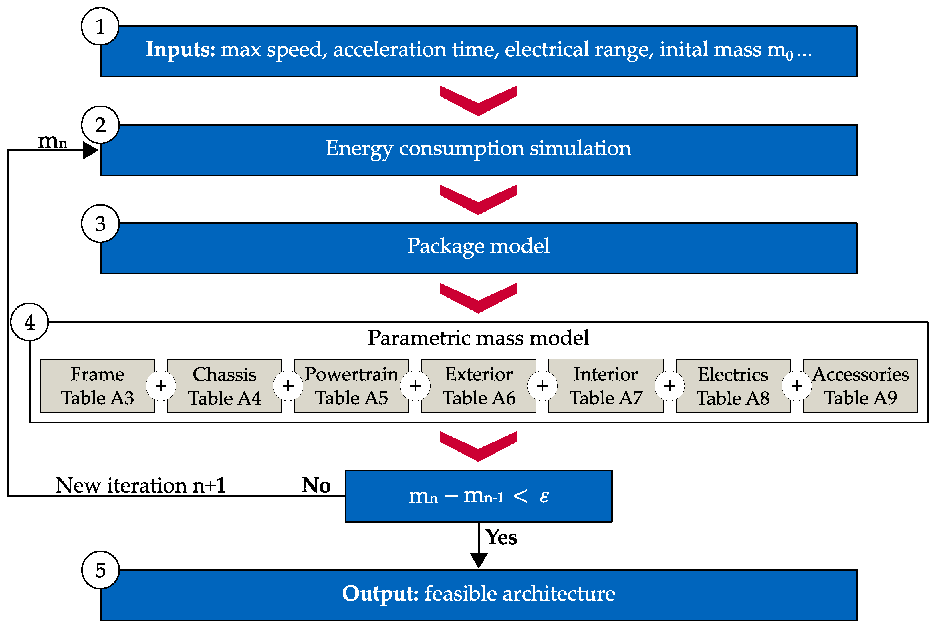
Volkswagen	up! e-up! (November 2013–June 2016)	e-Up!

). To assess parametric mass model accuracy alone, the vehicle package is not simulated and the energy consumption simulation is not applied (Figure 3). Therefore, the mass estimation presented in this section relies solely on the set of empirical models listed in Table A3, Table A4, Table A5, Table A6, Table A7, Table A8 and Table A9. Nevertheless, since the results of package modeling and energy consumption simulation are also required for mass modeling, we must collect further inputs to enable a standalone run of the parametric mass model. For example, the mass of the electric machine (Table A5) is calculated from its maximum torque, which we collect from the ADAC database [36].

A further required input is vehicle gross mass m_{veh, gross}, which is needed to calculate m_BIW (Table A3) as well as several subsystems of the chassis (Table A4). The ADAC database [36] also lists the gross mass m_{veh, gross} of every documented vehicle. To do this, we link each of the A2mac1 vehicles listed in Table 2, with the corresponding model series in ADAC and retrieve the gross mass of the heaviest model variant. Some vehicles, such as the Tesla Model 3 Long Range RWD, are not available in Europe and not documented in the ADAC database. In these cases, we retrieve the m_{veh, gross} from the manufacturer sites.

The BMW i3 120 Ah RE is a special case due to its range extender. With this vehicle, it is not possible to estimate the mass of the combustion engine, since internal combustion powertrains are not considered in the parametric mass model. Therefore, we simulate the vehicle as if it was built without the range extender.

Once the required inputs are collected, the vehicles in Table 2 are simulated and the mass of the seven modules estimated. For each simulated vehicle, we can then retrieve the real module masses from the A2mac1 database. Again, in the case of the BMW i3, we subtract the contributions of the combustion powertrain from the real powertrain mass listed in A2mac1, since we cannot simulate this subsystem.

Once the simulated and real module masses are available, we assess the correctness of the model using mean absolute error (MAE) and normalized mean absolute error (nMAE).

The resulting MAE and nMAE are shown in

Table 3. Overview of the MAE and nMAE for the different modules.

	Frame	Chassis	Powertrain	Exterior	Interior	Electrics	Accessories
MAE	19.12 kg	18.25 kg	37.45 kg	12.58 kg	17.80 kg	14.26 kg	2.73 kg
nMAE	5.7%	5.9%	6.0%	5.0%	8.3%	15.9%	28.4%

while Figure 5 depicts the deviation (in kg) between calculated and real modules masses. The powertrain module has the highest MAE, and the mean deviation between calculated and real powertrain masses is equal to 37 kg. This is because in most vehicles it is the heaviest module. For example, in BEVs such as the Audi e-tron [37] or the Opel Ampera-e [38], the battery accounts for more than 25% of the empty vehicle mass.

The powertrain of the Mercedes EQC has the highest deviation (red cross at −144 kg, Figure 5). Nevertheless, this deviation is not an error of the model, but is rather caused by the unconventional design of the battery. The EQC has massive battery housing with a series of internal side reinforcements [39], which lead to an above-average battery mass. Further inaccuracies occur with Tesla vehicles, whose electric machines have an above-average torque-to-mass ratio, which results in overestimation of these components.

With the other modules, the nMAE is usually between 5% and 8%. The electrics and accessories modules have higher values (15.9% and 28.4%, respectively). Nevertheless, these modules are lighter than the others, which means that the absolute error is not particularly high (compare the MAEs in Table 3 and the boxplots in Figure 5).

Overall the median of the absolute deviation is always close to 0 kg (Figure 5) which denotes that there is no tendency to over- or underestimate any of the seven modules.

Finally, for each vehicle in Table 2 the calculated empty vehicle mass (derived by totaling the contributions of the calculated modules) is compared with the real mass (Figure 6). The nMAE of the empty vehicle mass estimation shown in Figure 6 is 2.9%. This corresponds to a mean error of 53.1 kg for the evaluation dataset. This evaluation step confirms that, despite the limited amount of inputs, the mass estimation is still precise.

In the following section, the parametric mass model is applied in an assessment of the lightweight potential of current BEVs.

4. Lightweight Potential Assessment

To assess the lightweight potential, we define four reference vehicles (RVs) to be used in a parametric study (Table 4). The RVs come from different segments and have differing cells, topologies, and powertrain requirements.

The RV-A is a hatchback and has the same external dimensions as a BMW i3. It is fitted with a permanent magnet synchronous machine (PMSM) on its rear axle, while its battery (composed of prismatic cells) yields an electric range of 280 km. Like the BMW i3, the RV-A has a light BIW, which is assumed to be made entirely of aluminum (since carbon-fiber BIWs are not considered in the parametric mass model). Due to its aluminum frame and the small external dimensions, the RV-A is the lightest of the reference vehicles.

The RV-B is slightly larger than the RV-A and is derived from the VW ID.3. The battery consists of pouch cells and provides an electric range of 420 km. Machine topology and body type are the same as for the RV-A, but the RV-B has a lower drag coefficient of 0.26, like the VW ID.3 [40].

Table 4. Selected key characteristics of the RVs’ portfolios.

	RV-A	RV-B	RV-C	RV-D
Similar model	BMW i3 120 Ah	Volkswagen ID.3	Tesla Model 3 SR	Audi e-tron 55
Wheelbase (L101)	2570 mm	2770 mm	2875 mm	2928 mm
Width (W103)	1775 mm	1809 mm	1850 mm	1935 mm
Height (H100)	1570 mm	1568 mm	1443 mm	1629 mm
Body Type	Hatchback	Hatchback	Sedan	SUV
Drag coefficient	0.29	0.26	0.23	0.29
E-machine front/E-machine rear	–/PMSM	–/PMSM	–/PMSM	PMSM/PMSM
Cell type	Prismatic	Pouch	Cylindrical	Pouch
Acceleration time (0–100 km/h)	7.3 s	7.9 s	5.6 s	5.7 s
Maximum speed	150 km/h	160 km/h	225 km/h	200 km/h
Target range (in WLTP *)	280 km	420 km	400 km	400 km

* For the calculation of the target range we employ the Worldwide harmonized Light vehicles Test Procedure (WLTP). This procedure was developed by the UNECE in substitution of the obsolete New European Driving Cycle (NEDC) [41] and is adopted for type approval of light duty motor vehicles in Europe [42].

Table 4. Selected key characteristics of the RVs’ portfolios.

	RV-A	RV-B	RV-C	RV-D
Similar model	BMW i3 120 Ah	Volkswagen ID.3	Tesla Model 3 SR	Audi e-tron 55
Wheelbase (L101)	2570 mm	2770 mm	2875 mm	2928 mm
Width (W103)	1775 mm	1809 mm	1850 mm	1935 mm
Height (H100)	1570 mm	1568 mm	1443 mm	1629 mm
Body Type	Hatchback	Hatchback	Sedan	SUV
Drag coefficient	0.29	0.26	0.23	0.29
E-machine front/E-machine rear	–/PMSM	–/PMSM	–/PMSM	PMSM/PMSM
Cell type	Prismatic	Pouch	Cylindrical	Pouch
Acceleration time (0–100 km/h)	7.3 s	7.9 s	5.6 s	5.7 s
Maximum speed	150 km/h	160 km/h	225 km/h	200 km/h
Target range (in WLTP *)	280 km	420 km	400 km	400 km

* For the calculation of the target range we employ the Worldwide harmonized Light vehicles Test Procedure (WLTP). This procedure was developed by the UNECE in substitution of the obsolete New European Driving Cycle (NEDC) [41] and is adopted for type approval of light duty motor vehicles in Europe [42].

The RV-C is a sedan car, similar to the Tesla Model 3 Standard Range. It has a PMSM on the rear axle, and its battery is composed of cylindrical cells. The vehicle has demanding powertrain requirements (low acceleration time and high maximum speed) and a low drag coefficient. Although the RV-C is larger than the RV-B, it has a lower range requirement and lower consumption (also due to its improved aerodynamics). This results in a similar mass to the RV-B, despite the bigger dimensions.

Finally, the RV-D is similar to an Audi e-tron. It has an all-wheel-drive topology with a PMSM on each axle. While all the other vehicles have a rectangular battery installed beneath the passenger compartment, the RV-D has an additional level of cell modules underneath the second row of seats. This solution enables it to attain an electric range of 400 km, despite its large dimensions, high drag resistance, and mass.

The RVs are simulated with the vehicle architecture tool. The tool confirms the feasibility of all the RVs and yields the vehicle empty mass m_{veh,empty base}, which represents the mass of the vehicle when no lightweight measures are applied.

To study the impact of lightweight measures on the RVs, two mass savings (indicated as m_LW) of 50 kg and 100 kg are introduced and the RVs simulated again. Since the m_LW act like a PMS, they lead to further savings, according to the mass spiral shown in Figure 2. Despite the mass reduction, the RV portfolios (target range, acceleration time, maximum speed, Table 4) remain unchanged.

Table 5. Influence of different lightweight measures on energy consumption, required battery energy, and module masses.

Variable		RV-A	RV-B	RV-C	RV-D
Energy consumption (in WLTP)	mLW = 0 kg	14.75 kWh/100 km	14.63 kWh/100 km	14.16 kWh/100 km	19.31 kWh/100 km
	mLW = 50 kg	14.37 kWh/100 km	14.25 kWh/100 km	13.83 kWh/100 km	18.97 kWh/100 km
	mLW = 100 kg	13.99 kWh/100 km	13.97 kWh/100 km	13.42 kWh/100 km	18.60 kWh/100 km
Saved battery energy	mLW = 50 kg	1.22 kWh	1.80 kWh	1.84 kWh	1.51 kWh
	mLW = 100 kg	2.23 kWh	2.99 kWh	3.15 kWh	2.96 kWh
Saved machine power	mLW = 50 kg	7.12 kW	6.82 kW	8.68 kW	6.06 kW
	mLW = 100 kg	14.92 kW	12.35 kW	21.51 kW	16.66 kW
SMSs chassis module	mLW = 50 kg	9.63 kg	6.64 kg	3.22 kg	3.62 kg
	mLW = 100 kg	15.16 kg	10.74 kg	11.16 kg	6.83 kg
SMSs frame module	mLW = 50 kg	5.92 kg	7.86 kg	5.29 kg	5.82 kg
	mLW = 100 kg	12.14 kg	11.38 kg	11.15 kg	10.98 kg
SMSs powertrain module	mLW = 50 kg	9.45 kg	10.38 kg	12.89 kg	14.79 kg
	mLW = 100 kg	21.11 kg	22.24 kg	24.14 kg	24.33 kg
Total SPR	mLW = 50 kg	0.50	0.50	0.43	0.48
	mLW = 100 kg	0.48	0.44	0.46	0.42
Lightweight potential *	mLW = 50 kg	374 €	447 €	466 €	375 €
	mLW = 100 kg	691 €	750 €	874 €	782 €
Lightweight potential per kg *	mLW = 50 kg	7.48 €/kg	8.94 €/kg	9.32 €/kg	7.50 €/kg
	mLW = 100 kg	6.91 €/kg	7.50 €/kg	8.74 €/kg	7.82 €/kg

* Reduction of production costs due to savings in component dimensioning using the cost assumption specified in [43].

shows the impact of m_LW on energy consumption. The value listed at m_LW = 0 kg corresponds to the consumption of the vehicle without lightweight measures. The values listed at m_LW = 50 kg and m_LW = 100 kg represent the resulting energy consumption after the lightweight measure is applied and the SMSs calculated. The lightweight measure and its induced SMSs result in the RVs becoming lighter, which leads to a reduction in their energy consumption. The reduction in energy consumption depends on the selected test procedure for the target range definition. In the scope of this paper, we refer to the WLTP since it is the adopted procedure for type approval of light duty vehicles in Europe.

As the energy consumption decreases, less battery energy is needed to achieve the target range given in Table 4. For a 50 kg mass saving, the battery energy can be reduced by up to 1.84 kWh, while for 100 kg, the figure is between 2.33 kWh and 3.27 kWh. Due to the lower energy requirement, the battery can be downsized, which leads to mass savings in the powertrain and other module. These mass reductions also lower the machine power required, since with a lighter vehicle, less machine torque is needed to achieve the acceleration time.

Table 5 also shows a breakdown of the SMSs for chassis, frame, and powertrain. As it can be seen, the SMS are not continuous. For example, the RV-D has a lower SMS for the chassis than the other vehicles. This is due to the fact that despite the lightweight measure, the RV-D is still too heavy to reduce its wheel size. On the other hand all the other RVs can reduce their tire widths as a consequence of the lightweight measure thus generating higher SMS on the chassis.

The powertrain module always generates the highest SMSs. Finally, by adding the contributions of the three modules, it is possible to derive both the total SMSs induced by the m_LW and, in turn, the SPR. The SPR (regardless of the RVs and the m_LW) is within the range 0.42 to 0.50. This means that, on average, for each kilogram saved in the vehicle, a further saving of between 0.42 kg and 0.50 kg can be obtained on the basis of the SMSs.

Once the SPR and SMSs have been calculated, the lightweight potential of the RVs can be assessed. To do this, we use the cost data presented by König et al. [43]. First, based on the battery energy saved, we derive the saved battery cost by assuming an average cost at the pack level of 200 €/kWh for the year 2020 [43]. Furthermore, we assume production costs for the frame and chassis (material + labor + depreciation) of 1.3 €/kg for steel and 5.3 €/kg for aluminum. The PMSM costs are estimated at 10 €/kW. The cost savings are shown at the bottom of Table 5. We would like to stress that the values given are production costs, which normally account for 60% of the selling price, excluding taxes [43]. Furthermore, besides the given production cost savings, the customer also benefits from lightweight measures by way of the vehicle’s reduced energy consumption. As electricity prices vary significantly by country, we do not calculate these costs.

An assessment of the lightweight potential yields a range of between 6.9 €/kg and 9.3 €/kg. This means that, regardless of the RVs, if the costs of a lightweight measure are below 6.9 €/kg, they will be compensated by the induced power and energy saving. On the other hand, lightweight measures above 9.3 €/kg are not balanced for any of the RVs. Therefore, although they still result in a reduction in vehicle energy consumption, this will be accompanied by an increase in production costs.

The parametric study highlights that, in the case of BEVs, besides the benefits of reduced energy consumption, lightweight measures can also induce a significant monetary saving. Since the values shown in Table 5 are calculated for a single vehicle, high production volumes can induce effects of scale, thus amplifying the savings in production costs.

5. Discussion

After illustrating the potential of mass savings in the vehicle development process (Section 1), we present a tool and a parametric mass model capable of estimating the lightweight potential of BEVs (Section 2). Section 3 then presents an evaluation of the parametric mass model, which shows a percentual error of 2.9% (corresponding to approximately 53 kg). These deviations are mostly caused by the limited amount of modeling parameters. The choice of the modeling parameter set is the result of a tradeoff between modeling precision and usability of the tool during the early development design. Increasing the number of parameters would lead to higher accuracies, but would also hinder the usage of the tool for the early development design.

Regarding the vehicle interiors and exteriors, inaccuracies are mostly caused by the fact that their masses do not exclusively depend on the vehicle dimensions, but also on the model variant and optional. The available optional features, in turn, vary between manufacturers, which hinders the empirical modeling of this feature.

Inaccuracies are still present in the chassis because the subsystems of this module are sometimes built into different model series. This complicates the modeling since it is not always possible to precisely identify the model (and therefore the gross mass) that has been used for sizing the chassis subsystems. Regarding the powertrain, distinguishing between machine technologies (PMSM and IM) improved the results. Nevertheless, the number of machines available on the market is still low and displays a high variability between manufacturers. For a more precise estimation, it is possible to use sophisticated machine design tools such as [44]. However, such solutions require a higher number of input parameters, which are often not available in the early development phase.

Breaking the battery down into housing, module, and electrics components also improves the model accuracy, although deviations can still be observed, mostly in the battery housing. Finally, inaccuracies in the empty mass estimation are also caused by the fact that some vehicles are simply designed better than others and act therefore as outliners.

Following the mass model evaluation, we assess the lightweight potential of four RVs (Section 4). It is not possible to define an exact SPR but only a range, since there are components in the mass model which cause discontinuities. One example are the tires: as the vehicle mass decreases, the tire load and, in turn, the required tire volume also decreases. However, there are only a finite number of compatible tires, meaning that the SMSs caused by the tires are stepwise and not continuous [13].

6. Conclusions and Outlook

The parametric study yields an SPR between 0.42 and 0.50. Since the RVs cover different vehicle segments and have different portfolios, we assume that the derived SPR range can be generalized onto the majority of BEVs. Furthermore, since the gravimetric and volumetric energy density of lithium-ion batteries is expected to increase constantly in the coming years [43], this will lead to a decrease in SMSs caused by the battery and, in turn, of the SPR. Therefore, when quantifying lightweight potential, it is also necessary to carefully determine the year for which the as yet undeveloped vehicle is planned and choose the energy density accordingly.

A lightweight potential of between 6.9 €/kg and 9.3 €/kg is derived from the calculated SMSs and SPR. Again, it is possible to define a range (and not an exact value) for the lightweight potential. Nevertheless, the range can be applied to quantifying the suitability of lightweight measures during the vehicle development process. In Table 5, we also list the corresponding mass, power, and energy savings. Therefore, if more precise cost data is available, the lightweight potential can be recalculated using the data in Table 5.

The lightweight potential range given in this paper is only valid if every module and component is available for resizing. Since the tool is employable in the early development phase, there is still great design freedom, and resizing and adjustments are not as cost-intensive as in the following development phases. Nevertheless, this design freedom could be limited already in the early development if the vehicle has to be built on a preexisting platform (with an already given set of possible electric machines and cell sizes).

In conclusion, the method presented here is capable of estimating both SMSs and lightweight potential for BEVs. This approach can support manufacturers’ efforts to quantify lightweight measures and assist their decision-making in the early stages of the development process. In future publications, we will apply the presented tool to test the influence of other variables (such as acceleration time, drag coefficient, etc.) on vehicle energy consumption.