Optimization Control Strategy for Large Doubly-Fed Induction Generator Wind Farm Based on Grouped Wind Turbine

Abstract

This paper proposes a grouped, reactive power optimization control strategy to maximize the active power output of a doubly-fed induction generator (DFIG) based on a large wind farm (WF). Optimization problems are formulated based on established grouped loss models and the reactive power limits of the wind turbines (WTs). The WTs in the WF are grouped to relieve computational burden. The particle swarm optimization (PSO) algorithm is applied to optimize the distribution of reactive power among groups, and a proportional control strategy is used to distribute the reactive power requirements in each group. Furthermore, the proposed control strategy optimizes the reactive power distribution between the stator and the grid side converter (GSC) in each WT. The proposed control strategy greatly reduces the number of variables for optimization, and increases the calculation speed of the algorithm. Thus, the control strategy can not only increase the active power output of the WF but also enable the WF to track the reactive power dispatching instruction of the power grid. A simulation of the DFIG WF is given to verify the effectiveness of the proposed control strategy at different wind speeds and reactive power references.

1. Introduction

With the decline in global, non-renewable energy reserves and the increasingly serious problem of environmental pollution, the development and utilization of new energy represented by wind energy has become the general trend [1]. As more and more WFs are integrated into the power system, the reactive power control of WFs has become an important current issue to be faced [2,3]. With higher controllability, smaller converter capacity, and faster reactive power adjustment speed, DFIGs are widely used in WFs [4,5]. Furthermore, DFIGs can perform decoupling control of active and reactive power separately without the need of adding additional reactive power compensation sources, which is more economical and reliable [6,7].

The stator side of a DFIG is directly connected to the power grid, and the rotor side is connected to the power grid through a back-to-back PWM converter. The converter controls the rotor excitation current to realize the power transmission from the stator side to the power grid [8]. Therefore, the losses of the wind power system based on the DFIG consist of friction losses, core losses, copper losses, and converter losses. At present, most of the DFIG wind power generation systems are required to operate at a unit power factor state, which is a waste of their reactive power adjustment capability, especially at lower wind speeds. In order to solve this problem, the authors of [9] allocated the total reactive power requirements of the power grid in proportion to the reactive capacity of each WT. This can enable the WF to track the reactive power dispatching instruction of the power grid under the premise of the limit of the reactive power capacity of the WTs. However, the losses WFs are not considered in this method. A copper loss minimization control strategy for DFIG WFs is proposed in [10]. This minimizes the copper losses of WTs by allocating the reactive power between the stator and rotor of WTs. To minimize transmission line losses and transformer losses of a WF, an improved PSO algorithm is used to distribute reactive power among the WTs [11,12]. However, the WTs’ losses and converter losses are not considered, and they are a large part of the total losses of a WF. Furthermore, minimizing the transmission line losses and transformer losses may increase the converter losses. Reference [13] used a sequential quadratic programming method to optimize the reactive power distribution of a WF under constraints, which can effectively reduce the total losses of the WF.

To ensure that all node voltages are in a stable range, a model predictive control algorithm is proposed to implement the reactive power control of the WF [14]. Reference [15] uses the consistency protocol to allocate the reactive power among WTs, which can eliminate the steady state voltage error of WFs and provide a fast response for the system. A novel active power dispatching strategy based on dynamic grouping of WTs is proposed to obtain smoother active power references in [16]. This can enable WTs to track the dispatching instruction and alleviate the fatigue of WTs in order to achieve the reactive power requirements of the power grid and decrease the losses of the WF. The fatigue loads of wind turbine (WT) components are considered in [17] to achieve high active power output.

The control strategies mentioned above can reduce the losses of the WF and achieve the reactive power requirement of the power grid. However, the number of variables for optimization is larger. As a result, the computation burden is serious, and the control period must be long, which may weaken the optimization effect, especially in large WFs. Reference [18] proposes a distributed optimization method based on ADMM, which distributes the calculation work to each unit, but has high requirements for real-time communication. References [19,20] propose a hierarchical optimization strategy by decomposing the optimization objective into two levels: wind turbine optimization and wind farm optimization, thus simplifying the optimization algorithm to a certain extent. Although, when the scale of the wind farm is large, the calculation will still be more complex.

Therefore, this paper proposes a grouped reactive power optimization control strategy for large DFIG WFs, which is partly reported in PESA [21]. It divides the WTs into several groups and uses the PSO algorithm to optimize the distribution of reactive power among groups. Then, the reactive power requirements are distributed to each WT within each group by a proportional optimization strategy. The proposed control strategy greatly reduces the number of variables for optimization and increases the calculation speed of the algorithm. As a result, it reduces the total losses of the WF and increases the active power output of the WF. Meanwhile, the WF with the proposed control strategy can track the reactive power dispatching instruction of the power grid.

The paper is organized as follows. Section 2 presents the losses model of the WF. Section 3 discusses the proposed grouped optimization control strategy. The effect of the proposed strategy is analyzed in Section 4. Finally, Section 5 concludes with the contribution of this paper.

2. Losses Model of the Wind Farm

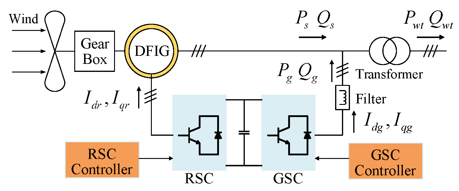
2.1. Losses Model of the DFIG

The basic configuration of the DFIG is shown in Figure 1.

The losses of the DFIG consist of friction losses, core losses, and copper losses. The first two losses can be considered constant under a certain operation point [10]. Therefore, only copper losses are considered in this paper, which can be described by [22]

$$\begin{array}{c} P_{\mathit{cu}}^{\mathit{loss}}{=R}_s{(I}_{\mathit{ds}}^2{+I}_{\mathit{qs}}^2{)+R}_r{(I}_{\mathit{dr}}^2{+I}_{\mathit{qr}}^2)\end{array}$$

(1)

where R_s and R_r are the equivalent resistances of the stator and rotor winding, respectively; I_ds and I_qs are the d-axis and q-axis components of the stator current; I_dr and I_qr are the d-axis and q-axis components of the rotor current, respectively.

The losses of the converter can be represented by the following equation [23]

$$\begin{array}{c} P_{\mathit{con}}^{\mathit{loss}}{=P}_c{+R}_c\left(I^{m^2}{ - c}_0^2\right)\end{array}$$

(2)

where $I^m$ is the root mean square (RMS) value of the sinusoidal current at the converter alternating current terminal. P_c, R_c, and c₀ are selected by

$$\begin{array}{c} \left\{\begin{array}{c}{P}_c{=0, R}_c=7{.9 \times 10}^{-4}{, c}_0{=0 I}^m \le 0.17\\ P_c=2{.7 \times 10}^{-5}{, R}_c=2{.9 \times 10}^{-4}{, c}_{0 }=0.17 0{.17 < I}^m \le 0.52\\ P_c=1{.2 \times 10}^{-4}{, R}_c=2{.2 \times 10}^{-4}{, c}_0=0.52 0{.52 < I}^m \le 1\end{array}\right.\end{array}$$

(3)

Therefore, the losses of the rotor side converter (RSC) $P_{\mathit{RSC}}^{\mathit{loss}}$ and the losses of the GSC $P_{\mathit{GSC}}^{\mathit{loss}}$ can be expressed by

$$\begin{array}{c} \left\{\begin{array}{c}{P}_{\mathit{RSC}}^{\mathit{loss}}{=P}_{\mathrm{cr}}{+R}_{\mathrm{cr}}{(I}_{\mathit{RSC}}^m{}^2 {- c}_r^2)\\ P_{\mathit{GSC}}^{\mathit{loss}}{=P}_{\mathrm{cg}}{+R}_{\mathrm{cg}}{(I}_{\mathit{GSC}}^m{}^2 {- c}_g^2)\end{array}\right.\end{array}$$

(4)

where $I_{\mathit{RSC}}^m$ is the RMS value of sinusoidal current from the RSC to the power grid, and $I_{\mathit{GSC}}^m$ is the RMS value of sinusoidal current from the GSC to the generator. They can be calculated by

$$\begin{array}{c} \left\{\begin{array}{c}{I}_{\mathit{RSC}}^m=\sqrt{I_{\mathit{dr}}^2{+I}_{\mathit{qr}}^2}\\ I_{\mathit{GSC}}^m=\sqrt{I_{\mathit{dg}}^2{+I}_{\mathit{qg}}^2}\end{array}\right.\end{array}$$

(5)

where $I_{\mathit{dg}}$ and $I_{\mathit{qg}}$ are the d-axis and q-axis components of the GSC current, respectively.

The losses of the grid side filter are given by

$$\begin{array}{c} P_{\mathit{fil}}^{\mathit{loss}}{=R}_{\mathit{fil}}(I_{\mathit{dg}}^2 {+I}_{\mathit{qg}}^2)\end{array}$$

(6)

where $R_{\mathit{fil}}$ is the equivalent resistance of the filter.

The total losses of the DFIG wind power generation system $P_{\mathit{wt}}^{\mathit{loss}}$ can be expressed by,

$$\begin{array}{c} P_{\mathit{wt}}^{\mathit{loss}}{=P}_{\mathit{cu}}^{\mathit{loss}}{+P}_{\mathit{RSC}}^{\mathit{loss}}{+P}_{\mathit{GSC}}^{\mathit{loss}}{+P}_{\mathit{fil}}^{\mathit{loss}}\end{array}$$

(7)

2.2. Losses Model of Transmission Network

The cable model of the transmission network is shown in Figure 2 where P₁ + jQ₁ represents the power flowing away from node 1 to node 2; V₁ represents the voltage of node 1; R + jX represents the complex impedance of the cable between node 1 and node 2.

The losses of the cable are calculated by

$$\begin{array}{c} P_{\mathit{cable}}^{\mathit{loss}}=\frac{P_1^2{+Q}_1^2}{V_1^2} R\end{array}$$

(8)

The active power losses of the transformer are calculated by

$$\begin{array}{c} P_{\mathit{tran}}^{\mathit{loss}}{=P}_0+{\beta }^2{P}_k\end{array}$$

(9)

where $\beta$ is the load ratio of the transformer; $P_0$ and $P_k$ are the no-load losses and load losses of the transformer, respectively.

The transmission losses include the cable losses and transformer losses, which can be expressed by

$$\begin{array}{c} P_{\mathit{net}}^{\mathit{loss}}{=P}_{\mathit{cable}}^{\mathit{loss}}{+P}_{\mathit{tran}}^{\mathit{loss}}\end{array}$$

(10)

As a result, the total losses of the WF can be calculated by

$$\begin{array}{c} P_{\mathit{wf}}^{\mathit{loss}}{=P}_{\mathit{wt}}^{\mathit{loss}}{+P}_{\mathit{net}}^{\mathit{loss}}\end{array}$$

(11)

3. Grouped Optimization Control Strategy

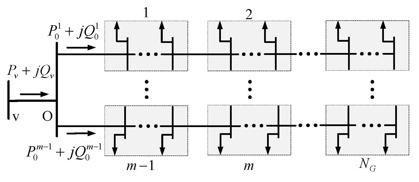
3.1. Configuration of a WF

The typical configuration of a WF is shown in Figure 3. The WF is connected to the power grid with a boost transformer. The transformer connects many feeder lines through a collector bus. Each feeder is composed of a plurality of WTs placed with equal distance.

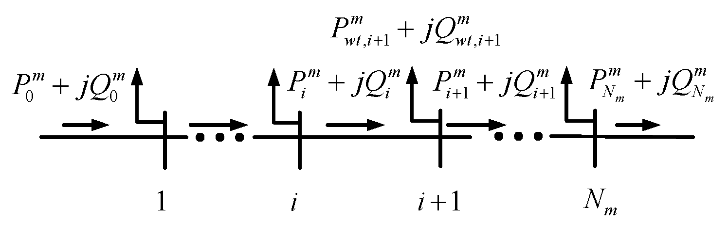
3.2. Power Flow Model of a WF

The grouped power flow model of the DFIG WF is shown in Figure 4. The direction from the power grid to the WT is defined as a positive power flow.

The WTs in the WF are divided into N_G groups, and each group contains N_m WTs, where m = 1, 2, ..., N_G. Node v is a slack bus node, and node O is a collector bus node. Node 0 of group m + 1 is the last node of group m. $P_v$ + ${\mathit{jQ}}_v$ is the power flowing away from node v to node O; $P_0^1{+\mathit{jQ}}_0^1$ is the power flowing away from the node O to the group 1. $P_0^{m-1}{+\mathit{jQ}}_0^{m-1}$ is the power flowing away from node O to the group m − 1.

The power flow model of group m is shown in Figure 5. The positive direction of power flow is consistent with that of the WF.

3.3. Objective Function

Maximizing the active power output of a DFIG WF is a global optimization problem with constraints. This includes power balance constraints, power grid reactive power dispatching constraints, the voltage constraints, and DFIG rated power constraints. Based on the grouped power flow model, the objective function for maximizing the active power output of the WF can be expressed by

$$\begin{array}{c} f =\underset{P,Q,V}{\mathit{max}}\left\{{\displaystyle {\displaystyle \sum }_{m=1}^{N_G}}{\displaystyle {\displaystyle \sum }_{i=1}^{N_m}}\left(P_{\mathit{wt},i}^m - P_{\mathit{wt},i}^{m,\mathit{loss}}{- P}_{\mathit{tran},i}^{m,\mathit{loss}} {- R}_{i-1}^m{I}_{i-1}^m{}^2\right){- R}_v{I}_v^2\right\}\end{array}$$

(12)

$$\begin{array}{c} \left\{\begin{array}{c}{P}_{i+1}^m{=P}_i^m {- P}_{\mathit{wt},i}^m {- R}_i^m{I}_i^m{}^2\\ Q_{i+1}^m{=Q}_i^m {- Q}_{\mathit{wt},i}^m {- X}_i^m{I}_i^m{}^2\\ V_{i+1}^m{}^2{=V}_i^m{}^2 - 2\left(R_i^m{P}_i^m {- X}_i^m{Q}_i^m\right){+I}_i^m{}^2\left({\left(R_i^m\right)}^2+{\left(X_i^m\right)}^2\right)\end{array}\right.\end{array}$$

(13)

$$\begin{array}{c}{ V}_O^2{=V}_v^2 - 2\left(R_v{P}_v {- X}_v{Q}_v\right){+I}_v^2\left(R_v^2 {+X}_v^2\right)\end{array}$$

(14)

$$\begin{array}{c}{ P}_{N_m}^{N_G}{=0, Q}_{N_m}^{N_G}=0 \end{array}$$

(15)

$$\begin{array}{c}{ Q}_v{=Q}_{\mathit{wf}}^{\mathit{ref}}\end{array}$$

(16)

$$\begin{array}{c}{ V}_{\mathit{min} } \le { V}_i^m \le { V}_{\mathit{max} }\end{array}$$

(17)

$$\begin{array}{c}{ Q}_{\mathit{wt},i}^m{=Q}_{s,i}^m{+Q}_{g,i}^m\end{array}$$

(18)

$$\begin{array}{c} \left\{\begin{array}{c}{Q}_{\mathit{smin},i}^m \le { Q}_{s,i}^m \le { Q}_{\mathit{smax},i}^m\\ Q_{\mathit{gmin},i}^m \le { Q}_{g,i}^m \le { Q}_{\mathit{gmax},i}^m\end{array}\right.\end{array}$$

(19)

where m means the m^th group, $P_{\mathit{wt},i}^{m,\mathit{loss}}$ is the losses of the i^th WT, $P_{\mathit{tran},i}^{m,\mathit{loss}}$ is the losses of the i^th transformer. $R_i^m$ is the resistance of the cable between node i and node i + 1. $X_i^m$ is the reactance of the cable between node i and node i + 1. $I_i^m$ is the current flowing from node i to node i + 1. $V_i^m$ is the voltage of node i. $R_v$ and ${ X}_v$ are complex impedances of the cable between node v and node O. $V_v$ and $V_{O }$ are the voltages of node v and node O, respectively. $I_v$ is the current flowing from node v to node O. $I_i^m$ and $I_v$ can be calculated by Equation (20). $Q_{\mathit{wf}}^{\mathit{ref}}$ is the reference value of the total reactive power of the WF. $P_{N_m}^{N_G}{ \mathrm{and} Q}_{N_m}^{N_G}$ are the active power and reactive power flowing away from the last node of group $N_G$, respectively. In this paper, $V_{\mathit{max} }$ and ${ V}_{\mathit{min} }$ are the upper and lower limits of the node voltage, and they are assumed to be 0.90 p.u. and 1.1 p.u., respectively. $Q_{s,i}^m$ is the reactive power output of the stator of the i^th WT, and its lower and upper limits are $Q_{\mathit{smin},i}^m$ and $Q_{\mathit{smax},i}^m$, respectively. ${ Q}_{g,i}^m$ is the reactive power output of the GSC of the i^th WT, and its lower and upper limits are $Q_{\mathit{gmin},i}^m$ and $Q_{\mathit{gmax},i}^m$, respectively. They are calculated by Equations (21)–(23) [24].

$$\begin{array}{c} \left\{\begin{array}{c}{I}_i^m{}^2=\frac{{\left(P_i^m\right)}^2+{\left(Q_i^m\right)}^2}{{\left(V_i^m\right)}^2}\\ I_v^2=\frac{P_v^2{+Q}_v^2}{V_v^2}\end{array}\right.\end{array}$$

(20)

$$\begin{array}{c} \left\{\begin{array}{c}{Q}_{\mathit{smin},i}^m{=\min (Q’}_{\mathit{smin}},-\sqrt{S_s^2 {- P}_s^2})\\ Q_{\mathit{smax},i}^m{=\max (Q’}_{\mathit{smax}},\sqrt{S_s^2 {- P}_s^2})\end{array}\right.\end{array}$$

(21)

$$\begin{array}{c} \left\{\begin{array}{c}{Q’}_{\mathit{smin}}=-\frac{{3V}_s^2}{{2X}_s} - \sqrt{{\left(\frac{{3X}_m}{{2X}_s}{V}_s{I}_{\mathrm{rmax}}\right)}^2 {- P}_s^2}\\ {Q’}_{\mathit{smax}}=-\frac{{3V}_s^2}{{2X}_s}+\sqrt{{\left(\frac{{3X}_m}{{2X}_s}{V}_s{I}_{\mathrm{rmax}}\right)}^2 {- P}_s^2}\end{array}\right.\end{array}$$

(22)

$$\begin{array}{c} \left\{\begin{array}{c}{Q}_{\mathit{gmin},i}^m=-\sqrt{S_{g }^2{- P}_g^2}\\ Q_{\mathit{gmax},i}^m=\sqrt{S_g^2 {- P}_g^2}\end{array}\right.\end{array}$$

(23)

where $S_s$ is the rated capacity of the stator winding; P_s is the active power output of the WT; V_s is the stator voltage of the WT; X_s is the reactance of stator winding. $X_m$ is the excitation reactance of the WT; I_rmax is the maximum current of the RSC; $S_g$ is the capacity of the GSC, and $P_g$ is the active power of the GSC.

The constraints will be eliminated if it is included on the objective function. Therefore, penalty function y is added to the objective function instead of the constraints. The active power output of the WTs are assumed to be equal to their wind powers in this paper. Therefore, $P_{\mathit{wt},i}^m$ can be regarded as a constant parameter, and it isn’t considered in the objective function. Because the reactive power allocated by the proportional control strategy will not exceed the reactive capacity of the WTs in each group, Equation (19) is replaced by Equation (25). Then, the objective function can be formulated as a grouped optimization problem by

$$\begin{array}{c} F=\underset{Q_{s,i}^m{,Q}_{g,i}^m}{\mathit{min}}\left\{{\displaystyle {\displaystyle \sum }_{m=1}^{N_G}}{\displaystyle {\displaystyle \sum }_{i=1}^{N_m}}\left(P_{\mathit{wt},i}^{m,\mathit{loss}}{+P}_{\mathit{tran},i}^{m,\mathit{loss}}{+R}_{i-1}^m{I}_{i-1}^m{}^2\right){+R}_v{I}_v^2+y\right\}\end{array}$$

(24)

Combining Equations (13)–(15) and (18), one yields

$$\begin{array}{c} \left\{\begin{array}{c}{Q}_{\mathit{Gsmin}}^m \le { Q}_{\mathit{Gs}}^m \le { Q}_{\mathit{Gsmax}}^m\\ Q_{\mathit{Ggsmin}}^m \le { Q}_{\mathit{Gg}}^m \le { Q}_{\mathit{Ggmax}}^m\end{array}\right.\end{array}$$

(25)

where

$$\begin{array}{c} y={\displaystyle {\displaystyle \sum }_{m=1}^{N_G}}{\displaystyle {\displaystyle \sum }_{i=1}^{N_m}}{y}_i^m{+y}_0\end{array}$$

(26)

$$\begin{array}{c} y_i^m=\left\{\begin{array}{c}{0; V}_{\mathit{min} } \le { V}_i^m \le { V}_{\mathit{max} }\\ {1 \times 10}^4{; V}_i^m {< V}_{\mathit{min}} \mathrm{or} V_i^m{ > V}_{\mathit{max} }\end{array}\right.\end{array}$$

(27)

$$\begin{array}{c} y_0=\left\{\begin{array}{c}{0; |Q}_{\mathit{wf}}^{\mathit{ref}} - Q_v| \le {\epsilon }_q\\ {1 \times 10}^4{; |Q}_{\mathit{wf}}^{\mathit{ref}} - Q_v| > {\epsilon }_q\end{array}\right.\end{array}$$

(28)

where ${\epsilon }_q$ is the accuracy of reactive power dispatching.

$Q_{\mathit{Gs}}^m$ and $Q_{\mathit{Gg}}^m$ are the sum of $Q_{s,i}^m$ and ${ Q}_{g,i}^m$ in group m, respectively. They can be calculated by Equation (29). $Q_{\mathit{Gsmax}}^m$ and $Q_{\mathit{Gsmin}}^m$ are the upper and lower limits of $Q_{\mathit{Gs}}^m$. $Q_{\mathit{Ggmax}}^m$ and $Q_{\mathit{Ggsmin}}^m$ are the upper and lower limits of $Q_{\mathit{Gg}}^m$. They can be calculated by Equation (30).

$$\begin{array}{c} \left\{\begin{array}{c}{Q}_{\mathit{Gs}}^m={\displaystyle {\displaystyle \sum }_{i=1}^{N_m}}{Q}_{s,i}^m\\ Q_{\mathit{Gg}}^m={\displaystyle {\displaystyle \sum }_{i=1}^{N_m}}{ Q}_{g,i}^m\end{array}\right.\end{array}$$

(29)

$$\begin{array}{c} \left\{\begin{array}{c}{Q}_{\mathit{Gsmax}}^m={\displaystyle {\displaystyle \sum }_{i=1}^{N_m}}{Q}_{\mathit{smax},i}^m{, Q}_{\mathit{Gsmin}}^m= {\displaystyle {\displaystyle \sum }_{i=1}^{N_m}}{Q}_{\mathit{smin},i}^m\\ Q_{\mathit{Ggmax}}^m={\displaystyle {\displaystyle \sum }_{i=1}^{N_m}}{Q}_{\mathit{gmax},i}^m{, Q}_{\mathit{Ggmin}}^m= {\displaystyle {\displaystyle \sum }_{i=1}^{N_m}}{Q}_{\mathit{gmin},i}^m\end{array}\right.\end{array}$$

(30)

3.4. Grouped Optimization Scheme

The block diagram scheme of grouped reactive power optimization control strategy for the DFIG WF is shown in Figure 6. Line parameters include the reactance and resistance of the cable. WT parameters include X_m, X_s, I_rmax, and $S_g$, etc. $Q_{\mathit{Gs}}^{m,\mathit{ref}}$ and $Q_{\mathit{Gg}}^{m,\mathit{ref}}$ are the reference values of $Q_{\mathit{Gs}}^m$ and $Q_{\mathit{Gg}}^m$, respectively. $Q_{s,i}^{m,\mathit{ref}}$ and $Q_{g,i}^{m,\mathit{ref}}$ are the reference values of $Q_{s,i}^m$ and ${ Q}_{g,i}^m$, respectively. $v_i^m$ is wind speed of the i^th WT in group m. After receiving the dispatching order, the controller substitutes the line and WT parameters into the objective function. Then, it uses the PSO algorithm to optimize the reactive power distribution among groups to obtain $Q_{\mathit{Gs}}^{m,\mathit{ref}}$ and $Q_{\mathit{Gg}}^{m,\mathit{ref}}$, and uses the proportional control strategy to distribute the reactive power requirements within each group to obtain $Q_{s,i}^{m,\mathit{ref}}$ and $Q_{g,i}^{m,\mathit{ref}}$.

3.5. Grouped Optimization Step

The terminology and formula used are the following:

$v_j$ represents the velocity of the j^th particle. x_j is the position of the j^th particle, and it represents a feasible solution of the objective function F. They are expressed by Equation (31) where subscript d represents dimensions, d = 1, 2, ..., ${2N}_G$.

$$\begin{array}{c} \left\{\begin{array}{c}{v}_j{=[v}_{j,1}{,\dots , v}_{j,d}{,\dots , v}_{{j,2N}_G}]\\ x_j{=[x}_{j,1}{,\dots , x}_{j,d}{,\dots , x}_{{j,2N}_G}\left]{=[Q}_{\mathit{Gs}}^1{,\dots , Q}_{\mathit{Gs}}^{N_G}{, Q}_{\mathit{Gg}}^1{,\dots , Q}_{\mathit{Gg}}^{N_G}\right]\end{array}\right.\end{array}$$

(31)

$v^{\mathit{max}}$ and $v^{\mathit{min}}$ are the maximum and minimum values of velocity of particles, respectively, $x^{\mathit{max}}$ and $x^{\mathit{min}}$ are the maximum and minimum values of the position of particles, respectively. They all have ${2N}_G$ dimensions.

Step 1: Divide the WTs of the WF into N_G groups, and calculate $Q_{\mathit{Gsmax}}^m$, $Q_{\mathit{Gsmin}}^m$, $Q_{\mathit{Ggmax}}^m$, $Q_{\mathit{Ggmin}}^m$, ${\mathit{scs}}_{s,i}^m$, and ${\mathit{scg}}_{g,i}^m$ according to Equations (30) and (33).

$$\begin{array}{c} \left\{\begin{array}{c}{\mathit{scs}}_{s,i}^m=\frac{Q_{\mathit{smax},i}^m}{{{\displaystyle \sum }}_{i=1}^{N_m}{Q}_{\mathit{smax},i}^m}\\ {\mathit{scg}}_{g,i}^m=\frac{Q_{\mathit{gmax},i}^m}{{{\displaystyle \sum }}_{i=1}^{N_m}{Q}_{\mathit{gmax},i}^m}\end{array}\right.\end{array}$$

(32)

where ${\mathit{scs}}_{s,i}^m$ and ${\mathit{scg}}_{g,i}^m$ are the proportion of stator reactive power and GSC reactive power of the i^th WT in group m.

Step 2: Initialize variables: the number of particles N_P, optimization accuracy ε, constant coefficient $c_1$ and $c_2$, dispatching accuracy ${\epsilon }_q$, the maximum and minimum values of the velocity of particles in each dimension $v^{\mathit{MAX}}$ and $v^{\mathit{MIN}}$.

Step 3: Initialize variables v_j and $x_j$(j = 1, 2, ..., N_P) according to

$$\begin{array}{c} \left\{\begin{array}{c}{v}_j{=v}^{\mathit{min}} {+r}_v{(v}^{\mathit{max}} {- v}^{\mathit{min}})\\ x_j{=x}^{\mathit{min}} {+r}_x{(x}^{\mathit{max}} {- x}^{\mathit{min}})\end{array}\right.\end{array}$$

(33)

where $r_v$ and $r_x$ are random numbers between 0 and 1. $v^{\mathit{max}}$, $v^{\mathit{min}}$, $x^{\mathit{max}}$, and $x^{\mathit{min}}$ are expressed by

$$\begin{array}{c} \left\{\begin{array}{c}{v}^{\mathit{max}}= \left[v^{\mathit{MAX}}{,\dots , v}^{\mathit{MAX}}{,\dots , v}^{\mathit{MAX}}\right] \\ v^{\mathit{min}}= \left[v^{\mathit{MIN}}{,\dots , v}^{\mathit{MIN}}{,\dots , v}^{\mathit{MIN}}\right]\\ x^{\mathit{max}}{=[Q}_{\mathit{Gsmax}}^1{,\dots , Q}_{\mathit{Gsmax}}^{N_G}{, Q}_{\mathit{Ggmax}}^1{,\dots , Q}_{\mathit{Ggmax}}^{N_G}] \\ x^{\mathit{min}}{=[Q}_{\mathit{Gsmin}}^1{,\dots , Q}_{\mathit{Gsmin}}^{N_G}{, Q}_{\mathit{Ggmin}}^1{,\dots , Q}_{\mathit{Ggmin}}^{N_G}]\end{array}\right.\end{array}$$

(34)

Step 4: Define ${\mathit{pbest}}_j$ = $x_j$, gbest = $\left[0, \dots , 0,\dots , 0\right]$. Where gbest has ${2N}_G$ dimensions. Decode variables according to Equation (36) and calculate $Q_{s,i}^m$ and $Q_{g,i}^m$ according to Equation (36). Then, calculate $F \left(x_j\right)$ and define ${\mathit{fpbest}}_j$ = $F \left({\mathit{pbest}}_j\right)$.

$$\begin{array}{c} {[Q}_{\mathit{Gs}}^1{,\dots , Q}_{\mathit{Gs}}^{N_G}{, Q}_{\mathit{Gg}}^1{,\dots , Q}_{\mathit{Gg}}^{N_G}] =x_j\end{array}$$

(35)

$$\begin{array}{c} \left\{\begin{array}{c}{Q}_{s,i}^m{=Q}_{\mathit{Gs},i}^m{\mathit{scs}}_{s,i}^m\\ Q_{g,i}^m{=Q}_{\mathit{Gg},i}^m{\mathit{scg}}_{g,i}^m\end{array}\right.\end{array}$$

(36)

Step 5: Find out the ${F(\mathit{pbest}}_j)$ with minimax value, and assign this value to $\mathit{fgbest}$. Meanwhile, assign the corresponding pbest_j to gbest.

Step 6: Update v_j according to Equation (37) where d = 1, 2, ..., ${2N}_G$. $r_1$ and $r_2$ are random numbers between 0 and 1.

$$\begin{array}{c} \left\{\begin{array}{c}{v}_j{=v}_j{+c}_1{r}_1\left({\mathit{pbest}}_j - x_j\right){+c}_2{r}_2\left(\mathit{gbest} - x_j\right)\\ v_{j,d}=\left\{\begin{array}{c}{v}^{\mathit{MAX}}{; v}_{j,d}{ > v}^{\mathit{MAX}}\\ v^{\mathit{MIN}}{; v}_{j,d}{ < v}^{\mathit{MIN}}\end{array}\right.\end{array}\right.\end{array}$$

(37)

Step 7: Update $x_j$ according to

$$\begin{array}{c} \left\{\begin{array}{c}{x}_j{=x}_j{+v}_j\\ x_{j,d}=\left\{\begin{array}{c}{x}_{j,d}^{\mathit{max}}{; x}_{j,d}{ > x}_d^{\mathit{max}}\\ x_{j,d}^{\mathit{min}}{; x}_{j,d}{ < x}_d^{\mathit{min}}\end{array}\right.\end{array}\right.\end{array}$$

(38)

Step 8: Decode variables according to Equation (35) and calculate $Q_{s,i}^m$ and $Q_{g,i}^m$ according to Equation (36). Calculate $F \left(x_j\right)$ and update ${\mathit{fpbest}}_j$ and ${\mathit{pbest}}_j$ according to

$$\begin{array}{c} \left\{\begin{array}{c}{\mathit{fpbest}}_j=\left\{\begin{array}{c}{\mathit{fpbest}}_j{; \mathit{fpbest}}_j \le F \left(x_j\right)\\ F \left(x_j\right){; \mathit{fpbest}}_j > F \left(x_j\right)\end{array}\right.\\ { \mathit{pbest}}_j=\left\{\begin{array}{c}{\mathit{pbest}}_j{; \mathit{fpbest}}_j \le F \left(x_j\right)\\ x_j{; \mathit{fpbest}}_j > F \left(x_j\right)\end{array}\right.\end{array}\right.\end{array}$$

(39)

Step 9: Update $\mathit{fgbest}$ and $\mathit{gbest}$ according to

$$\begin{array}{c} \left\{\begin{array}{c}\mathit{fgbest}=\left\{\begin{array}{c}{\mathit{fpbest}}_j{; \mathit{fpbest}}_j \le \mathit{fgbest}\\ {\mathit{fgbest}; \mathit{fpbest}}_j > \mathit{fgbest}\end{array}\right.\\ \mathit{gbest}=\left\{\begin{array}{c}{\mathit{pbest}}_j{; \mathit{fpbest}}_j \le \mathit{fgbest}\\ {\mathit{gbest}; \mathit{fpbest}}_j > \mathit{fgbest}\end{array}\right.\end{array}\right.\end{array}$$

(40)

Step 10: Repeat Steps 6–9 until the deviation between the two adjacent iterations is below $\epsilon$.

Step 11: Calculate $Q_{s,i}^{m,\mathit{ref}}$ and $Q_{g,i}^{m,\mathit{ref}}$ according to

$$\begin{array}{c} {[Q}_{\mathit{Gs}}^{1,\mathit{ref}}{,\dots , Q}_{\mathit{Gs}}^{N_G,\mathit{ref}}{, Q}_{\mathit{Gg}}^{1,\mathit{ref}}{,\dots , Q}_{\mathit{Gg}}^{N_G,\mathit{ref}}] =\mathit{gbest}\end{array}$$

(41)

$$\begin{array}{c} \left\{\begin{array}{c}{Q}_{s,i}^{m,\mathit{ref}}{=Q}_{\mathit{Gs},i}^{m,\mathit{ref}}{\mathit{scs}}_{s,i}^m\\ Q_{g,i}^{m,\mathit{ref}}{=Q}_{\mathit{Gg},i}^{m,\mathit{ref}}{\mathit{scg}}_{g,i}^m\end{array}\right.\end{array}$$

(42)

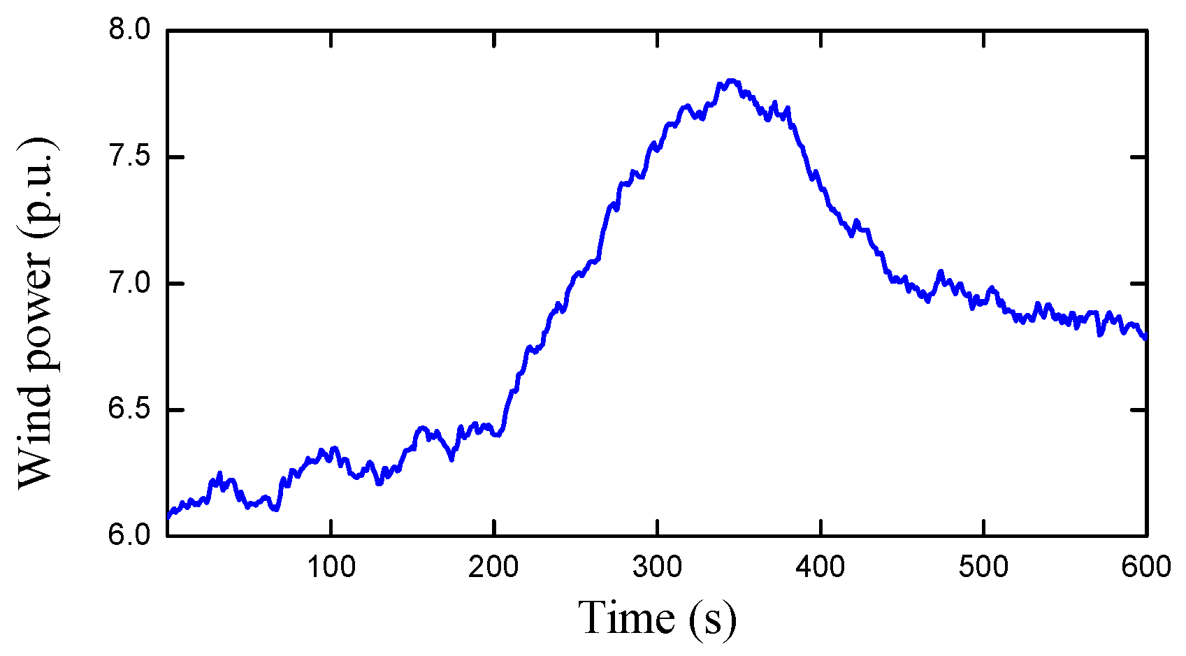
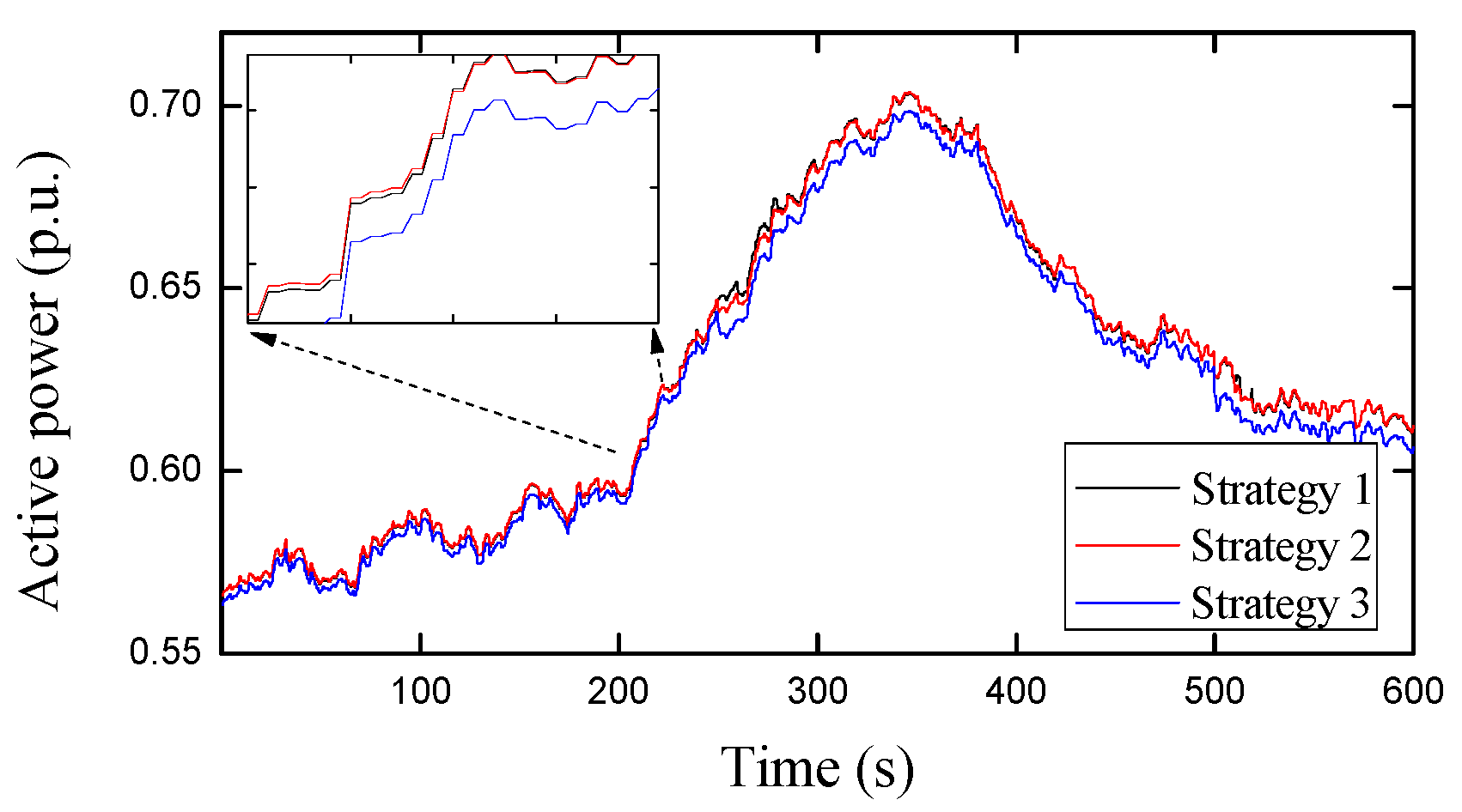
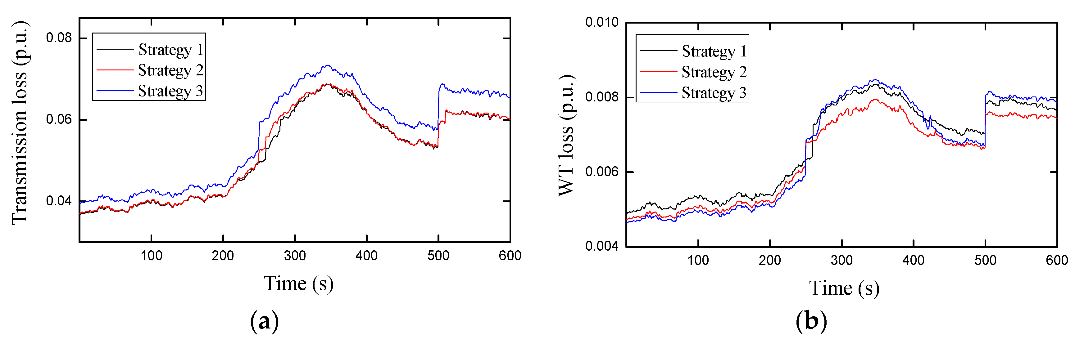
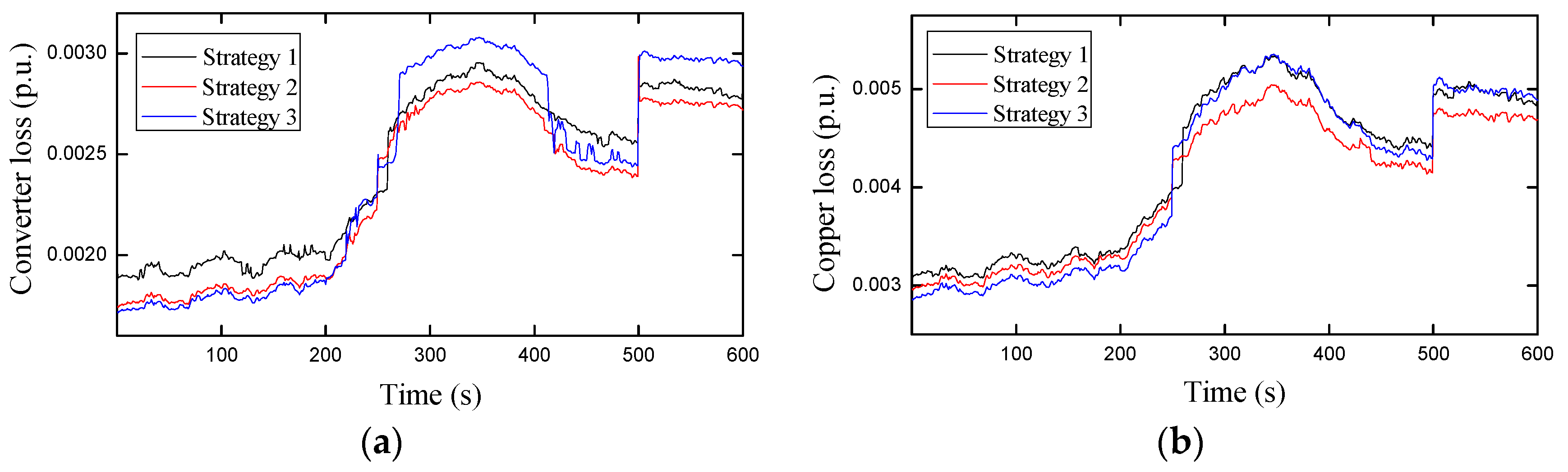
4. Simulation Results

In this paper, a simulated DFIG WF with two feeders was built on the MATLAB/Simulink. Where each feeder was composed of 10 × 5MW DFIG. The parameters are shown in

Table 1. Parameters of Grouped optimization strategy.

Parameters	Value
Particles number, NP	150
Reactive accuracy, ${\epsilon }_q$	0.01
Number of groups, NG	6
Optimization accuracy, ε	0.00001
Maximum velocity, $v^{\mathit{MAX}}$	0.1
Minimum velocity, $v^{\mathit{MIN}}$	−0.1
Constant coefficient, $c_1$	1.4961
Constant coefficient, $c_2$	1.4961

and

Table 2. Parameters of 5 MW DFIG.

Parameters	Value	Per Unit Value
Rated Mechanical Power	5 MW	0.05 p.u.
Rated stator voltage	690 V	0.017 p.u.
Stator Winding Resistance, Rs	1.552 mΩ	0.000142 p.u.
Rotor Winding Resistance, Rr	1.446 mΩ	0.000133 p.u.
Stator Leakage Reactance, Xs	2.033 Ω	0.1867 p.u.
Excitation reactance, Xm	1.733 Ω	0.1591 p.u.
Filter Resistance, Rfil	0.6791 mΩ	0.000062 p.u.
Rated WF Power, SWF	100 MVA	1.0 p.u.
Base Impedance, ZB	10.89 Ω	1.0 p.u.
Cable resistance, R	0.1 Ω/km	0.00918 p.u.
Cable reactance, X	0.129 Ω/km	0.0118 p.u.
Rated transformer capacity	8000 kVA	0.08 p.u.
No-load losses, $P_0$	13.5 kW	0.0000135 p.u.
Load losses, $P_k$	36 kW	0.000036 p.u.

.

Strategy 1: PSO Control Strategy

The target of this strategy is Equation (12). It directly uses the PSO algorithm to optimize the reactive power distribution of WTs in the WF. The optimization variables of this strategy are the reactive power output of the stator and GSC in each WT. Therefore, the number of optimization variables is 40.

Strategy 2: Grouped Optimization Control Strategy

The target of this strategy is Equation (24). It divides the WTs of the WF into six groups. The PSO algorithm is used to optimize the distribution of reactive power among groups. The proportional control strategy is used to distribute the reactive power requirements in each group. Furthermore, the proposed control strategy optimizes the reactive power distribution between the stator and GSC in each WT. The number of optimization variables is 12.

Strategy 3: Proportional Control Strategy

The proportional control strategy refers to the distribution of reactive power according to the proportion of the available reactive power of all operating generators. The formula of reactive power distribution of WTs is

$$\begin{array}{c} Q_{\mathit{wti}}^{\mathit{ref}}=\frac{Q_{\mathit{wti}}^{\mathit{avi}}}{{{\displaystyle \sum }}_{i=1}^{N_w}{Q}_{\mathit{wti}}^{\mathit{avi}}}{Q}_{\mathit{wf}}^{\mathit{ref}}\end{array}$$

(43)

where $Q_{\mathit{wti}}^{\mathit{ref}}$ is the reference value of reactive power of the i^th WT, and $Q_{\mathit{wti}}^{\mathit{avi}}$ is the available reactive power capacity of the i^th WT.$N_w$ is the number of WTs in the WF.

The simulation time was set to 600 s. The wind power model is shown in Figure 7. From 0 s to 200 s, the total available wind power fluctuated between 0.61 p.u. and 0.645 p.u. After 200 s, it gradually rose to the maximum value 0.78 p.u. at 340 s. After that, it decreased gradually.

The actual simulation result shows that the optimization time of Strategy 1 and Strategy 2 are 20 s and 10 s, respectively. However, it is close to 0 s when using Strategy 3. It can be seen that the operating speed of Strategy 2 is significantly higher than that of Strategy 1, and the gap between the two strategies is even greater for larger WFs.

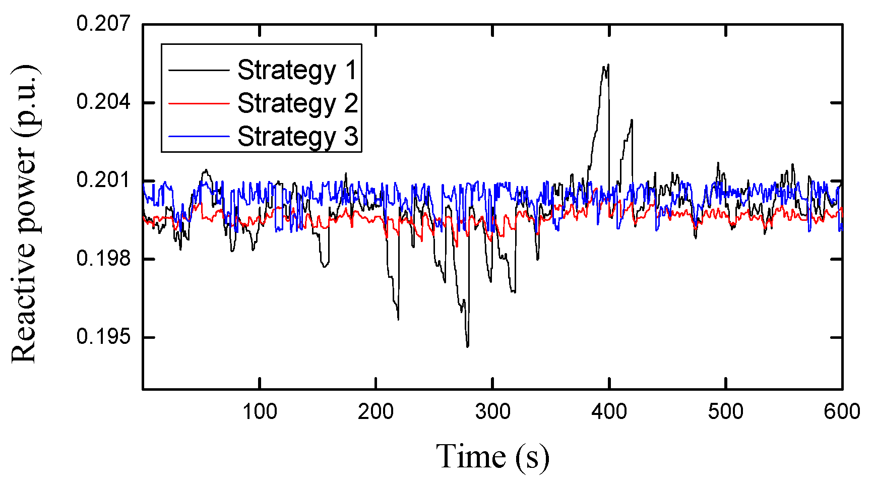
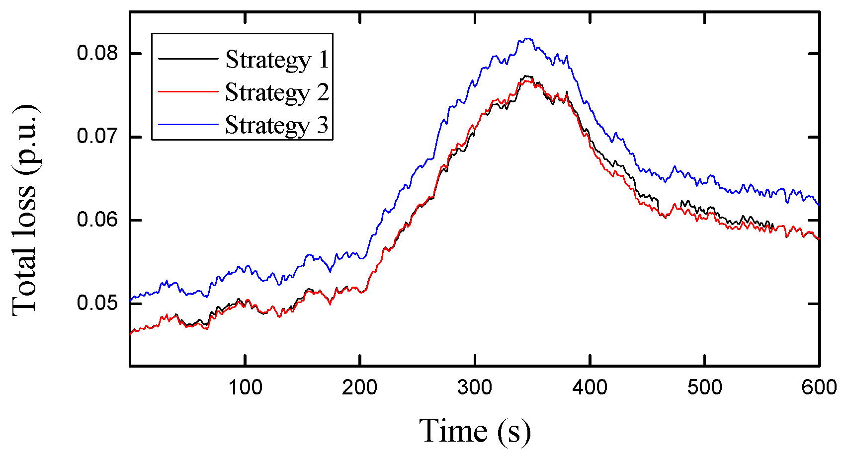
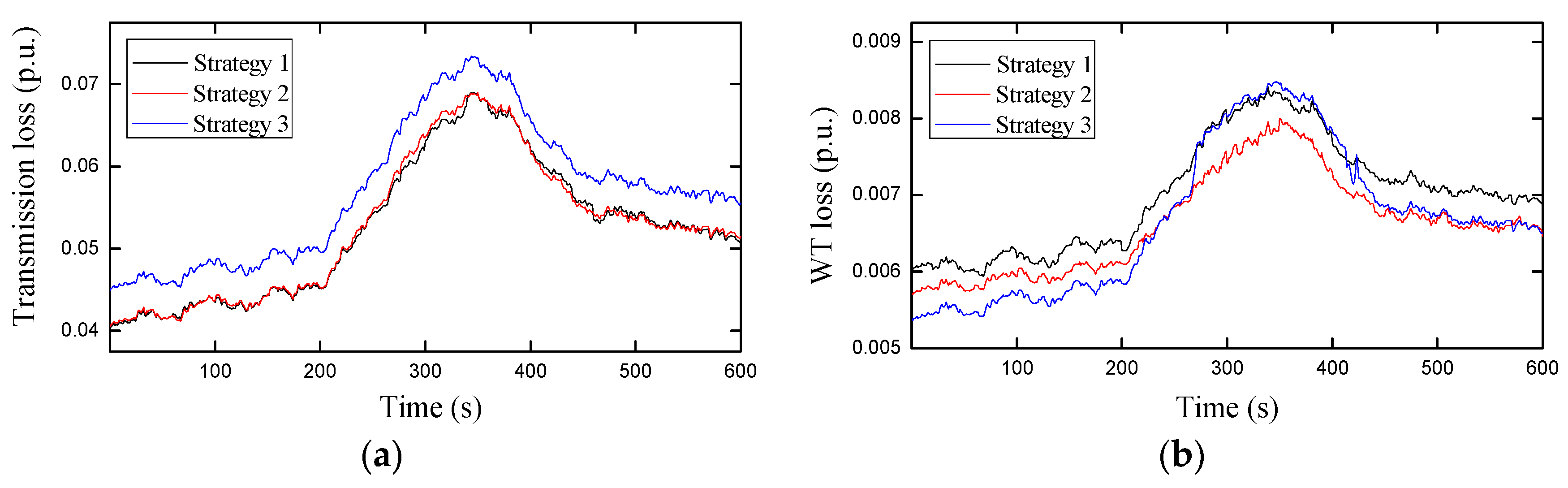
4.1. Case 1 Reactive Power of WF Remains Constant

In this case, it is assumed that the WF needs to output 0.2 p.u. reactive power.

The total reactive power output of the WF with different control strategies is shown in Figure 8. The WF using Strategy 1 cannot track the reactive power dispatching requirement of the power grid at 220 s, 280 s, and 400 s, etc. When using Strategy 2 and Strategy 3, the total reactive power output of the WF can meet the reactive power requirement of the power grid.

The total active power output of the WF with different control strategies is shown in Figure 9. It can be seen that the total active power output with Strategy 1 is always similar to that with Strategy 2, while both are about 0.05 p.u. larger than that with Strategy 3.

The total losses of the WF with different control strategies are shown in Figure 10. It can be seen that the total losses of the WF varies with wind power. When using Strategy 1 and Strategy 2, the total losses of the WF are similar, while using Strategy 3, the total losses of the WF are about 0.005 p.u. larger than those of Strategies 1 and 2. That proves the result of Figure 9.

The losses components are shown in Figure 11. As can be seen from Figure 11a, when using Strategy 1 and Strategy 2, the transmission losses of the WF are similar. Moreover, they are smaller than those using Strategy 3. Figure 11b shows that when using Strategy 1, the losses of WTs are bigger than those using Strategy 2. The losses of WTs using Strategy 2 are bigger than those using Strategy 3 from 0 s to 230 s. However, the losses using the two strategies are similar during 230 s and 280 s. The losses of the WTs using Strategy 2 are less than those using Strategy 3 from 280 s to 420 s. However, the two curves become similar again after 420 s.

The above simulation results show that when the wind power is small, compared with strategy 3, the transmission losses with Strategy 1 and Strategy 2 are lower, but their WTs’ losses are larger. This means that Strategy 1 and Strategy 2 minimize the total losses of the WF by reducing the transmission losses, but increase the losses of the WTs. When the wind power is large, the losses of the WTs increase. At this time, Strategy 1 and Strategy 2 can reduce both transmission losses and WTs’ losses to minimize the total losses of the WF.

In order to find what causes this phenomenon, we show the main losses in WTs with strategies 1, 2, and 3. Figure 12 shows the converter losses and copper losses. In Figure 12a, the losses of the converter with Strategy 1 are greater than those with Strategy 2. The converter losses with Strategy 2 are greater than those with Strategy 3 when the wind power is small (such as from 0 s to 280 s and from 420 s to 600 s, etc.). However, the opposite is true when the wind power is large (such as from 280 s to 420 s), as shown in Figure 12b, and the copper losses with Strategy 1 are greater than those with Strategy 2. The copper losses with Strategy 2 are greater during 0 s and 230 s, similar during 230 s and 250 s, and less after 250 s than those with Strategy 3.

Compared with using strategy 3, the total losses of the WF using Strategy 1 and Strategy 2 are smaller, and the total active power output is larger. Strategy 1 cannot completely track the reactive power dispatching requirement of the power grid. While, Strategy 2 and Strategy 3 can do that. Therefore, when the wind power changes and the reactive power references of the WF are constant, the performance with the proposed control strategy is better than that with the two other control strategies.

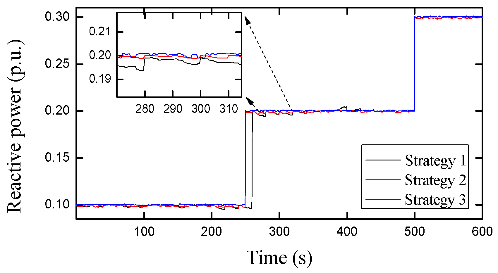
4.2. Case 2 Reactive Power of WF Remains Change

In this case, it is assumed that the reactive power references of the WF are mutative, as is shown in Figure 13. From 0 s to 250 s, the reactive power reference value is 0.1 p.u., and 0.2 p.u. from 250 s to 500 s, after that it changes to 0.3 p.u.

The total reactive power output of the WF with different control strategies are shown in Figure 14. As in case 1, the WF using Strategy 1 cannot track the reactive power dispatching requirement of the power grid when the wind power changes to become large, the error is about 0.01 p.u. The difference is that Strategy 1 also cannot do that between 250 s and 260 s because the reactive power reference value changes to 0.2 p.u. at 250 s. However, Strategy 1 can follow that change at 260 s because its running period is 20 s. Using Strategy 2 and Strategy 3, the WF can track the reactive power dispatching instruction of the power grid within the accuracy requirements.

The total active power output of the WF with different control strategies are shown in Figure 15. The active power output with Strategy 1 and Strategy 2 are similar and about 0.01 p.u. larger than those with Strategy 3. This is the same as the result of case 1.

The total losses of the WF with different strategies are shown in Figure 16. It can be seen that the total losses of the WF increase with the increase in wind power or reactive power reference value. The curve of Strategy 1 is similar to that of Strategy 2. Moreover, the total WF losses with these strategies are lower than those with Strategy 3.

Figure 17 shows the transmission losses and WTs’ losses. In Figure 17a, the transmission losses with Strategy 1 and Strategy 2 are less than those with Strategy 3. Figure 17b shows that when both the wind power and WF reactive power reference values are small, the losses of the WTs with Strategy 1 and Strategy 2 are larger than those with Strategy 3. In other cases, the losses of the WTs with Strategy 3 are no longer the smallest. This means that Strategy 1 and Strategy 2 reduce the total losses of the WF mainly by reducing the transmission losses when both the wind power and the WF reactive power reference value are small. However, they can reduce all WTs’ losses in other cases.

Figure 18 shows the converter losses and copper losses. The converter losses of the three strategies are similar to Case 1 before 250 s. The converter losses with Strategy 1 are larger than those with Strategy 3. Meanwhile, the converter losses with Strategy 3 are larger than those with Strategy 2 from 420 s to 500 s. During this time, the wind power is small, but the reactive power reference value of WF is large. However, the converter losses with Strategy 1 and Strategy 2 are less than those with Strategy 3 when both the WF reactive power reference value and wind power are large (such as from 280 s to 420 s, and from 500 s to 600 s). In Figure 18b, the trends of copper losses are similar to that in Figure 18a.

The above simulation results show that when both the wind power and the WF reactive power reference value are small, Strategy 1 and Strategy 2 can reduce the total losses. As a result, this will cause both the converter losses and the copper losses of the WTs increasing. On the contrary, they can reduce these two losses simultaneously.

When the reactive power references of the WF are mutative, the total active power output with Strategy 1 and Strategy 2 are greater than those with Strategy 3. Strategy 1 cannot completely track the reactive power dispatching instruction of the power grid but Strategy 2 and Strategy 3 can do that. Therefore, in this case, the performance with the proposed control strategy is better than that with the two other control strategies.

5. Conclusions

When the traditional control strategies are used for large WFs, the number of variables optimized is large and the control period must be long, which means the optimization effect deteriorates. To improve this, a grouped optimization control strategy is proposed to optimize the distribution of reactive power among the WTs rapidly. It distributes the reactive power requirements in each group by a proportional control strategy and uses the PSO algorithm to optimize the distribution of reactive power among groups. That reduces the variables for optimization and shortens the control period. Therefore, compared with traditional control strategies, the proposed control strategy increases the total active power output of the WF and enables the WF to track the reactive power dispatching instruction of the power grid. The simulation results verify the strategies advantages.

References

1. Toulabi, M.; Bahrami, S.; Ranjbar, A.M. Application of Edge Theorem for Robust Stability Analysis of a Power System with Participating Wind Power Plants in Automatic Generation Control Task. IET Renew. Power Gener. 2017, 11, 1049–1057. [Google Scholar] [CrossRef]
2. Lin, Y.; Yang, M.; Wan, C.; Wang, J.; Song, Y. A Multi-Model Combination Approach for Probabilistic Wind Power Forecasting. IEEE Trans. Sustain. Energy 2019, 10, 226–237. [Google Scholar] [CrossRef]
3. Mahzouni-Sani, M.; Hamidi, A.; Nazarpour, D.; Golshannavaz, S. Multi-objective Linearised Optimal Reactive Power Dispatch of wind-integrated Transmission Networks. IET Gener. Transm. Distrib. 2019, 13, 2686–2696. [Google Scholar] [CrossRef]
4. Shao, H.; Cai, X.; Li, Z.; Zhou, D.; Sun, S.; Guo, L.; Cao, Y.; Rao, F. Stability Enhancement and Direct Speed Control of DFIG Inertia Emulation Control Strategy. IEEE Access 2019, 7, 120089–120105. [Google Scholar] [CrossRef]
5. Wu, X.; Guan, Y.; Yang, X.; Ning, W.; Wang, M. Low-cost Control Strategy Based on Reactive Power Regulation of DFIG-based Wind Farm for SSO Suppression. IET Renew. Power Gener. 2019, 13, 33–39. [Google Scholar] [CrossRef]
6. Xi, X.; Geng, H.; Yang, G. Torsional Oscillation Damping Control for DFIG-Based Wind Farm Participating in Power System Frequency Regulation. In Proceedings of the 2016 IEEE Industry Applications Society Annual Meeting, Portland, OR, USA, 2–6 October 2016; Volume 4, pp. 1–5. [Google Scholar] [CrossRef]
7. Shi, K.; Yin, X.; Jiang, L.; Liu, Y.; Hu, Y.; Wen, H.; Xin, Y. Perturbation Estimation Based Nonlinear Adaptive Power Decoupling Control for DFIG Wind Turbine. IEEE Trans. Power Electron. 2019, 35, 319–333. [Google Scholar] [CrossRef]
8. Tang, W.; Hu, J.; Chang, Y.; Liu, F. Modeling of DFIG-Based Wind Turbine for Power System Transient Response Analysis in Rotor Speed Control Timescale. IEEE Trans. Power Syst. 2018, 33, 6795–6805. [Google Scholar] [CrossRef]
9. Peng, L.; Yuting, W.; Haosheng, H.; Xiangping, K.; Yubo, Y. A Coodinated Voltage Control Scheme for Power System with Large-Scale Wind Power Integration. In Proceedings of the International Conference on Renewable Power Generation (RPG 2015), Beijing, China, 17–18 October 2015; pp. 1–5. [Google Scholar]
10. Lee, K.; Ha, J.-I. Minimum Copper Loss Control of Doubly-Fed Induction Generator for Wind Turbines. In Proceedings of the 2014 IEEE Symposium on Power Electronics and Machines for Wind and Water Applications, Milwaukee, WI, USA, 24–26 July 2014; pp. 1–6. [Google Scholar] [CrossRef]
11. Kanna, B.; Singh, S.N. Towards Reactive Power Dispatch Within a WF Using Hybrid PSO. Int. J. Elect. Power Energy Syst. 2015, 69, 232–240. [Google Scholar] [CrossRef]
12. Zhang, X.; Wang, X.; Qi, X. Reactive Power Optimization for Distribution System with Distributed Generations Based on AHSPSO Algorithm. In Proceedings of the 2016 China International Conference on Electricity Distribution (CICED), Institute of Electrical and Electronics Engineers (IEEE), Xi’an, China, 10–13 August 2016; pp. 1–4. [Google Scholar] [CrossRef]
13. Zhang, B.; Hu, W.; Hou, P.; Chen, Z. Reactive Power Dispatch for Loss Minimization of a Doubly Fed Induction Generator Based Wind Farm. In Proceedings of the 2014 17th International Conference on Electrical Machines and Systems (ICEMS) IEEE, Hangzhou, China, 22–25 October 2014; pp. 1373–1378. [Google Scholar] [CrossRef]
14. Guo, Y.; Gao, H.; Wu, Q.; Zhao, H.; Østergaard, J. Coordinated Voltage Control Scheme for VSC-HVDC Connected Wind Power Plants. IET Renew. Power Gener. 2018, 12, 198–206. [Google Scholar] [CrossRef] [Green Version]
15. Liu, J.H.; Cheng, J.-S. Online Voltage Security Enhancement Using Voltage Sensitivity-Based Coherent Reactive Power Control in Multi-Area Wind Power Generation Systems. IEEE Trans. Power Syst. 2021, 36, 2729–2732. [Google Scholar] [CrossRef]
16. Yao, Q.; Hu, Y.; Chen, Z. Active Power Dispatch Strategy of the Wind Farm Based on Improved Multi-Agent Consistency Algo-Rithm. IET Renew. Power Gener. 2019, 9, 2693–2704. [Google Scholar] [CrossRef]
17. Yang, J.; Zheng, S.; Song, D.; Su, M.; Yang, X.; Joo, Y.H. Comprehensive Optimization for Fatigue Loads of Wind Turbines in Complex-Terrain Wind Farms. IEEE Trans. Sustain. Energy 2021, 12, 909–919. [Google Scholar] [CrossRef]
18. Guo, Y.; Gao, H.; Xing, H.; Wu, Q.; Lin, Z. Decentralized Coordinated Voltage Control for VSC-HVDC Connected Wind Farms Based on ADMM. IEEE Trans. Sustain. Energy 2019, 10, 800–810. [Google Scholar] [CrossRef] [Green Version]
19. Huang, S.; Wu, Q.; Bao, W.; Hatziargyriou, N.D.; Ding, L.; Rong, F. Hierarchical Optimal Control for Synthetic Inertial Response of Wind Farm Based on Alter-Nating Direction Method of Multipliers. IEEE Trans. Sustain. Energy 2021, 1, 25–35. [Google Scholar] [CrossRef]
20. Ye, L.; Zhang, C.; Tang, Y.; Zhong, W.; Zhao, Y.; Lu, P.; Zhai, B.; Lan, H.; Li, Z. Hierarchical Model Predictive Control Strategy Based on Dynamic Active Power Dispatch for Wind Power Cluster Integration. In Proceedings of the 2020 IEEE Power & Energy Society General Meeting (PESGM), Online Event, 3–6 August 2020; Volume 6, p. 1. [Google Scholar] [CrossRef]
21. Rong, F.; Ning, X.; Zhai, Y.; Zhou, S.; Huang, Y.; Yang, G. Research on Grouped Optimization Control Strategy for Large DFIG Based Wind Farm. In Proceedings of the 2020 8th International Conference on Power Electronics Systems and Applications (PESA), Institute of Electrical and Electronics Engineers (IEEE), Hong Kong, China, 7–10 December 2020; pp. 1–5. [Google Scholar] [CrossRef]
22. Zhang, B.; Hu, W.; Hou, P.; Tan, J.; Soltani, M.; Chen, Z. Review of Reactive Power Dispatch Strategies for Loss Minimization in a DFIG-Based Wind Farm. Energies 2017, 10, 856. [Google Scholar] [CrossRef] [Green Version]
23. Zhang, B.; Hou, P.; Hu, W.; Soltani, M.; Chen, C.; Chen, Z. A Reactive Power Dispatch Strategy with Loss Minimization for a DFIG-Based Wind Farm. IEEE Trans. Sustain. Energy 2016, 7, 914–923. [Google Scholar] [CrossRef]
24. Ouyang, J.; Tang, T.; Yao, J.; Li, M. Active Voltage Control for DFIG-Based Wind Farm Integrated Power System by Coordinating Active and Reactive Powers Under Wind Speed Variations. IEEE Trans. Energy Convers. 2019, 34, 1504–1511. [Google Scholar] [CrossRef]
Figure 1. Basic configuration of DFIG.
Energies 14 04848 g001
Figure 2. Cable model of transmission network.
Energies 14 04848 g002
Figure 3. Typical configuration of WF.
Energies 14 04848 g003
Figure 4. Grouped power flow model of DFIG WF.
Energies 14 04848 g004
Figure 5. Power flow of group m. Where P 0 m + jQ 0 m is the power flowing away from group m − 1. In group m, P i m + jQ i m is the power flowing away from node i to node i + 1, and P wt , i m + jQ wt , i m is the complex power output by the ith WT, where i = 1, 2,..., Nm.
Energies 14 04848 g005
Figure 6. The diagram of grouped optimization control strategy for DFIG WF.
Energies 14 04848 g006
Figure 7. Wind power for WF.
Energies 14 04848 g007
Figure 8. Total reactive power output of WF with different control strategies.
Energies 14 04848 g008
Figure 9. Total active power output of WF with different control strategies.
Energies 14 04848 g009
Figure 10. Total losses of WF with different control strategies.
Energies 14 04848 g010
Figure 11. The losses components of WF with different control strategies: (a) Transmission losses of WF; (b) WTs’ losses of WF.
Energies 14 04848 g011
Figure 12. The main losses components of WTs with different control strategies: (a) Converter losses of WTs; (b) Copper losses of WTs.
Energies 14 04848 g012
Figure 13. Total reactive power reference value of WF.
Energies 14 04848 g013
Figure 14. Total reactive power output of WF with different control strategies.
Energies 14 04848 g014
Figure 15. Total active power output of WF with different control strategies.
Energies 14 04848 g015
Figure 16. Total losses of WF with different strategies.
Energies 14 04848 g016
Figure 17. The losses components of WF with different control strategies: (a) Transmission losses of WF; (b) WTs’ losses of WF.
Energies 14 04848 g017
Figure 18. The main losses components of WTs with different control strategies: (a) Converter losses of WTs; (b) Copper losses of WTs.
Energies 14 04848 g018