Electric Field and Temperature Simulations of High-Voltage Direct Current Cables Considering the Soil Environment ^†

Abstract

For long distance electric power transport, high-voltage direct current (HVDC) cable systems are a commonly used solution. Space charges accumulate in the HVDC cable insulations due to the applied voltage and the nonlinear electric conductivity of the insulation material. The resulting electric field depends on the material parameters of the surrounding soil environment that may differ locally and have an influence on the temperature distribution in the cable and the environment. To use the radial symmetry of the cable geometry, typical electric field simulations neglect the influence of the surrounding soil, due to different dimensions of the cable and the environment and the resulting high computational effort. Here, the environment and its effect on the resulting electric field is considered and the assumption of a possible radial symmetric temperature within the insulation is analyzed. To reduce the computation time, weakly coupled simulations are performed to compute the temperature and the electric field inside the cable insulation, neglecting insulation losses. The results of a weakly coupled simulation are compared against those of a full transient simulation, considering the insulation losses for two common cable insulations with different maximum operation temperatures. Due to the buried depth of HV cables, an approximately radial symmetric temperature distribution within the insulation is obtained for a single cable and cable pairs when, considering a metallic sheath. Furthermore, the simulations show a temperature increase of the earth–air interface above the buried cable that needs to be considered when computing the cable conductor temperature, using the IEC standards.

1. Introduction

In comparison to high-voltage alternating current (HVAC) cables, high-voltage direct current (HVDC) cables are commonly used for long distance transmission of high electric power. For the connection of industrial centers to offshore wind parks or the connection of different countries across seas, e.g., in Europe, HVDC cables are used more often [1].

Differences between the electric field distributions within AC and DC cables result from the constant applied voltage and the nonlinear electric conductivity κ of the insulation. The electric field within AC cables is determined by the geometry and the permittivity ε = ε₀ε_r, with the dielectric constant ε₀ = 8.854 × 10⁻¹² As/(Vm) and the relative permittivity of the insulating material ε_r. The electric field in DC cables is defined by the nonlinear electric conductivity that mostly depends on the temperature T and the electric field stress $\overrightarrow{E}$ = −grad(φ), where φ is the scalar electric potential. As a result, space charges accumulate and yield a slowly time varying electric field. Due to the low electric conductivity, a stationary electric field is obtained at a time t ≈ 10τ after the cable is energized, with the time constant τ = ε/κ [2,3,4].

Common insulation materials of power cables are paper-based insulations, like mass-impregnated paper (MI), or polymeric materials, e.g., cross-linked polyethylene (XLPE). The materials have a maximum operation temperature of 55 °C (MI) and of 90 °C (XLPE), respectively. Power losses, due to the current inside the conductor and the leakage current in the insulation generate heat and result in a temperature drop in the cable materials and the environment. Depending on the material parameters of the ground environment, including soil and cable channel constructions, both the electric field and the temperature distributions inside the insulation and the environment vary and may show no radial symmetry [2].

To determine the time dependent electro-quasistatic (EQS) field inside a cable insulation, numerical simulations are less expensive and time consuming in comparison to measurements. Considering insulation losses and the nonlinear electric conductivity, a coupled electro-thermal field problem needs to be solved. Due to different dimensions of the environment and the cable itself, high computation times of coupled field simulations are needed.

Transient electro-quasistatic field simulations of different HV components are widely used in literature (e.g., see [5,6,7]). An additional consideration of the temperature distribution in the computational models is seen in [2,3,8,9]. In [2,9], the temperature distribution is computed with predetermined conductor and sheath temperatures and the environment around the cable is neglected. In [3,8], the temperature is computed by the generated heat in the conductor/insulation and the dissipated heat at the sheath. In [2,3,8,9], the environment is not considered to reduce the computational effort and the temperature distribution within the insulation is assumed to be radial symmetric. Furthermore, only a single cable is computed.

Here, the electric and the thermal field of single cables and cable pairs are simulated in weakly coupled simulations and the obtained results are compared against full transient simulations to analyze the applicability of an assumption of a radial symmetric temperature within the insulation. For the weak coupling, the insulation losses are neglected. As analyzed in this article, the insulation losses show a minor influence on the total temperature distribution, compared to the generated heat in the conductor. The surrounding environment is characterized utilizing different thermal conductivities [10]. Furthermore, the simulation results are compared against analytic temperature formulations used for the design of power cables.

The paper is organized as follows: after this introduction, Section 2 introduces the transient and coupled electro-thermal field problem, where a corresponding dimensionally reduced model is presented in Section 3. Simulation results of the temperature and the electric field are presented and discussed in Section 4. The results are summarized within the conclusions in Section 5.

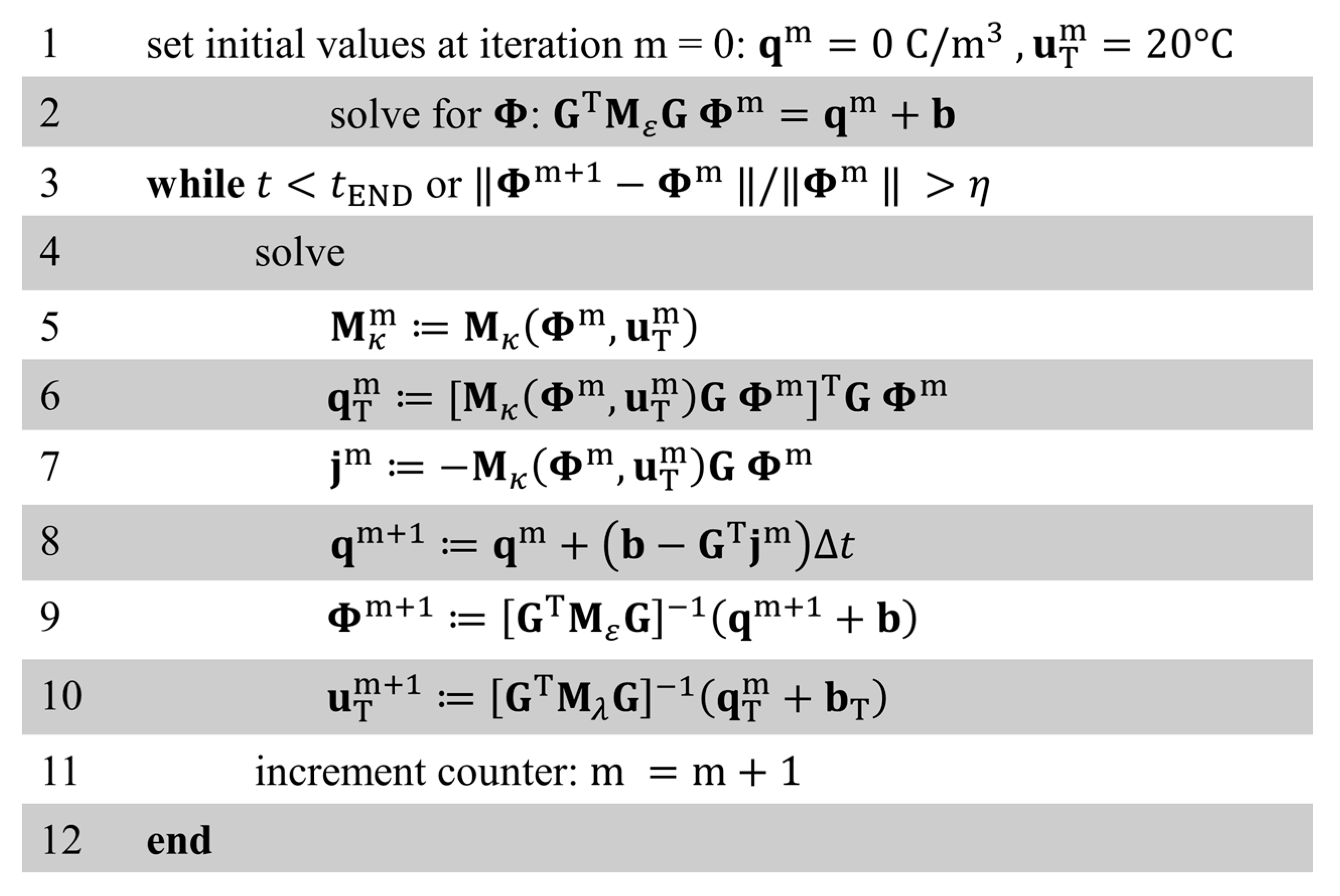
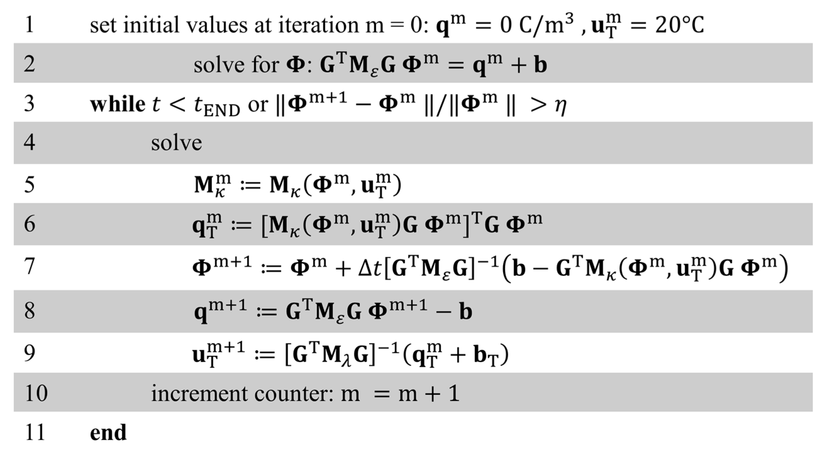
2. Numerical Computation of the Coupled Electro Thermal Field

In literature, two field formulations are introduced to compute the transient electro-quasistatic field. The “space charge oriented field formulation” e.g., found in [2] or the “scalar potential field formulation” presented e.g., in [5,6,7] are approximations of Maxwell’s equations, based on the assumption of an irrotational electric field, i.e., $\mathrm{rot}\hspace{0.17em}\overrightarrow{E}=0$. For the space charge formulation, the continuity equation, Poisson’s equation and Ohm’s law, i.e.,

$$\mathrm{div}\hspace{0.17em}\overrightarrow{J}+\frac{\partial \rho }{\partial t}=0,$$

(1)

$$\mathrm{div}\left({\epsilon }_0{\epsilon }_{\mathbf{r}}\hspace{0.17em}\mathrm{grad}\hspace{0.17em}\phi \right)=-\rho ,$$

(2)

$$\overrightarrow{J}=\kappa \left(T,\left|\overrightarrow{E}\right|\right)\overrightarrow{E}=-\kappa \left(T,\left|\overrightarrow{E}\right|\right)\mathrm{grad}\hspace{0.17em}\phi ,$$

(3)

are used, with the current density inside the insulation $\overrightarrow{J}$ and the space charge density ρ. Utilizing Equations (1)–(3), results for the space charge density and the electric field are computed. The scalar potential formulation is obtained by Equation (1), replacing ρ and $\overrightarrow{J}$ with Equations (2) and (3) and finally given by

$$\mathrm{div}\left(\kappa \left(\mathrm{T},\left|\overrightarrow{E}\right|\right)\mathrm{grad}\hspace{0.17em}\phi \right)+\frac{\partial }{\partial T}\mathrm{div}\left({\epsilon }_0{\epsilon }_{\mathbf{r}}\hspace{0.17em}\mathrm{grad}\hspace{0.17em}\phi \right)=0.$$

(4)

The solution of Equation (4) yields only the potential, and the corresponding space charge density is obtained in a postprocessing step, using Equation (2). Nearly identical results are obtained by utilizing both formulations; however, tests in [11] showed that the scalar potential field formulation has better stability characteristics.

Due to different thermal and electric time constants and a maximum charge density occurring at a stationary temperature, only the stationary configuration is used to estimate a worst-case scenario with respect to the temperature distribution [3,4]. With insulation losses Q = κ(T,|$\overrightarrow{E}$|)|$\overrightarrow{E}$|², the stationary heat conduction equation is given by

$$\mathrm{div}(\lambda \hspace{0.17em}\mathrm{grad}\hspace{0.17em}T)=-Q,$$

(5)

with the material’s thermal conductivity λ and the temperature T.

Using e.g., the finite element method (FEM) or the finite integration technique (FIT), Equations (1)–(3) are spatially discretized with given boundary conditions and result in a nonlinearly coupled system of equations

$${\mathbf{G}}^{\mathrm{T}}\mathbf{j}+\frac{d}{d\mathrm{T}}\mathbf{q}=\mathbf{b},$$

(6)

$${\mathbf{G}}^{\mathrm{T}}{\mathbf{M}}_{\epsilon }\mathbf{G}\mathsf{\Phi }=\mathbf{q}+\mathbf{b},$$

(7)

$$\mathbf{j}=-{\mathbf{M}}_{\kappa }(\mathsf{\Phi },{\mathbf{u}}_{\mathrm{T}})\mathbf{G}\mathsf{\Phi },$$

(8)

with the vector of nodal scalar potentials Φ, the vector of nodal temperatures ${\mathbf{u}}_{\mathrm{T}}$, the vector of electric dual cell charges q, the vector of current densities j, the vector b containing the boundary conditions for the electric problem, the discrete divergence matrix G^T, the conductivity matrix M_κ, the gradient matrix G and the permittivity matrix M_ε [10]. The discretization of the formulation in Equation (4) yields

$${\mathbf{G}}^{\mathrm{T}}{\mathbf{M}}_{\kappa }{(\mathsf{\Phi },\mathbf{u}}_{\mathrm{T}})\mathbf{G}\mathsf{\Phi }+\frac{d}{d\mathrm{T}}{\mathbf{G}}^{\mathrm{T}}{\mathbf{M}}_{\epsilon }\mathbf{G}\mathsf{\Phi }=\mathbf{b},$$

(9)

showing that Equations (6)–(8) are mathematically equivalent to Equation (9) [10,11].

Applying e.g., the explicit Euler time integration method to the system of ordinary differential Equation (9), the vector of scalar potentials Φ^m+1 = Φ(t^m+1) in the discrete time step m + 1 is computed by

$${\mathsf{\Phi }}^{\mathrm{m}+1}={\mathsf{\Phi }}^{\mathrm{m}}+\Delta t{\left[{\mathbf{G}}^{\mathrm{T}}{\mathbf{M}}_{\epsilon }\mathbf{G}\right]}^{-1}\left\{\mathbf{b}-{\mathbf{G}}^{\mathrm{T}}{\mathbf{M}}_{\kappa }{(\mathsf{\Phi }}^{\mathrm{m}},{\mathbf{u}}_{\mathrm{T}}{}^{\mathrm{m}}{)\mathbf{G}\mathsf{\Phi }}^{\mathrm{m}}\right\},$$

(10)

with the time step size ∆t that needs not to exceed the time step ∆t_CFL, defined by the Courant–Friedrich–Levy (CFL) criterion, for stability reasons [12]. The time step involves the solution of a linear algebraic system of equations with a constant matrix G^TM_εG of electrostatics and renders the Euler method a semi-explicit scheme and adds it to the computational load. The vector of time independent nodal temperature is

$${\mathbf{u}}_{\mathrm{T}}{}^{\mathrm{m}}={\mathbf{u}}_{\mathrm{T}}={\left[{\mathbf{G}}^{\mathrm{T}}{\mathbf{M}}_{\lambda }\mathbf{G}\right]}^{-1}\left({\mathbf{q}}_{\mathrm{T}}+{\mathbf{b}}_{\mathrm{T}}\right),$$

(11)

with the thermal conductivity matrix M_λ and the vector b_T that contains the thermal boundary conditions. The vector of insulation losses $q_{\mathrm{T}}$ changes in time, resulting from the time varying electric field and hence, Equation (11) is updated in every time step. The time integration stops if a desired stop threshold of $\Vert {\mathsf{\Phi }}^{\mathrm{m}+1}-{\mathsf{\Phi }}^{\mathrm{m}}\Vert /\Vert {\mathsf{\Phi }}^{\mathrm{m}}\Vert <\eta$, with η $\ll$ 1 or a predefined time t = t_END is obtained. Possible pseudo codes to solve the space charge formulation in Equations (6)–(8) and the scalar potential formulation in Equation (9) are shown in Figure 1 and Figure 2. To solve the electric and thermal problem, an in-house implementation, utilizing the software Free FEM++ is applied [13].

3. Geometric Model Reduction and the Electro-Thermal Coupling

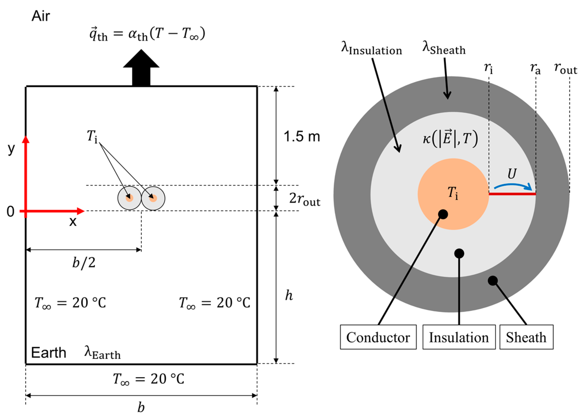
3.1. Single Cable

For the transient reference simulation including insulation losses, the two-dimensional geometry of a HVDC cable positioned in soil is depicted in Figure 3a. A sketch of the cable model geometry is shown on the right side in the same figure. The HVDC cable model is surrounded by earth and air regions, where the air region is considered with a convective heat transfer at the earth–air interface, modeling a buried underground cable [14]. The cable consists of a conductor, insulation and sheath. Additional layers, which are relatively thin for the electrical computation or less important for the thermal computation, in comparison to insulation and sheath, are neglected [8,15,16]. The insulation is either MI or XLPE. The XLPE insulation consists of two semiconducting layers, where charges may be blocked. A metallic cable sheath is neglected in the simulations due to a much higher thermal conductivity in comparison to the thermal conductivity of the insulation, sheath or earth, which results in a negligible influence on the temperature distribution.

Within the weakly coupled simulations, insulation losses are neglected, and the electric field is computed in two steps. Within the first step, the two-dimensional geometry of the cable and its environment is used for the thermal simulation. In step two, the temperature and the electric field inside the cable geometry are assumed to be radial symmetric. With temperature values at r = r_i and r = r_a and assuming a constant thermal conductivity, the stationary temperature is given by

$$T(r)=T_{\mathbf{i}}+\frac{T_{\mathbf{a}}-T_{\mathbf{i}}}{\ln \left(r_{\mathbf{a}}/r_{\mathbf{i}}\right)}\ln \left(\frac{r}{r_{\mathbf{i}}}\right).$$

(12)

and the electric field is computed along the red evaluation line in Figure 3b, using the one dimensional computation of Equations (1)–(3) or (4).

The thickness of the outer sheath is 10 mm and used for cables whose conductor cross section is 1600 mm² and the operating voltage is 400–450 kV [1,17]. Depending on the applied voltage, DC cables are buried at different depths, where HVDC cables are commonly buried at a depth of 1.5 m [14].

The thermal boundary conditions correspond to an assumed ambient temperature T_∞ = 20 °C, which is the temperature located far away from the cable. The conductor temperature is set to T_i = 90 °C for XLPE and T_i = 55 °C for MI, which are the maximum operation temperatures of both insulation materials. Temperatures close or equal to the maximum operation temperature are in general not obtained during normal operation of the cable but are used as a worst case estimation to validate the method of weakly coupled simulations. The convective heat transfer is modeled with the heat current density

$${\overrightarrow{q}}_{\mathrm{th}}={\alpha }_{\mathrm{th}}\left(T_{\mathrm{Earth}-\mathrm{Air}-\mathrm{Interface}}-T_{\infty }\right),$$

(13)

depending on the temperature of the earth–air interface T_{Earth-Air-Interface}, the temperature of the environment ${\mathrm{T}}_{\infty }$ and the heat transfer coefficient α_th [18]. The heat transfer coefficient is approximately independent on the position for low wind speeds and lies between 1 W/(m²∙K) and 2 W/(m²∙K). Assuming no wind, the coefficient is slightly lower. For the following simulations, α_th = 1.5 W/(m²∙K) is assumed.

The thermal conductivity of earth is more difficult to model and is approximated by a dependency on the humidity only. The thermal conductivity attains values between 0.47 W/(m∙K) and 2.1 W/(m∙K), where the conductivity increases with its humidity [18]. The thermal conductivities of XLPE (λ_XLPE = 0.3 W/(m∙K)) and MI (λ_MI = 0.167 W/(m∙K)) are assumed to be independent of the temperature [19,20,21]. A common material for the outer sheath is polyethylene (PE) whose thermal conductivity is λ_PE = 0.3–0.4 W/(m∙K), depending on its material density [17,18]. The dimensions of the HVDC cable and the material parameters for the insulation and the sheath are summarized in

Table 1. Dimensions for the HVDC cable in Figure 3b and material parameters of the insulation and the sheath [2,17,22,23].

Parameter	XLPE	MI
ri	23.2 mm	23.3 mm
ra	42.4 mm	42.4 mm
rout	52.4 mm	52.4 mm
λ	0.3 W/(m×K)	0.167 W/(m×K)
λPE	0.3 W/(m×K)	0.3 W/(m×K)
Ti	90 °C	55 °C
T∞	20 °C	20 °C
εr	2.3	3.5

.

To determine the computational domain, the heat current density at the boundaries is set to 1% of the heat current density at r = r_out. From the solution of the heat conduction equation for a cylindrical heat source, the heat current density is ~1/r. Thus, the distance between r_out and the domain boundary is set to 100∙r_out = 5.2 m. For example, considering an MI cable and λ_Earth = 0.47 W/(m×K), the earth–air interface temperature T_{Earth-Air-Interface} = 21.8 °C using b = 10.6 m and h = 5.2 m. This value slightly increases to T_{Earth-Air-Interface} = 21.9 °C, when using b = 22.6 m and h = 11.2 m. As a consequence, low computational effort and acceptable accuracy are obtained with the constants b = 10.6 m and h = 5.2 m in Figure 3a.

Simulation results for the stationary temperature distribution in MI and XLPE insulations are seen in Figure 4 and Figure 5. Here, the insulation losses are neglected. Nearly identical results are obtained if insulation losses are considered, and the temperature and electric field intensity are updated in every time step (reference transient simulation).

A comparison between the temperature values at the sheath (r = r_out), computed by the transient fully coupled reference simulation and a simplified simulation neglecting insulation losses, show temperature differences of <0.1%. Resulting from the computation of two systems of equations and the time integration of the explicit Euler method, the transient reference simulation requires a more extensive computational time by one order of magnitude in comparison to weakly coupled simulations. Within the weakly coupled simulations, the one-dimensional computation of the electric field does not significantly increase the computation time. Here, the simulation time of the reference simulation is about 150 s and the weakly coupled simulations need about 5 s on a computer system with Intel i5-processors, with four cores, each one with 3.2 GHz. The total RAM of the computer system is 16 GByte.

The unsymmetrical temperature distribution in Figure 4 and Figure 5 may indicate different sheath temperatures at y = 0 and y = 2∙r_out. For MI and λ_Earth = 0.47 W/(m×K), the temperature difference between y = 0 and y = 2∙r_out is 0.08 °C, whereas for λ_Earth = 2.1 W/(m × K), the temperature difference is 0.03 °C. Using a XLPE insulation and λ_Earth = 0.47 W/(m × K), the temperature difference is 0.27 °C and with λ_Earth = 2.1 W/(m × K), the temperature difference is 0.08 °C. The low differences of the temperature values at r = r_out show that a radial symmetric temperature and electric field is a reasonable assumption for the interior geometry of single buried cables. Even without a metallic screen, low deviations from symmetry are seen for single cables. Such a screen acts as an isothermal surface and results in higher symmetry, which is more clearly explained in Section 3.2.

The negligible increase of the temperature due to low insulation losses in comparison to the losses of the cable’s conductor as mentioned in [24]. For an approximate comparison between the heat losses per length inside the insulation

$$\kappa (T,|\overrightarrow{E}|)|\overrightarrow{E}{|}^2\pi (r_{\mathbf{a}}{}^2-r_{\mathbf{i}}{}^2)$$

(14)

and the heat losses per length in the conductor

$$\frac{T_{\mathbf{i}}-T(r_{\mathbf{a}})}{R_{\mathrm{th},\mathrm{Insulation}}}=\frac{T_{\mathbf{i}}-T(r_{\mathbf{a}})}{\ln (r_{\mathbf{a}}/r_{\mathbf{i}})}2\pi {\lambda }_{\mathrm{MI},\mathrm{XLPE}},$$

(15)

where

$$R_{\mathrm{th},\mathrm{Insulation}}=\frac{1}{2\pi {\lambda }_{\mathrm{Insulation}}}\ln \left(\frac{r_{\mathbf{a}}}{r_{\mathbf{i}}}\right)$$

(16)

is the thermal resistance of the insulating material per length of the cable, E = U/(r_a − r_i) and T = T(r_a) + (T_i − T(r_a))/2 are used. The conductor temperatures T_i are given with 90 °C (XLPE) or 55 °C (MI) and the applied voltage is U = 450 kV.

To compute the insulation losses in Equation (14), the electric conductivity of MI is given by the empirical relation

$$\kappa \left(T,\left|\overrightarrow{E}\right|\right)={\kappa }_0\exp \left(\alpha T\right)\exp \left(\beta \left|\overrightarrow{E}\right|\right),$$

(17)

where κ₀ = 5 × 10⁻¹⁶ S/m, α = 0.088 °C⁻¹ and β = 3 × 10⁻⁸ m/V [22]. The electric conductivity of XLPE is

$$\kappa \left(T,\left|\overrightarrow{E}\right|\right)=J_0\exp \left(\frac{-E_{\mathbf{a}}}{kT}\right)\frac{\sinh \left(\gamma \left|\overrightarrow{E}\right|\right)}{\left|\overrightarrow{E}\right|},$$

(18)

where k = 1.38 × 10⁻²³ J/K is the Boltzmann constant, J₀ = 3.6782 × 10⁷ A/m², E_a = 0.98 eV and γ = 1.086 × 10⁻⁷ m/V [8,25].

The results for both insulation materials and different thermal conductivities of the earth and thus, different temperature gradients inside the insulation, are seen in

Table 2. Computed insulation losses and conductor losses for different insulation materials and thermal conductivities of the earth.

	λEarth = 0.47 W/(m × K)	λEarth = 2.1 W/(m × K)
T(ra) in XLPE	77.9 °C	61 °C
T(ra) in MI	45.4 °C	35.4 °C
T = T(ra) + (Ti − T(ra))/2in XLPE	84 °C	75.5 °C
T = T(ra) + (Ti − T(ra))/2in MI	50.2 °C	45.2 °C
E = U/(ra − ri)in XLPE	23.4 kV/mm	23.4 kV/mm
E = U/(ra − ri)in MI	23.4 kV/mm	23.4 kV/mm
(14) in XLPE	0.3 W/m (83 W/m3)	0.2 W/m (38 W/m3)
(15) in XLPE	38 W/m (22∙103 W/m3)	91 W/m (54∙103 W/m3)
(14) in MI	0.2 W/m (46 W/m3)	0.1 W/m (30 W/m3)
(15) in MI	17 W/m (10∙103 W/m3)	34 W/m (20∙103 W/m3)

. Maximum insulation losses of Q = 83 W/m³ are computed for XLPE and of Q = 46 W/m³ for the MI insulation. To increase the temperature of 1 °C, average insulation losses of Q = 1100–1600 W/m³ are needed for MI and Q = 1600–2200 W/m³ are needed for XLPE. The loss intervals are valid within the range of λ_Earth = 0.47 W/(m × K) and λ_Earth = 2.1 W/(m × K) and much higher than the simulated values.

The effect of insulation losses increases if the electric conductivity increases. Using Equations (17) and (18), with an increasing electric field, the insulation losses increase, but considerable effects are only seen for field values above the breakdown strength of the material. The breakdown strength of the dielectric material increases with decreasing thickness [26]. With a thickness of typical HVDC cable insulations (10–30 mm), breakdown strength values of 50 kV/mm for MI and XLPE are found in literature [17,22,26,27]. In case of fast transients (impulse voltage) the insulation can resist fields above the breakdown strength for a short period of time. Thus, high electric conductivity values and insulation losses are given within the insulation. On the other hand, the duration time is very short, and a considerable increase in temperature is not seen. As a consequence, neglecting the insulation losses inside the cable geometry is an applicable approach to obtain the temperature in buried HVDC cables and to reduce the computational effort.

The thickness of the outer sheath is 10 mm, which is approximately half of the insulation thickness. If the outer sheath is not considered, the temperature difference within the insulation between the full geometry (with outer sheath) and the reduced geometry (without outer sheath) increases towards r_a. With an increasing humidity, the temperature difference at the outer sheath, between the full and the reduced geometry, increases to a maximum value of 2 °C in MI and 4 °C in XLPE. Thus, neglecting the outer sheath is not applicable to further reduce the geometry and the computation time.

3.2. Cable Pair Together

HVDC cables are also used in dual configurations, where the temperature of both conductors is assumed with T_i. Equal to Figure 3, the two-dimensional geometry is seen in Figure 6 and the dimensions are given in Table 1 and by b = 10.6 m and h = 5.2 m. The two cables are in direct contact, which can be considered as a worst-case scenario for the temperature. In practice, parallel cables have some mutual distance to increase their ampacity.

The simulation results of cable pairs show a non-symmetrical temperature distribution within the insulation and thus, a non-symmetrical electric field distribution. For example, the temperature distribution of a MI cable pair with λ_Earth = 2.1 W/(m × K) is depicted in Figure 7. Between both conductors (“Region A”), the temperature inside the insulation is higher compared to “Region B” but the temperature gradient is lower in “Region A”. In comparison to a single cable, the temperature at r_a is higher in both regions for each λ_Earth. As a consequence, higher temperature values are seen at the earth–air interface in comparison to a single cable (compare Figure 4 and Figure 7).

The temperature at the earth–air interface in Figure 7 is 23.9 °C for λ_Earth = 2.1 W/(m × K) and 22.3 °C for λ_Earth = 0.47 W/(m × K) and also slightly higher in comparison to 20 °C ambient temperature. Compared to a single cable (Figure 4), the temperature increases 0.5–1.4 °C due to the additional heat losses of the second cable. Using an XLPE insulation, the temperature above both cables at the earth–air interface lies between 25.1 °C (λ_Earth = 0.47 W/(m × K)) and 29.6 °C (λ_Earth = 2.1 W/(m × K)), which is an increase of 1–3 °C compared to a single cable. Buried XLPE cable pairs in close proximity show a higher influence on the environment than single cables, whereas MI single cables and cable pairs have an approximately equal influence.

Considering a metallic sheath with a thickness of 1 mm around the insulation results in an approximately radial symmetric temperature field within the insulation. Due to the high thermal conductivity of the metallic sheath (λ_Aluminum = 236 W/(m × K)) in comparison to the insulation or the outer sheath, the non-symmetry of the temperature distribution within the insulation is reduced, due to approximately constant temperature values at r = r_a. For example, Figure 8 shows the temperature distribution within “Region A” and “Region B” of the right cable in Figure 7, at y = r_out. Considering the metallic sheath, the temperature drop within the insulation is approximately equal in “Region A” and “Region B” and between the temperature drops without considering a metallic sheath. The temperature at the earth–air interface negligibly increases due to the metallic sheath. Thus, one-dimensional electric field simulations inside cable geometries are also applicable for cable pairs, if a metallic sheath is considered.

In power cable designs, the metallic screen usually consists of separate strands. With a bad thermal contact between these, the separate wires can have slightly different temperature values. Nevertheless, the symmetry of the temperature inside the insulation is not reduced due to a twist of the strands around the cable. The temperature is averaged because each strand will encounter all positions around the cable.

4. Simulation Results of the Temperature and the Electric Field

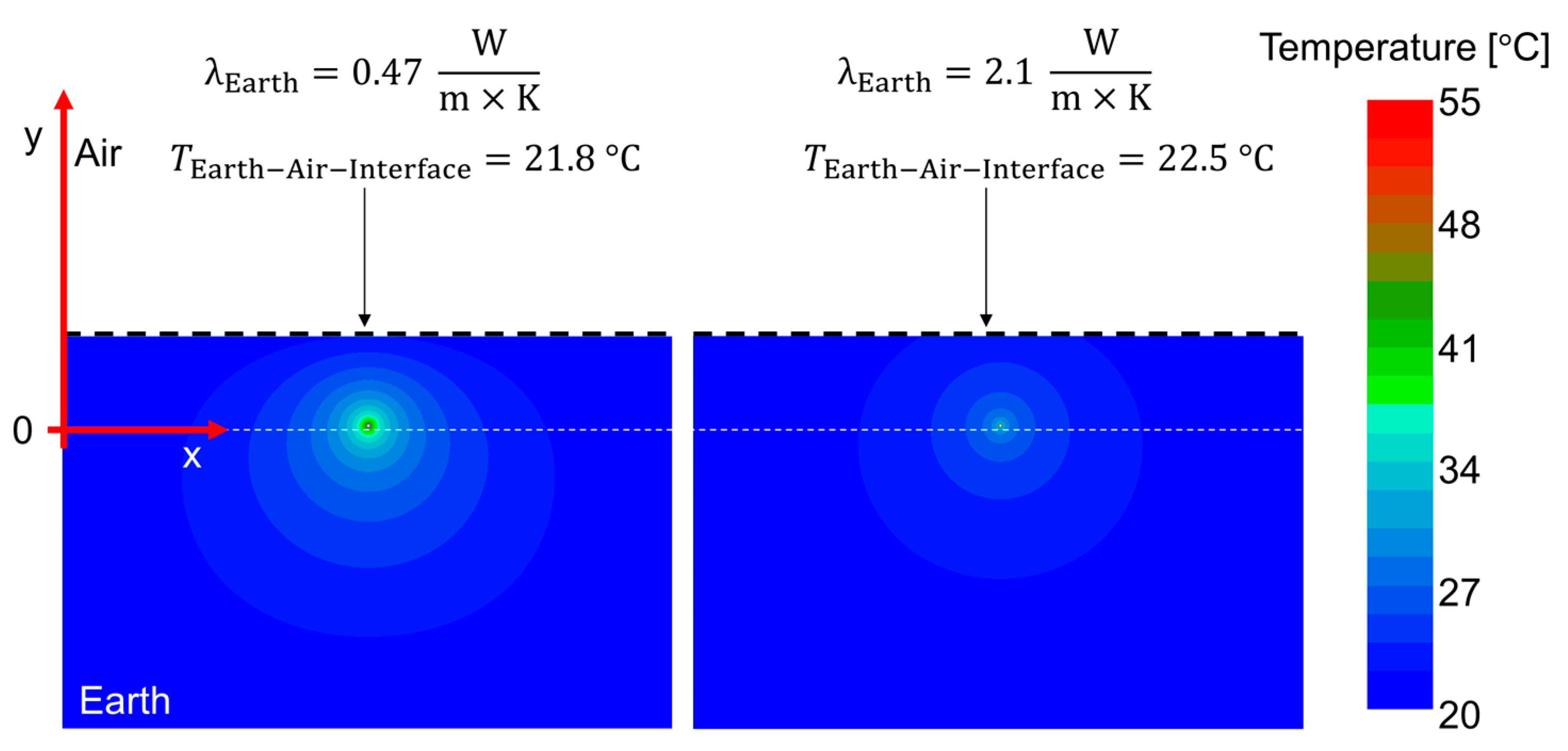
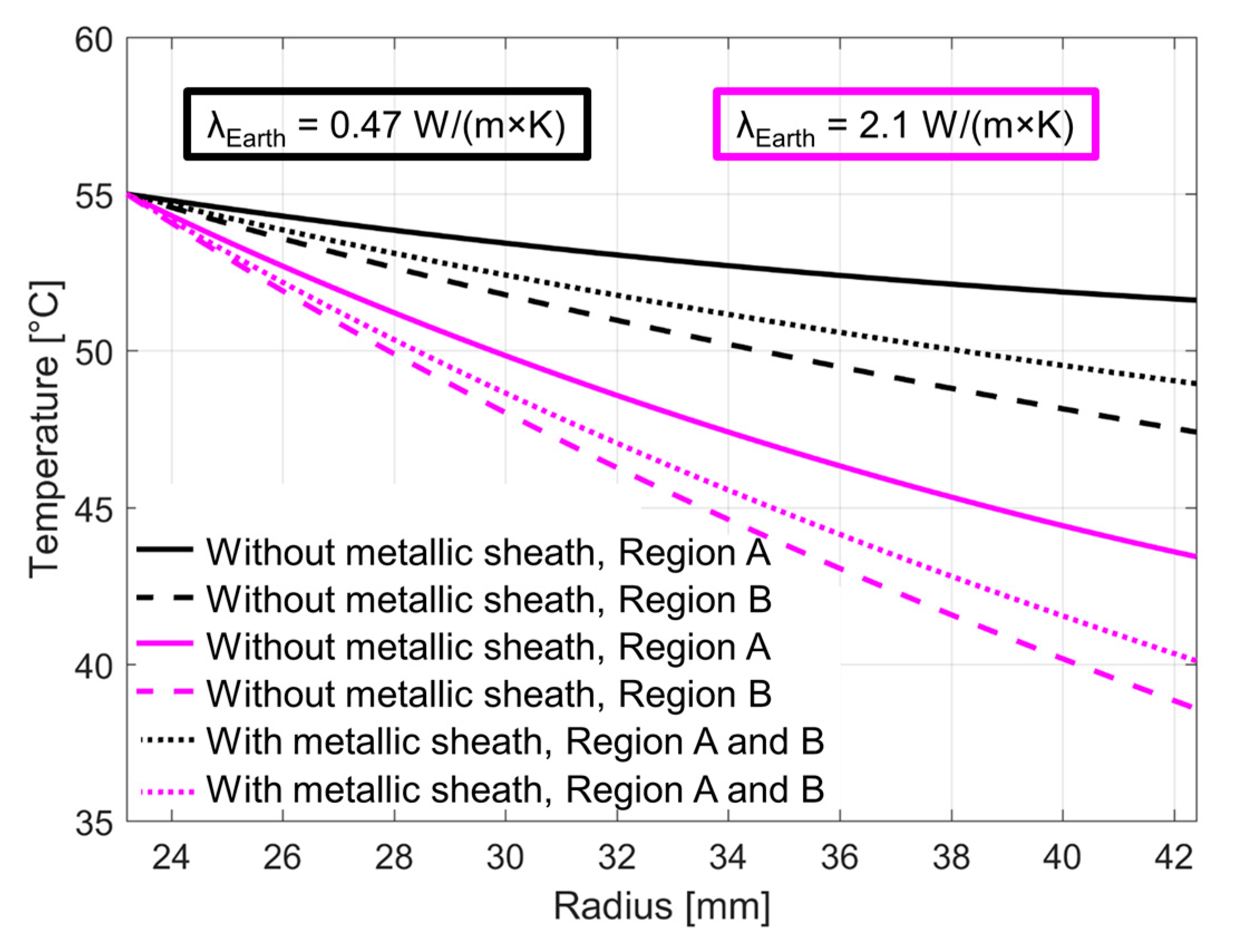
4.1. MI Cable Insulation

Humidity variations result in varying thermal conductivity and temperature profiles within the insulation and in the environment (Figure 4 and Figure 5). Considering a single MI insulation, for example, the simulated temperature distribution is seen in Figure 4. An increase in the thermal conductivity from λ_Earth = 0.47 W/(m × K) to λ_Earth = 2.1 W/(m × K) results in a temperature increase of 0.7 °C, i.e., from 21.8 °C to 22.5 °C above the cable at the earth–air interface. The mean interface temperature is about 22 °C and thus, 2 °C above the temperature of the environment T_∞ = 20 °C. With increasing λ_Earth, the temperature gradient inside the insulation also increases, as shown in Figure 9. The vertical black dotted line (r ≈ 42 mm) indicates the interface between the cable insulation and the outer sheath. Analogously to electrostatic results, the temperature gradient inside the PE material is lower, compared to MI, due to its higher thermal conductivity (see Table 1). Resulting from thermal conductivities λ_MI < λ_PE, the total temperature gradient inside the MI insulation and the PE sheath (11.5 °C–23.4 °C, for λ_Earth = 0.47 W/(m × K)–λ_Earth = 2.1 W/(m × K)) is approximately only within the MI insulation (9.6 °C–19.6 °C, for λ_Earth = 0.47 W/(m × K)–λ_Earth = 2.1 W/(m × K)), also depicted in Figure 9.

An increase of the humidity of the surrounding earth soil is also increasing its thermal conductivity. The earth around the cable is heating up less, resulting in a decreased sheath temperature (T_out) but an increased temperature drop inside the insulation. With increasing temperature gradient, the electric field is reduced in the vicinity of the conductor, but increased near the sheath, which is the so-called “effect of field inversion” [1,2]. The field inversion occurs from the accumulation of charges in the insulation. The stationary electric field is depicted in Figure 10, where the temperature distribution in Figure 9 is used. For very dry earth (λ_Earth = 0.47 W/(m × K)), the electric field stress shows a small degree of field inversion and a rather homogeneous distribution, but an inhomogeneous field distribution is seen for very wet earth (λ_Earth = 2.1 W/(m × K)). Compared to the field stress at very dry earth (λ_Earth = 0.47 W/(m × K)), the electric field exhibits a relative decrease up to 27% near the conductor and an increase up to 23% right at the sheath, depending on the humidity.

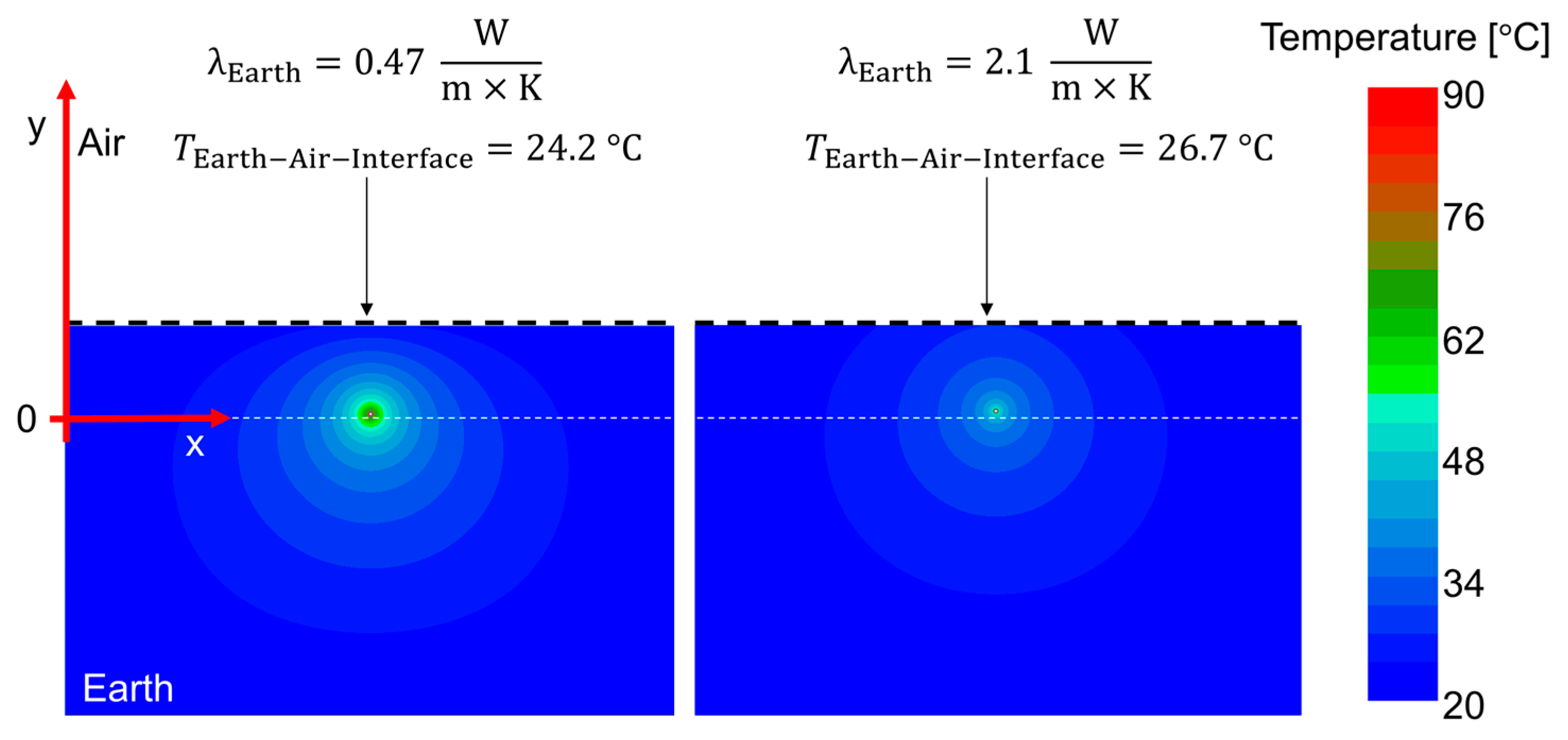
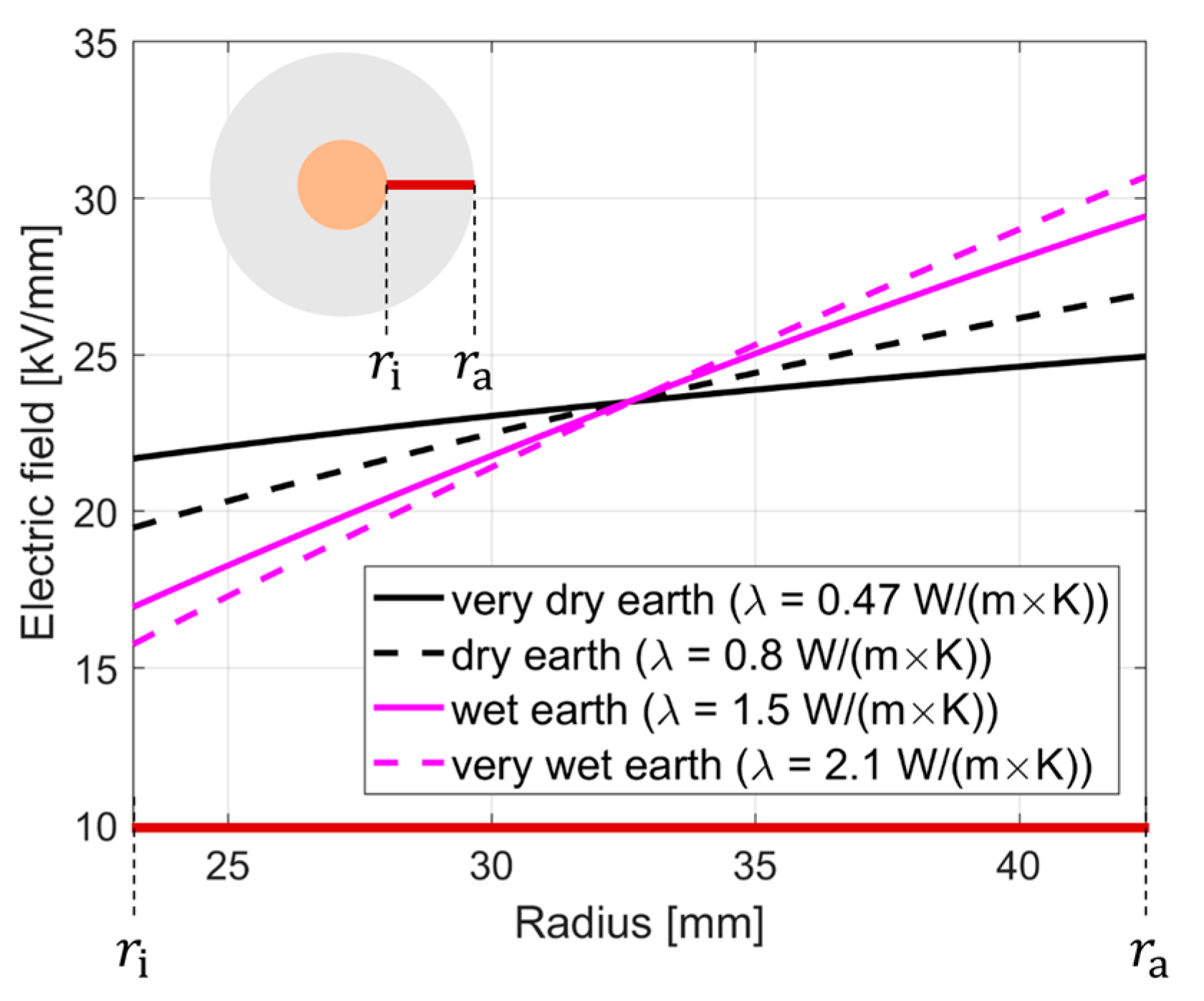
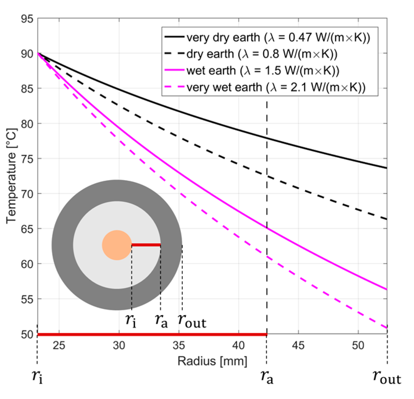
4.2. XLPE Cable Insulation

The computed temperature values within the environment of the XLPE cable are depicted in Figure 5 for λ_Earth = 0.47 W/(m × K) and λ_Earth = 2.1 W/(m × K). As a result of the higher cable core temperature the insulation can withstand, and modern XLPE underground cables have a higher effect on the environmental soil, compared to MI cables. With increasing humidity, the temperature above the cable at the earth–air interface, increases from 24.2 °C (λ_Earth = 0.47 W/(m × K)) to 26.7 °C (λ_Earth = 2.1 W/(m × K)). Thus, the mean interface temperature is about 25.5 °C and about 5 °C above the environment temperature T_∞ = 20 °C.

The computed temperature values in the insulating material and the outer sheath are depicted in Figure 11. Similar to Figure 9, the vertical black dotted line (r ≈ 42 mm) marks the insulation–sheath interface. Resulting from equal thermal conductivities λ_XLPE = λ_Sheath = 0.3 W/(m × K), the temperature drop within the XLPE and the outer sheath has a continuous distribution.

The temperature difference within the insulation lies between 12 °C at λ_Earth = 0.47 W/(m × K) and 29 °C at λ_Earth = 2.1 W/(m × K). The temperature gradient at very dry earth is nearly equal to the one in the MI cable insulation (see Figure 9), but with increasing humidity, the temperature gradient in the XLPE cable is higher in comparison to the MI cable. The higher temperature gradient results in a higher charge density and thus, in an increased electric field. Using the temperature distribution in Figure 11, the corresponding field is shown in Figure 12.

Insulation materials for DC cables are usually modified to suppress the charge accumulation and a high inversion of the field. Furthermore, high electric field and temperature values result in injection processes at both electrodes. Injected homo charges reduce the electric field and especially at the sheath, the field is lower compared to Figure 12. Thus, the electric field results in Figure 10 and Figure 12 may be considered as worst-case scenario values.

Within an annual circle, the temperature values of the environment may reach higher values than the commonly assumed average temperature of 20 °C in the summer, and also develop below this value during winter days. At high environment temperatures, the convective heat transfer is reduced and the earth soil around the cable heats up. As a consequence, the temperature gradient within the cable insulation is lower compared to the temperature gradient at T_∞ = 20 °C, which results in less stress at the sheath. Assuming environment temperature values lower than 20 °C, the convective heat transfer is increased, resulting in a higher temperature gradient and field stress within the cable insulations.

4.3. Comparison between the Temperature Calculation, Using Numerical Simulations and the Image Method

To obtain the current carrying capacity of a HVDC cable, commonly the current I is known and the temperature of the conductor T_i is computed. Within the IEC standards, to compute the conductor temperature of buried cables (IEC 60287 and IEC 60853), the image method is used assuming an earth–air interface temperature (T_{Earth-Air-Interface}) equal to the ambient temperature (T_{Earth-Air-Interface} = T_∞). This assumption might be incorrect for some configurations (see e.g., Figure 4 and Figure 5) and is discussed in this section by comparing T_{Earth-Air-Interface} and T_i against simulated values. Within the IEC standards, the conductor temperature T_i is computed by Ohms law of heat conduction, i.e.,

$$T_{\mathbf{i}}-T_{\mathrm{Earth}-\mathrm{Air}-\mathrm{Interface}}=I^2{R}_{\mathrm{Conductor}}\left(R_{\mathrm{Th},\mathrm{Insulation}}+R_{\mathrm{Th},\mathrm{Sheath}}+R_{\mathrm{Th},\mathrm{Earth}}\right),$$

(19)

with the current I and the electric resistivity per length of the conductor R_Conductor [28,29,30]. The thermal resistivity of the insulation R_{th,Insulation} is given by Equation (16) and the thermal resistivity of the sheath R_th,Sheath and the earth R_th,Earth per cable length are given by

$$R_{\mathrm{th},\mathrm{Sheath}}=\frac{1}{2\pi {\lambda }_{\mathrm{Sheath}}}\ln \left(\frac{r_{\mathrm{out}}}{r_{\mathbf{a}}}\right),$$

(20)

$$R_{\mathrm{th},\mathrm{Earth}}=\frac{{\lambda }_{\mathrm{Earth}}}{2\pi }\ln \left(\frac{h_{\mathbf{x}}}{r_{\mathrm{out}}}+\sqrt{{\left(\frac{h_{\mathbf{x}}}{r_{\mathrm{out}}}\right)}^2-1}\right),$$

(21)

where h_x = 1.5 m is the buried depth of the cable [16].

Temperature values, computed by Equation (19), are compared against reference numerical simulations. The reference temperature results are obtained by Equation (11), were the vector of insulation losses $q_{\mathrm{T}}$ is neglected within the weakly coupled simulations. Resulting from a given current I, instead of a given conductor temperature T_i, the produced heat current density has only a radial component and is given by

$$q_{\mathrm{in}}=\frac{I^2{R}_{\mathrm{Conductor}}}{2\pi r_{\mathrm{i}}}, \left[\frac{\mathrm{W}}{{\mathrm{m}}^2}\right].$$

(22)

A comparison between the conductor temperatures of a MI cable, numerically simulated and computed with Equation (19), shows similar conductor temperatures (see Figure 13) and relative differences up to 2–3% below the maximum operation temperature of T_i = 55 °C. The solid lines are the results, computed with Equation (19), and the symbols are simulation results. The conductor temperatures are computed for different environment temperatures of T_∞ = −10 °C, T_∞ = 20 °C and T_∞ = 35 °C and humidity concentrations. The computation, using Equation (19), yields slightly lower conductor temperatures. With decreasing environment temperature or increasing conductor temperature, the relative difference between both computations increases. This results from the influence of the cable core temperature on the earth–air interface temperature, as seen in Figure 14 [28]. Equal results are obtained for an equivalent XLPE cable, where higher error values (<5%), due to the higher possible conductor temperature, are evaluated.

With increasing humidity, the effect on the environment is reduced, showing temperature values T_{Earth-Air-Interface} close to T_∞ in Figure 14. On the other hand, the earth–air interface temperature T_{Earth-Air-Interface} increases with the humidity in Figure 4 and Figure 5. This results from the assumed constant conductor temperature and is also seen in Figure 13 and Figure 14. For example, in Figure 13b, the conductor temperature is 55 °C with I ≈ 1300 A (λ_Earth = 0.47 W/(m × K)) or I ≈ 1850 A (λ_Earth = 2.1 W/(m × K)). With Figure 14b, the current values correspond to T_{Earth-Air-Interface} = 21.5 °C (λ_Earth = 0.47 W/(m × K)) and T_{Earth-Air-Interface} = 22.5 °C (λ_Earth = 2.1 W/(m × K)). Thus, due to higher possible current values with increasing humidity, the temperature T_{Earth-Air-Interface} also increases, but decreases for a constant conductor current.

According to [1], the “Baltic Cable” has equal dimensions and material parameters, compared to the cable model utilized in the numerical tests. The transmitted power of the “Baltic Cable” is 600 MW, resulting in a current of I = 1333.33 A (U = 450 kV). Assuming a wet earth ground that is common in middle Europe λ_Earth ≈ 0.8 W/(m × K), the simulated earth–air interface temperature shows values of −7 °C (for T_∞ = −10 °C), 21.5 °C (for T_∞ = 20 °C) and 36.5 °C (for T_∞ = 35 °C).

Using Equation (19), the conductor temperature of buried cables is approximated with sufficient accuracy (Figure 13), but the assumption of an earth –air interface temperature equal to the environment temperature seems to be valid only for rather low conductor temperatures (current values) or deeply buried cables (Figure 14). The influence of the cable temperature is higher at low environment temperatures. Equal to results in [28], the assumption of an earth–air interface temperature equal to the environment temperature is valid for moderate temperatures. As a consequence, [29] recommends varying the environment temperature, using Equation (19), depending on the surface condition or the burial depth.

5. Conclusions

To compute the electric field within the insulation of buried HVDC cables, a coupled electro-thermal field simulation is needed, due to the nonlinear electric conductivity and the insulation losses. Furthermore, with different thermal conductivity values of the surrounded earth and air, the assumption of a radial symmetric electric field and temperature distribution is under certain configurations (e.g., no metallic sheath at cable pairs) not valid.

Due to moderate temperate values, the insulation losses showed a negligible influence on the resulting temperature distribution and weakly coupled simulations of the temperature and the electric field were applied. Corresponding to the depth at which the cable is buried, an approximately radial symmetric temperature distribution within the insulation was obtained for a single cable and cable pairs (considering a metallic sheath). Thus, to avoid long computation times, the temperature was obtained within a simulation of the two-dimensional geometry model. Having the conductor and sheath temperature, the electric field was evaluated within a one-dimensional calculation. Here, the computation time of the weakly coupled simulations are lower by one order of magnitude, in comparison to fully coupled transient simulations that also consider insulation losses and show the applicability of the research results to practical problems.

The obtained simulation results indicated a temperature distribution inside the insulation of underground HVDC cables that was shown to exhibit a dependency on the surrounding environment. With increasing humidity concentration and correspondingly increasing thermal conductivity of the environment, the temperature gradients within the insulation were also shown to increase. The resulting temperature gradients due to different humidity values showed an increasing electric field stress at the sheath.

Using the IEC standards, an earth–air interface temperature equal to the environment temperature is assumed to compute the conductor temperature. Simulation results showed that the IEC standard approximated the conductor temperature with a sufficient accuracy. Furthermore, reference simulations indicated higher temperature values at the earth–air interface by several degrees (depending on T_∞), compared to the environment temperature. An assumed environment temperature at the earth–air interface is not applicable for every circumstance and needs to vary, depending on the surface condition or the burial depth. Furthermore, other structures, like pipes or drains, as well as the dryness of the soil in the close vicinity of the cable due to their temperature have significant influence on the temperature distribution in the soil and the cable.

References

1. Mazzanti, G.; Marzinotto, M. Extruded Cables for High-Voltage Direct-Current Transmission: Advances in Research and Development; John Wiley & Sons Inc.: Hoboken, NJ, USA, 2013; pp. 49–75. ISBN 978-1-118-09666-6. [Google Scholar]
2. Jeroense, M.J.P.; Morshuis, P.H.F. Electric fields in HVDC paper-insulated cables. IEEE Trans. Dielectr. Electr. Insul. 1998, 5, 225–236. [Google Scholar] [CrossRef]
3. Jörgens, C.; Clemens, M. Thermal Breakdown in High Voltage Direct Current Cable Insulations due to Space Charges. COMPEL 2018, 37, 1689–1697. [Google Scholar] [CrossRef]
4. Steinmetz, T.; Kurz, S.; Clemens, M. Domains of Validity of Quasistatic and Quasistationary Field Approximations. COMPEL 2011, 30, 1237–1247. [Google Scholar] [CrossRef]
5. Steinmetz, T.; Helias, M.; Wimmer, G.; Fichte, L.O.; Clemens, M. Electro-Quasistatic Field Simulations Based on a Discrete Electromagnetism Formulation. IEEE Trans. Magn. 2006, 42, 755–758. [Google Scholar] [CrossRef]
6. Clemens, M.; Wilke, M.; Benderskaya, G.; DeGersem, H.; Koch, W.; Weiland, T. Transient Electro-Quasistatic Adaptive Simulation Schemes. IEEE Trans. Magn. 2004, 40, 1294–1297. [Google Scholar] [CrossRef]
7. Lupo, G.; Petrarca, C.; Egiziano, L.; Tucci, V.; Vitelli, M. Numerical Evaluation of the Field in Cable Terminations Equipped with nonlinear Grading Materials. Annual Report. In Proceedings of the Eletrical Insulation and Dielectric Phenomena (CEIDP), Atlanta, GA, USA, 25–28 October 1998; pp. 585–588. [Google Scholar] [CrossRef]
8. Liu, Y.; Zhang, S.; Cao, X.; Zhang, C.; Li, W. Simulation of Electric Field Distribution in the XLPE Insulation of a 320 kV DC Cable under Steady and Time-Varying States. IEEE Trans. Dielectr. Electr. Insul. 2018, 25, 954–964. [Google Scholar] [CrossRef]
9. Mauseth, F.; Haugdal, H. Electric Field Simulations of High Voltage DC Extruded Cable Systems. IEEE Electr. Insul. Mag. 2017, 33, 16–21. [Google Scholar] [CrossRef] [Green Version]
10. Jörgens, C.; Clemens, M. Simulation of the Electric Field in High Voltage Direct Current Cables considering the Environment. Annual Report. In Proceedings of the 10th International Conference on Computational Electromagnetics (CEM), Edinburgh, UK, 19–20 June 2019. [Google Scholar] [CrossRef]
11. Jörgens, C.; Clemens, M. Comparison of Two Electro-Quasistatic Field Formulations for the Computation of Electric Field and Space Charges in HVDC Cable Systems’. Annual Report. In Proceedings of the 22nd International Conference on the Computation of Electromagnetic Fields (COMPUMAG), Paris, France, 15–19 July 2019. [Google Scholar] [CrossRef]
12. Hairer, E.; Wanner, G. Solving Ordinary Differential Equations II: Stiff and Differential Algebraic Problems, 2nd ed.; Springer: Berlin/Heidelberg, Germany, 1996. [Google Scholar]
13. Hecht, F. New development in FreeFem++. J. Numer. Math. 2012, 20, 251–266. [Google Scholar] [CrossRef]
14. Ebert, S.; Sill, F.; Diederichs, J. Extruded XLPE DC underground-cable technology and experiences up to 525 kV—A key building block for the German “Energiewende”. In VDE High Voltage Technology 2016; Annual Report; VDE: Berlin, Germany, 2016; pp. 8–13. [Google Scholar]
15. Heinhold, L.; Stubbe, R. Kabel und Leitungen für Starkstrom; Publics MCD Verlag: Erlangen, Germany, 1999; pp. 271–295, 306–318. ISBN 3-89578-088-X. [Google Scholar]
16. Peschke, E.; Olshausen, R.v. Kabelanlagen für Hoch- und Höchstspannung; Publics MCD Verlag: Erlangen, Germany, 1998; pp. 72–77. ISBN 3-89578-057-X. [Google Scholar]
17. High Voltage Cable Systems–Cables and Accessories up to 550 kV nkt datasheet. Tech. Rep. 2012. Available online: https://www.cablejoints.co.uk/upload/NKT_Cables_Extra_High_Voltage_132kV_220kV_400kV_500kV___Brochure.pdf (accessed on 15 July 2021).
18. Spitzner, M.H. VDI Wärmeatlas, 11th ed.; Springer: Berlin/Heidelberg, Germany, 2013; pp. 196–198, 648, 686–687, 753–760. [Google Scholar] [CrossRef]
19. Qi, X.; Boggs, S.A. Thermal and Mechanical Properties of EPR and XLPE Cable Components. IEEE Electr. Insul. Mag. 2006, 22, 19–24. [Google Scholar] [CrossRef]
20. Eichhorn, R.M. A critical comparison of XLPE and EPR for use as electrical insulation on underground power cables. IEEE Trans. Electr. Insul. 1981, EI-6, 469–482. [Google Scholar] [CrossRef]
21. Bodega, R.; Perego, G.; Morshuis, P.H.F.; Nilsson, U.H.; Smit, J.J. Space Charge and Electric Field Characteristics of Polymeric-type MV-size DC Cable Joint Models. Annual Report. In Proceedings of the Eletrical Insulation and Dielectric Phenomena (CEIDP), Nashville, TN, USA, 16–19 October 2005; pp. 507–510. [Google Scholar] [CrossRef]
22. Eoll, C.K. Theory of Stress Distribution in Insulation of High-Voltage DC Cables: Part I. IEEE Trans. Dielectr. Electr. Insul. 1975, EI-10, 27–35. [Google Scholar] [CrossRef]
23. Bodega. R. Space Charge Accumulation in Polymeric High Voltage Cable Systems. Ph.D. Thesis, Technical University of Delft, Delft, The Netherlands, 2006.
24. Christen, T. Characterization and Robustness of HVDC Insulation.Annual Report. In Proceedings of the 13th International Conference on Solid Dielectrics (ICSD), Bologna, Italy, 30 June–4 July 2013; pp. 238–241. [Google Scholar] [CrossRef]
25. Boggs, S.A.; Damon, D.H.; Hjerrild, J.; Holboll, J.T.; Henriksen, M. Effect of insulation properties on the field grading of solid dielectric DC cable. IEEE Trans. Power Del. 2001, 16, 456–461. [Google Scholar] [CrossRef]
26. Küchler, A. High Voltage Engineering–Fundamentals Technology-Applications, 5th ed.; Springer Vieweg: Berlin/Heidelberg, Germany, 2018; pp. 310–317. [Google Scholar] [CrossRef]
27. Allam, E.M.; McKean, A.L. Design of an Optimized ±600 kV DC Cable System. IEEE Trans. Power Appar. Syst. 1980, PAS-99, 1713–1721. [Google Scholar] [CrossRef]
28. Huang. Z. Rating Methodology of High Voltage Mass Impregnated DC Cable Circuits. Ph.D. Thesis, University of Southampton, Southampton, UK, 2014.
29. Frank, D.W.; Jos, V.R.; George, A.; Bruno, B.; Rusty, B.; James, P.; Marcio, C.; Georg, H.; Nikola, K.; Bo, M.; et al. A Guide for Rating Calculations of Insulated Cables. Cigré Tech. Broch. 2015, 640, 9–10, 30–45. [Google Scholar]
30. De Wild, F.; Anders, G.J.; Bascom, E.C., III; Cray, S.; Joo, J.; Thyrvin, O. Overview of Cigré WG B1.56 regarding the verification of cable current ratings. In Proceedings of the 10th International Conference on Insulated Power Cables (JICABLE), Paris, France, 23–26 June 2019; pp. 1–6. [Google Scholar]
Figure 1. Example of a pseudo code to compute the electric field and the space charge density, using Equations (6)–(8) [11].
Energies 14 04910 g001
Figure 2. Example of a pseudo code to compute the electric field and the space charge density, using Equation (9) [11].
Energies 14 04910 g002
Figure 3. (a) Two-dimensional geometry of the analyzed problem, considering a single cable. (b) Sketch of the cable model consisting of a conductor, insulation and outer sheath [14,15,16].
Energies 14 04910 g003
Figure 4. Comparison of the simulated temperature distribution between very dry earth (λEarth = 0.47 W/(m × K)) and very wet earth (λEarth = 2.1 W/(m × K)) for a MI power cable [10].
Energies 14 04910 g004
Figure 5. Comparison of the simulated temperature distribution between very dry earth (λEarth = 0.47 W/(m × K)) and very wet earth (λEarth = 2.1 W/(m × K)) for a XLPE power cable [10].
Energies 14 04910 g005
Figure 6. Two-dimensional geometry of the proposed problem, considering a cable pair together with a sketch of the cable model consisting of a conductor, insulation and outer sheath [14,15,16].
Energies 14 04910 g006
Figure 7. Temperature distribution in the vicinity of a MI cable, with λEarth = 2.1 W/(m × K). Higher temperature values are seen in “Region A” and higher temperature gradients in “Region B”.
Energies 14 04910 g007
Figure 8. Temperature distribution within “Region A” and “Region B” of the right cable in Figure 7 at y = rout. For example, a MI cable insulation, with and without metallic sheath is simulated.
Energies 14 04910 g008
Figure 9. Computed temperature values within the MI cable. The vertical black dotted line indicates the interface of the insulation and the outer sheath [10].
Energies 14 04910 g009
Figure 10. Stationary electric field in the MI cable insulation, considering the temperature in Figure 9 [10].
Energies 14 04910 g010
Figure 11. Computed temperature values within the XLPE cable. The vertical black dotted line indicates the interface of the insulation and the outer sheath [10].
Energies 14 04910 g011
Figure 12. Stationary electric field distribution inside the XLPE cable insulation, considering the temperature in Figure 11 [10].
Energies 14 04910 g012
Figure 13. Computed stationary conductor temperatures of a MI cable, numerically simulated (symbols) and using the image method approach in Equation (19) (solid lines), for different environment temperatures and humidity concentrations: (a) T = −10 °C. (b) T = 20 °C. (c) T = 35 °C [28].
Energies 14 04910 g013
Figure 14. Numerically simulated earth–air interface temperatures of a MI cable, for different environment temperatures and humidity concentrations: (a) T = −10 °C. (b) T = 20 °C. (c) T = 35 °C [28].
Energies 14 04910 g014