CFD-DEM Simulation of Fluidization of Polyhedral Particles in a Fluidized Bed

Abstract

Fluidization of non-spherical particles is a common process in energy industries and chemical engineering. Understanding the fluidization of non-spherical particles is important to guide relevant processes. There already have been numerous studies which investigate the behaviors of different non-spherical particles during fluidization, but the investigations of the fluidization of polyhedral particles do not receive much attention. In this study, the investigation of the fluidization of polyhedral particles described by the polyhedron approach is conducted with a numerical CFD-DEM method. Experiments of the fluidization of three kinds of polyhedral particles are conducted under the same condition with corresponding simulations to validate the accuracy of our CFD-DEM model. The results indicate that our CFD-DEM model with the polyhedron approach can predict the behaviors of polyhedral particles with reasonable accuracy. Fluidization behaviors of different polyhedral particles are also investigated in this study. Compared to spherical particles, the motion of polyhedral particles is stronger, and mixing degree is higher under the same fluidization gas velocity.

1. Introduction

Fluidization is widely employed in different processes in energy industries and chemical engineering, such as mixing, biomass gasification, adsorption and pharmacy [1,2,3]. Obviously, particle shape has a great influence on fluidization behaviors [4,5]. Therefore, understanding the properties of fluidizations with different kinds of particles is important for relevant processes. Two ways are commonly applied to investigate the behaviors of fluidization, including the experimental method and the numerical technique. Compared to the experimental method, more detailed information can be obtained easily with the numerical technique. Therefore, the numerical technique has been widely applied in studies of fluidization. Among all numerical methods, the combined computational fluid dynamics (CFD)—discrete element method (DEM) has been one of the most important approaches of investigating the properties of fluidizations [6,7,8,9].

DEM has been widely used in the investigations of granular flow, which was first proposed by Cundall and Strack [10]. Tsuji et al. [11] first proposed CFD-DEM to investigate the fluidization of spherical particles in a two-dimensional fluidized bed. Subsequently, plenty investigations have verified the validity of the CFD-DEM method, and CFD-DEM has been widely accepted while investigating the fluidization of particles. However, many studies were focused on the fluidization of spherical particles in the past CFD-DEM investigations, but real particles are non-spherical mostly. It has been proved that particle shape is one of the key factors in the simulations of the investigations of granular systems [5,12]. Therefore, it is important to represent non-spherical particles accurately during the simulations. In order to describe non-spherical particles, different shape representation approaches have been proposed. With some approaches, non-spherical particles can be described by just one single particle, such as the ellipsoid approach [13,14,15], super-ellipsoid approach [6,16,17,18] or polyhedron approach [19,20,21,22,23]. Non-spherical particles can also be described as a composite of some component particles with different numbers, such as the multi-sphere approach [24,25,26] or multi-super-ellipsoid approach [27,28].

For the CFD-DEM simulation of the fluidization of non-spherical particles, the calculation of the drag force is a technological problem. The orientation of a non-spherical particle would affect drag force greatly because of its asymmetric shape. So far, different models have been submitted to calculate the drag force which consider the influence of the shape and orientation of non-spherical particles [29,30,31,32]. In light of the previous research, Hölzer and Sommerfeld [29] put forward a drag force model of non-spherical particles, which has been widely applied in investigations of the fluidization of non-spherical particles [6,33,34,35].

Besides the drag force, effective contact detection is also important for simulating the motion of non-spherical particles in a fluidized bed. Up to now, there have been different methods of solving the contact detection between different non-spherical particles. For the polyhedral particles which we focus on in this study, different methods have also been proposed in past research, such as the common plane method (CP) [36], the fast common plane method (FCP) [37], the shortest link method (SLM) [38], or the orientation discretization database solution [39]. One of the well-known contact methods between polyhedral particles was proposed on account of the theory of common plane method [36]. Based on the common plane method, the fast common plane method [37] and the shortest link method [38] were developed. Boon et al. [40] presented an method which could solve the contact detection between polygonal particles in 2D or polyhedral convex particles in 3D, and the contact detection was calculated using standard convex optimization procedures. Feng et al. [41] proposed a method which was based on the energy-conservation principle for elastic contact. The contact between arbitrarily shaped particles can be solved with this method.

Up to now, with the contact detection methods mentioned above, a number of DEM investigations involving polygonal and polyhedral particles have been carried out. Fraige et al. [42] investigated the flow behaviors of spherical particles and cubic particles in a rectangular hopper, and the simulations were compared with corresponding experiments. Mack et al. [43] investigated the polyhedral particle flow in a small slice hopper with experiments and simulations. Liu et al. [44] developed a bond and fracture model, and the breaking process of brittle materials was investigated with this method. Govender et al. [45] investigated the behaviors of polyhedral particles in the hoppers with different angles. The number of polyhedral particles could be 1 million via the BlazeDEM3D-GPU code. Xie et al. [23] developed a composite contact method between the polyhedron approach and super-ellipsoid approach. With this method, the contact between polyhedrons and super-ellipsoids could be solved by transforming the super-ellipsoids into polyhedrons. The accuracy of this contact method was validated by experiments and corresponding simulations, and the computation efficiency of this method was also tested. As for the investigations of fluidized beds, Oschmann et al. [46,47] investigated the influence of particle shape on mixing behaviors in a fluidized bed including cuboids. They found particle shape strongly influenced the mixing behaviors. The pressure drops of 13 kinds of particles were investigated by Vollmari et al. [48] experimentally and numerically, which included cubes and plates with different sizes. The CFD-DEM simulation results of most kinds of particles showed a good agreement when comparing with corresponding experiments. The mixing behaviors of four differently shaped particles were also investigated by Vollmari et al. [7] experimentally and numerically, and the particles were spheres, cubes, long cuboids and plates. They found that a faster mixing degree could be obtained by adding plates into the mixture in most cases.

The fluidization of polyhedral particles is a common behavior in many industrial processes, such as hydraulic engineering geological exploration [49], the wear of centrifugal pumps caused by suspended polyhedral particles [50], or the erosion in pneumatic conveying systems [51]. In existing research with the polyhedron approach, the investigations of the fluidization of polyhedral particles with the CFD-DEM method do not receive much attention. The shapes of the polyhedral particles investigated during the fluidization simulations are almost solely cuboids. As such, in this study, a CFD-DEM coupling method with the polyhedron approach is proposed to investigate the fluidization behaviors of polyhedral particles. The particles proposed in this study can be arbitrary convex shape described by the polyhedron approach. The Hölzer/Sommerfeld drag force model is employed to calculate the drag coefficient of polyhedral particles. To demonstrate our CFD-DEM model, the fluidization of three kinds of polyhedral particles including one kind of pentahedron and two kinds of hexahedrons are adopted in this paper experimentally and numerically. Then, the fluidization characteristics including the particle flow behaviors and particle mixing behaviors are investigated.

2. Mathematical Model

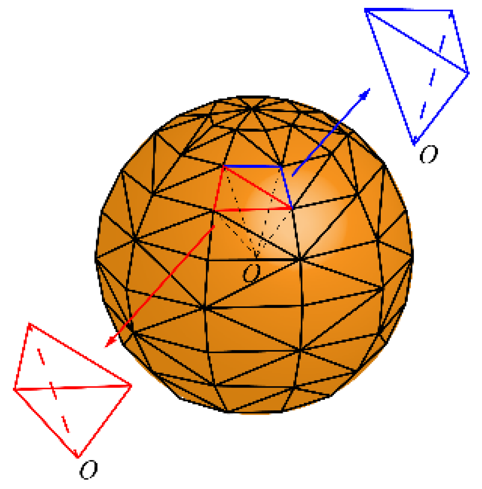
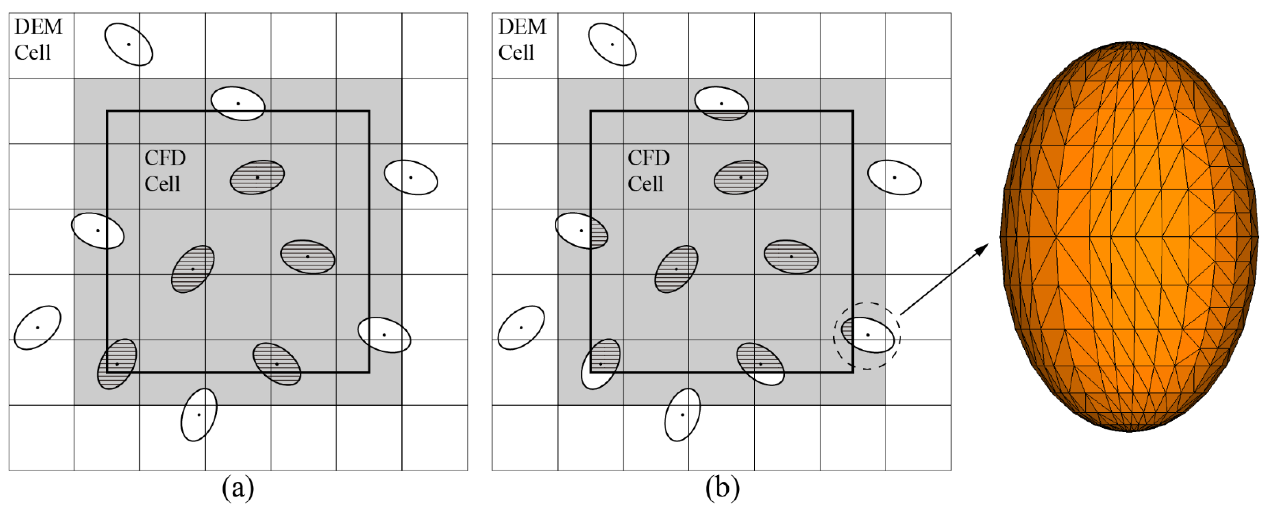
2.1. Particle Shape Representation Approach

The spherical approach and polyhedron approach are applied in this study to describe spherical particles and polyhedral particles, respectively. Polyhedral particles with triangular facets can be obtained by the import of their STL (Stereolithography) file. For a polyhedral particle with an arbitrary shape, the particle mass first needs to be detected. As mentioned above, the surfaces of the polyhedral particle are divided into many triangular facets. In order to detect the mass of the polyhedral particle, we choose a point in the particle randomly. With this point and the triangular facets, several tetrahedron elements can be obtained. The mass m_i of the tetrahedron element i can be acquired, and then the mass m of the polyhedral particle can be calculated by:

$$m={\displaystyle \sum _{i=1}^N{m}_i}$$

(1)

where N is the number of the tetrahedron elements. The particle’s mass center needs to be detected before simulation. The mass m_i and the mass center (x_i, y_i, z_i) of the tetrahedron element i can be obtained by the four vertexes of the tetrahedron, so the mass center (x₀, y₀, z₀) of the polyhedral particle can be obtained by:

$$x_0={\displaystyle \sum _{i=1}^N\frac{m_i{x}_i}{m}}$$

(2)

$$y_0={\displaystyle \sum _{i=1}^N\frac{m_i{y}_i}{m}}$$

(3)

$$z_0={\displaystyle \sum _{i=1}^N\frac{m_i{z}_i}{m}}$$

(4)

After the determination of mass center, the component tetrahedron elements of the polyhedral particle can be obtained, which are composed of the mass center and triangular facets. Taking a sphere as an example, a sphere with triangular facets can be seen in Figure 1. With these triangular facets and the mass center O, a sphere can be the composition of several component tetrahedron elements. Because of the complex shapes of polyhedral particles, a local coordinate system and a global coordinate system need to be employed to describe polyhedral particles accurately, which can have arbitrary positions and orientations. For example, in order to obtain the coordinate (x_j) of the vertex j in the global coordinate system, the vector (r_j) from the polyhedral particle’s mass center to the vertex j first needs to be detected in the local coordinate system. Then, with the coordinate (x_m) of the particle’s mass center in the global coordinate system and the transformation matrix A, the coordinate x_j can be calculated by:

$${\mathit{x}}_j={\mathit{x}}_m+\mathit{A}\cdot {\mathit{r}}_j$$

(5)

where A is the transformation matrix from the local coordinate system to the global coordinate system, which can be obtained from the Euler angles [2].

2.2. Particle Motion Equations

The motion of polyhedral particles includes translational and rotational motion, both of which obey Newton’s laws of motion. The motion equations can be formulated as:

$$m\frac{d\mathit{v}}{dt}={\displaystyle \sum {\mathit{F}}_c+{\mathit{F}}_d+{\mathit{F}}_b+m\mathit{g}}$$

(6)

$$\mathit{I}\frac{d\mathbf{\omega }}{dt}={\displaystyle \sum {\mathit{T}}_c}$$

(7)

where m is mass and I denotes the inertia tensor of polyhedral particle. v and ω are the particle translational velocity and particle rotational velocity, respectively. g is the gravitational acceleration. F_c, F_d and F_b are the contact force, the drag force and the buoyancy, respectively. The standard soft-sphere linear spring-dashpot model is applied to calculate the contact force, and the contact torque T_c can be obtained by these parameters [16,27].

The inertia tensor I of a polyhedral particle in the global coordinate system is time-varying because of the asymmetric structure and particle motion. As a result, the inertia tensor I must first be calculated to decide the rotational motion of a polyhedral particle. Similar to the calculation of mass m, the inertia tensor I′ of a polyhedral particle in the local coordinate system can be calculated according to its component tetrahedron elements. The moment of inertia I_xi′, I_yi′, and I_zi′ of the tetrahedron element i can be calculated by its density and volume, and the coordinates of the vertexes. Then, the moment of inertia in the local coordinate system can be written as:

$${\mathit{I}}_x^{\prime }={\displaystyle \sum _{i=1}^N{\mathit{I}}_{xi}^{\prime }}$$

(8)

$${\mathit{I}}_y^{\prime }={\displaystyle \sum _{i=1}^N{\mathit{I}}_{yi}^{\prime }}$$

(9)

$${\mathit{I}}_z^{\prime }={\displaystyle \sum _{i=1}^N{\mathit{I}}_{zi}^{\prime }}$$

(10)

where N is the total number of the tetrahedron elements.

What should be noted is that the inertia tensor I′ in the local coordinate system can transform to the inertia tensor I in the global coordinate system using the inverse matrix A.

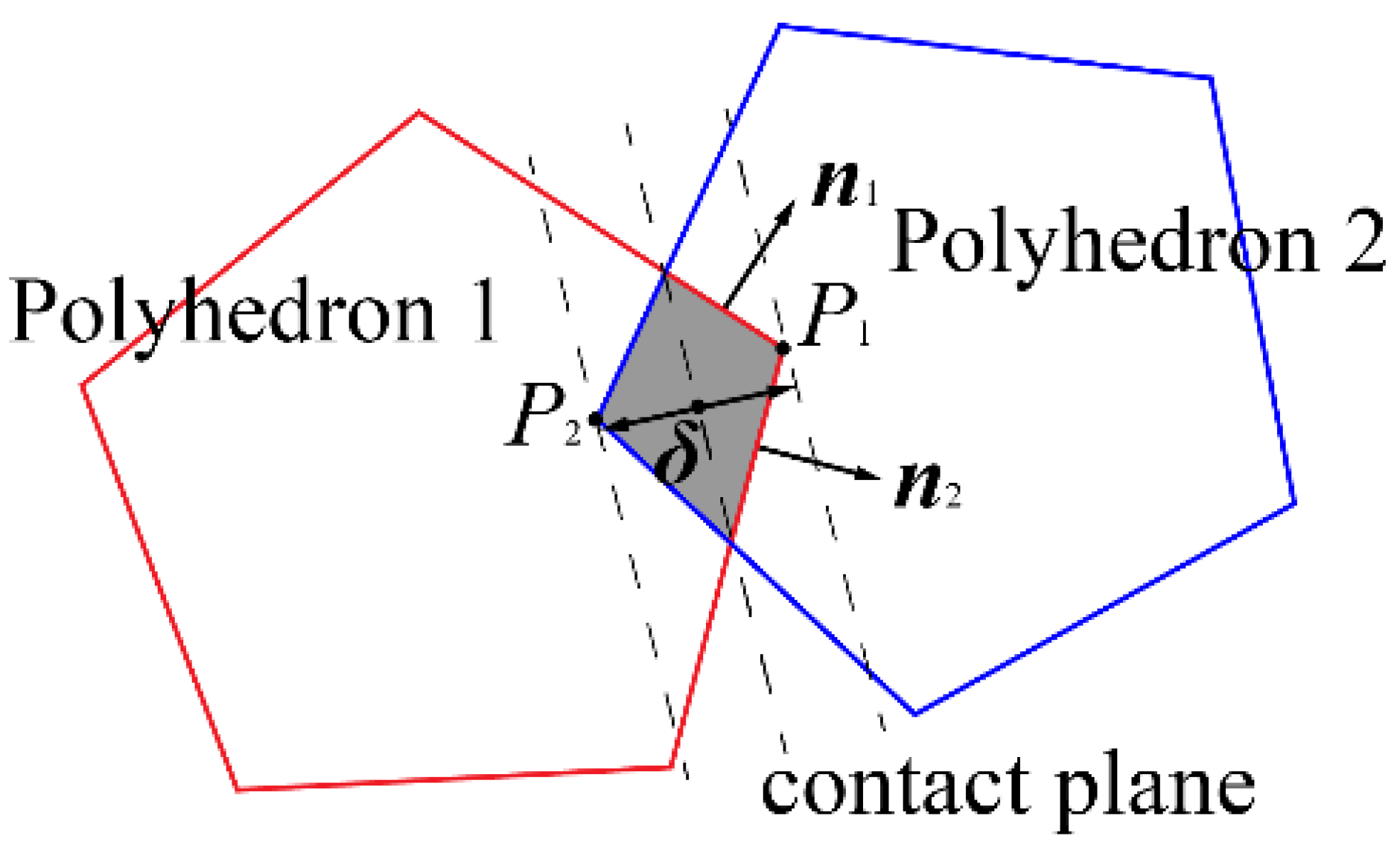
2.3. Contact Detection

The particles applied in this study are elastic and the contact interaction model of Feng et al. [23,41] is applied for contact detection with the polyhedron approach. The geometric features of a polyhedral particle include the vertexes, the edges connecting the vertexes, and the surfaces made up of edges. Because of the shape and the orientation of polyhedral particle, different contact types can be detected during the simulation, such as the contact between vertexes, the contact between vertex and surface, or the contact between some other geometric features of contacting polyhedral particles. A new polyhedron can be obtained in either contact type, which is the overlap of contacting polyhedral particles. This new polyhedron is called the overlap polyhedron in this study. Two simple polyhedral particles in contact with a typical contact type are chosen as an example, which is shown in Figure 2. The other contact types can be solved in a similar method. As Figure 2 shows, the overlap between two polyhedral particles forms a new polyhedron, P₁ and P₂ are the vertexes of Polyhedron 1 and Polyhedron 2, respectively. Naturally, the geometric features of the overlap polyhedron also include vertexes, edges, and facets, and all these features belong to the two contacting polyhedral particles. As shown in Figure 2, the features belonging to Polyhedron 1 are colored by red, and the other features belonging to Polyhedron 2 are colored by blue. In the overlap polyhedron, the outward normal unit vectors and areas of the facets belonging to Polyhedron 1 are n_i and A_i (i = 1, 2 in Figure 2), respectively. With these parameters, the normal unit vector of the overlap polyhedron n, which is normal to the contact plane, can be obtained by the sum of the unit normal vectors of the faces belonging to Polyhedron 1:

$$\mathit{n}={\displaystyle \sum A_i{n}_i}/\Vert A_i{n}_i\Vert$$

(11)

With the same method, n′, the sum of unit normal vectors of the facets belonging to Polyhedron 2, can also be calculated. As for the other contact types, the differences between them are that the overlap polyhedrons can be different. Different overlap polyhedrons correspond to different contact types. The determination of the geometric features involved in the contacted polyhedron is important to define the unit vectors n and n′, which can be vertexes, edges, and facets with different amounts for both contacting polyhedral particles. The volume of the overlap polyhedron and the unit normal vector n_i of each facet can be obtained with these geometric features.

The contact plane is perpendicular to the normal unit vector n and passes through the mass center of the overlap polyhedron, and the center of the overlap polyhedron is defined as the contact point. The combination method of the deepest-point method and polyhedron approach is applied to obtain the overlap δ. The deepest point in the overlap polyhedron is defined as the point of which the distance between this point and the contact plane has the maximum value on one side of the contact plane. After the detection of two deepest points in the overlap polyhedron on both sides of the contact plane, the overlap δ can be obtained by the distance between these two deepest points along the contact normal direction.

2.4. Fluid Motion Equations

The Navier-Stokes formulas are employed to describe the gas flow of a coupled gas-solid two-phase system. The equations of continuity and momentum conservation can be formulated as:

$$\frac{\partial }{\partial t}(\epsilon \rho )+\frac{\partial }{\partial x_j}(\epsilon \rho u_j)=0$$

(12)

$$\frac{\partial }{\partial t}(\epsilon \rho u_i)+\frac{\partial }{\partial x_j}(\epsilon \rho u_j{u}_i)=-\frac{\partial p}{\partial x_i}+\frac{\partial }{\partial x_j}\left[\epsilon \mu \left(\frac{\partial u_i}{\partial x_j}+\frac{\partial u_j}{\partial x_i}\right)\right]+{\mathit{F}}_s$$

(13)

where ρ, u, p, and µ denote the gas density, gas velocity, gas pressure, and gas viscosity, respectively. x is the coordinates. F_s represents the particle-fluid interaction force. The voidage fraction in the computational CFD cell is represented by ε, which can be stated as:

$$\epsilon =1-{\displaystyle \sum _{i=1}^n{V}_{p,i}/V_{cell}}$$

(14)

where n is the number of particles located in the CFD cell, V_p,i and V_cell are the volumes of particle i and the corresponding CFD cell, respectively.

As for the method of the calculation of the voidage fraction ε, some DEM cells will be associated with the CFD cell firstly, and only the particles residing in these DEM cells need to be considered, which can be seen in Figure 3a. The position of the mass center of the polyhedral particle is detected to determine if the polyhedral particle is in a computational CFD cell traditionally. Nevertheless, the accuracy of this algorithm is not high enough. With this method, if the particle mass center is in the CFD cell, the whole volume of the polyhedral particle will be applied to calculate the voidage fraction. As shown in Figure 3a, some particles are fully involved to calculate the voidage fraction when the mass centers of the particles are in the CFD cell. However, only some of them belong to this CFD cell. Additionally, some particles are not involved in the calculation of the voidage fraction when the mass centers of the particles are not in the CFD cell. However, some of them belong to this CFD cell. To solve this problem, we improved this search method. As mentioned above, an arbitrary polyhedral particle can be composed of several component tetrahedron elements with different amounts. Then, the mass center of each tetrahedron element is detected to decide if the tetrahedron element is in this CFD cell. By detecting the position of each component tetrahedron element rather than the whole particle, the calculation of the voidage fraction can be more accurate. The improved method of searching tetrahedron elements can be seen in Figure 3b. With this method, the voidage fraction can be calculated with part of the particle which is not fully involved in the CFD cell, and the computational accuracy can be improved. A similar method was used in our previous study with a good result [6].

2.5. Gas-Particle Interaction Force

Several types of interaction force are involved in the gas-particle system, and only buoyancy and drag force are emphasized in this study on account of the modest rotational and translational motion of polyhedral particles in the fluidized bed. The lift forces can be neglected because of the low gas velocity. Ignoring the influence of the circumambient particles, the formula of the drag force imposed on an individual particle can be written as:

$${\mathit{F}}_{d0}=\frac{1}{2}\rho {\epsilon }^2{C}_{D}A\left|\mathit{u}-\mathit{v}\right|\left(\mathit{u}-\mathit{v}\right)$$

(15)

where ε and C_D represent the voidage fraction and drag coefficient, respectively. u and v stand for the gas velocity and the particle velocity, respectively. A is the cross-sectional area of the sphere of which the volume is equal to the considered polyhedral particle.

In fact, the ambient particles will affect the drag force. As a result, Equation (15) was modified by Di Felice [52]:

$${\mathit{F}}_d={\mathit{F}}_{d0}{\epsilon }^{-(\chi +1)}$$

(16)

$$\chi =3.7-0.65\exp \left[-\frac{{\left(1.5-\log {\mathrm{Re}}_p\right)}^2}{2}\right]$$

(17)

$${\mathrm{Re}}_p=\frac{\epsilon \rho \left|\mathit{u}-\mathit{v}\right|d}{\mu }$$

(18)

where Re_p is the particle Reynolds number and d is the diameter of the sphere of which the volume is equal to the considered polyhedral particle.

Because of the complex shapes and non-symmetry of polyhedral particles, the calculation of drag force is much more complicated for polyhedral particles compared to spherical particles. Different drag force models have been devised for non-spherical particles. The Hölzer/Sommerfeld drag force model [29] is employed in this study to calculate the drag coefficient of polyhedral particles, which has been extensively applied in the simulation of the fluidization with non-spherical particles [6,33,34,35]. The Hölzer/Sommerfeld drag force model [29] can be formulated as:

$$C_D=\frac{8}{{\mathrm{Re}}_p}\frac{1}{\sqrt{{\varphi }_{\perp }}}+\frac{16}{{\mathrm{Re}}_p}\frac{1}{\sqrt{\varphi }}+\frac{3}{\sqrt{{\mathrm{Re}}_p}}\frac{1}{{\varphi }^{3/4}}+0.42\times {10}^{0.4{\left(-\log \varphi \right)}^{0.2}}\frac{1}{{\varphi }_{\perp }}$$

(19)

ϕ denotes the regular sphericity, which is the surface area ratio of the volume equivalent sphere to the corresponding particle. ϕ_⊥ represents the crosswise sphericity, which can be acquired by the area ratio of the cross section of the volume equivalent sphere to the projective plane of the corresponding particle against the direction of the fluid flow.

What should be noted is that in this study, the traditional drag force model is applied for spherical particles, which can be formulated as:

$$C_D=\{\begin{array}{cc}\frac{24}{{\mathrm{Re}}_p}\hfill & {\mathrm{Re}}_p\le 1\hfill \\ {\left(0.63+\frac{4.8}{{\mathrm{Re}}_p^{0.5}}\right)}^2\hfill & {\mathrm{Re}}_p>1\hfill \end{array}$$

(20)

The equation of the calculation of the buoyancy F_b can be calculated as:

$${\mathit{F}}_b=-\rho V_p\mathit{g}$$

(21)

where V_p is the volume of the corresponding particle.

After the calculations of the forces mentioned above, the gas-particle interaction force F_s in a CFD cell can be obtained as:

$${\mathit{F}}_s=\frac{-{\displaystyle \sum _{i=1}^n\left({\mathit{F}}_{d,i}+{\mathit{F}}_{b,i}\right)}}{V_{cell}}$$

(22)

where F_d,i and F_b,i represent the drag force and the buoyancy imposing on particle i, respectively. n is the number of the particles in the corresponding CFD cell.

3. Solution and Simulation Conditions

Four kinds of particles are adopted to investigate the fluidization of polyhedral particles in this study, which include spherical particles and three kinds of polyhedral particles. The governing equations are solved by the SIMPLEC method and the QUICK differencing scheme, and the fluid motion is solved by the pressure-based implicit integration method, which is solved by the software Fluent. As for the particle motion, it is solved by the linear spring-dashpot contact model and the explicit time integration method, which is realized through a self-developed DEM code (DEMSLab), and a coupling scheme is used between CFD and DEM. More detailed information of the CFD-DEM coupling method adopted in this study can be consulted in our previous studies [3,6,33].

The schematic diagram of the fluidized bed is shown in Figure 4. The sizes of the fluidized bed are 0.2 m, 0.03 m, and 1 m in width, thickness, and height, respectively. The fluid, which is air in this study, passes in from the bottom of the vessel along the direction of z-axis. The four side walls of the vessel are set to be stationary no-slip boundaries, which are the front, rear, right, and left walls. The size of the CFD mesh is 2 cm, 3 cm, and 2 cm in the x, y, and z directions, respectively. The polyhedral particles used in this study include one kind of pentahedron and two kinds of hexahedrons. The shape of the pentahedron is a triangular prism, of which the triangle faces are equilateral triangles, and the shapes of two hexahedrons are cuboids. These polyhedral particles are modeled by the polyhedron approach and the spherical particles are described by the spherical approach. The geometrical shapes of the polyhedral particles can be seen in Figure 5, which are named Polyhedron 1, Polyhedron 2, and Polyhedron 3, respectively. Their detailed geometric parameters are summarized in

Table 1. Particles used in experiments and CFD-DEM simulations.

Shape	Diameter (mm)	Length (mm)	Width (mm)	Height (mm)	Number
Sphere	6.8				3600
Polyhedron 1		8	8	6	3600
Polyhedron 2		5	5	6.5	3600
Polyhedron 3		4	4	10	3600

.

Particles are first dropped into the fluidized bed under gravity. All particles are packed with random locations and orientations, and the initial kinetic energies are all zero, allowing free fall and random packing. A total of 3600 particles are applied for each case. The four kinds of particles have the same densities (480 kg/m³), and their equivalent diameters are 6.8 mm. Both the frictional coefficient and the restitution coefficient between particles are 0.5. The restitution coefficient between particle and wall is 0.5 and the frictional coefficient is 0.4. The air flow into the model from the end of the vessel and the superficial velocity starts from 0.4 m/s and ends at 2.0 m/s, of which the step is 0.1 m/s. What should be noted is that the superficial velocity is fixed during each simulation. The time step is 8 × 10⁻⁶ s and the detailed parameters are listed in

Table 2. Parameters used in the simulations and experiments.

Parameters	Value
Particle number	3600
Particle density (kg/m3)	480
Fluidized bed dimensions (m) (width × thickness × height)	0.2 × 0.03 × 1.0
Restitution coefficient	0.5
Friction coefficient between particles	0.5
Friction coefficient between particle and wall	0.4
Gas density (kg/m3)	1.225
Gas viscosity (Pa·s)	1.79 × 10−5
DEM time step (s)	8 × 10−6
CFD time step (s)	4 × 10−5

.

4. Validation and Discussion

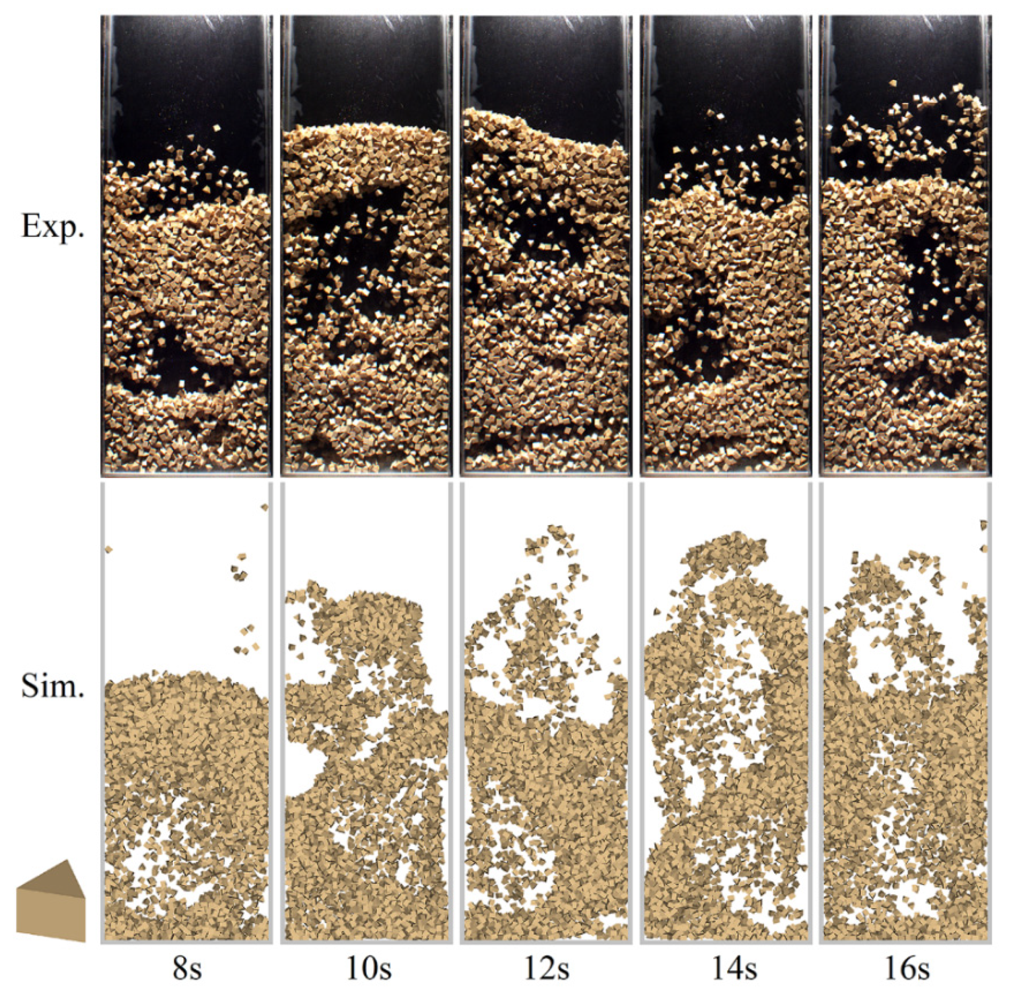
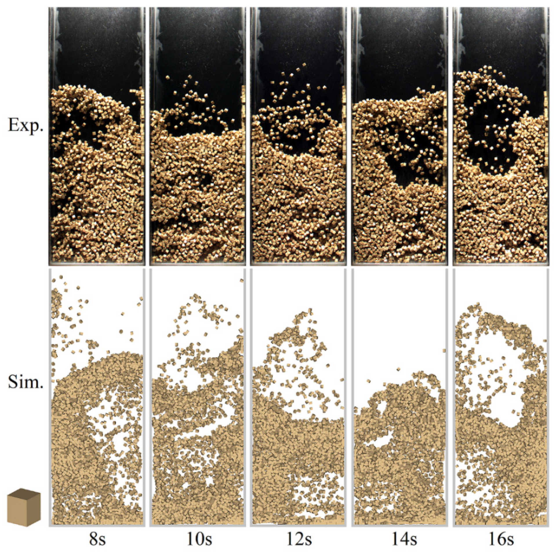
4.1. Validation of the CFD-DEM Model

Corresponding fluidized bed experiments of polyhedral particles are carried out to validate our CFD-DEM model. The sizes of the equipment are same as the simulations, of which the dimensions are 0.2 × 0.03 × 1.0 m (width × thickness × height). The walls of the vessel are made of the transparent polymethyl methacrylate and a high-speed camera is placed in front of the vessel to capture the behaviors of the polyhedral particles during experiments. The gas flow rate is measured with a vortex shedding flowmeter. In order to assure an even gas flow, a porous gas distributor with 20% gas passage is installed at the bottom of the vessel. The pressure drop is measured by two pressure tapping points, one point is set near the outlet and the other one is slightly under the gas distributor. Corresponding simulations are carried out for the validation of the CFD-DEM model. The parameters used in these simulations can be seen in Table 2.

Figure 5 presents the snapshots of the initial packed bed in simulations and experiments, and the heights of the initial packed beds are nearly the same between experiments and corresponding simulations. Some snapshots during the experiments and simulations of three kinds of polyhedral particles can be seen in Figure 6, Figure 7 and Figure 8, of which the gas superficial velocity is 1.6 m/s. The simulated flow behaviors of different polyhedral particles can be seen are similar as the corresponding experiments with reasonable accuracy from visual observation. For further validation, the pressure drops changing with the superficial velocity are compared between experiments and simulations. As shown in Figure 9, the results calculated from simulations match well with the pressure drops of corresponding experiments. As for the minimum fluidization velocity, it also presents good agreement with comparative accuracy between simulations and corresponding experiments. The range of the minimum fluidization velocities can be found is between 0.8 m/s and 1.0 m/s for all simulations and experiments, which predicts well between the experiments and the corresponding simulations.

Furthermore, the time-averaged bed heights of three polyhedral particles during 8–16 s can be seen in Figure 10, and the superficial velocities are 1.6 m/s and 1.8 m/s, respectively. The time-based standard deviations of heights are denoted by the error bars. The method of Mahajan et al. [53] is employed to calculate the bed height in this study. From Figure 10 we can see that the time-averaged bed heights become higher for all three kinds of polyhedral particles as the gas superficial velocity increases. In general, the time-averaged bed heights of experiments are comparable with corresponding simulations. As a result, the above results indicate that the CFD-DEM coupling method can predict the behaviors of polyhedral particles with reasonable accuracy.

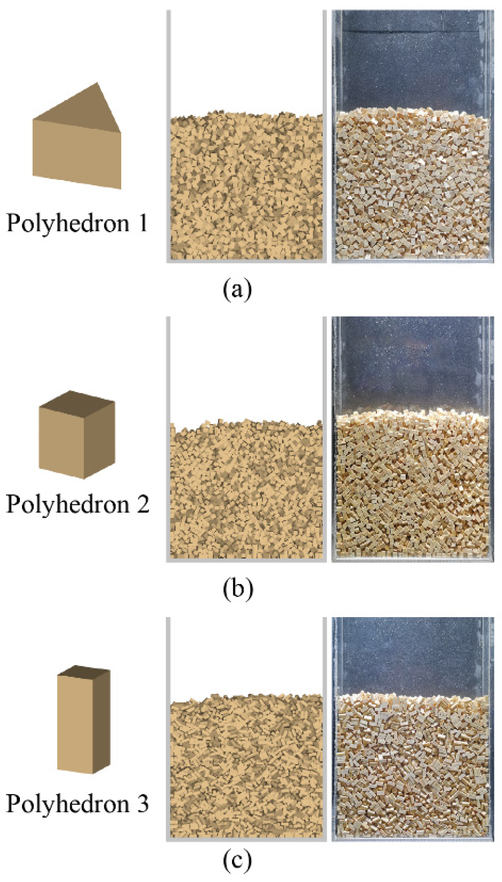
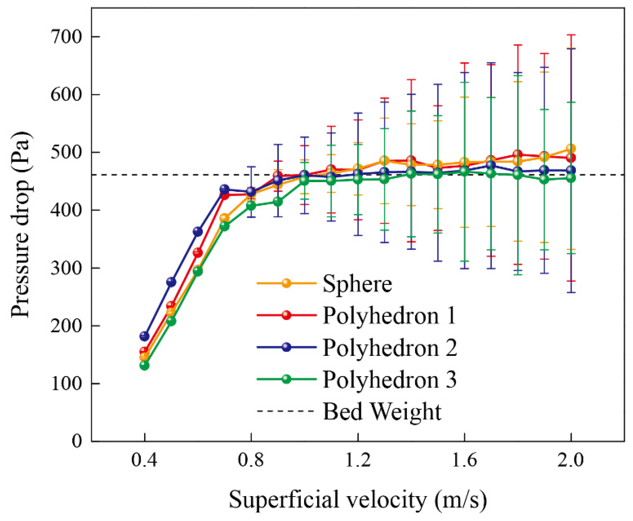
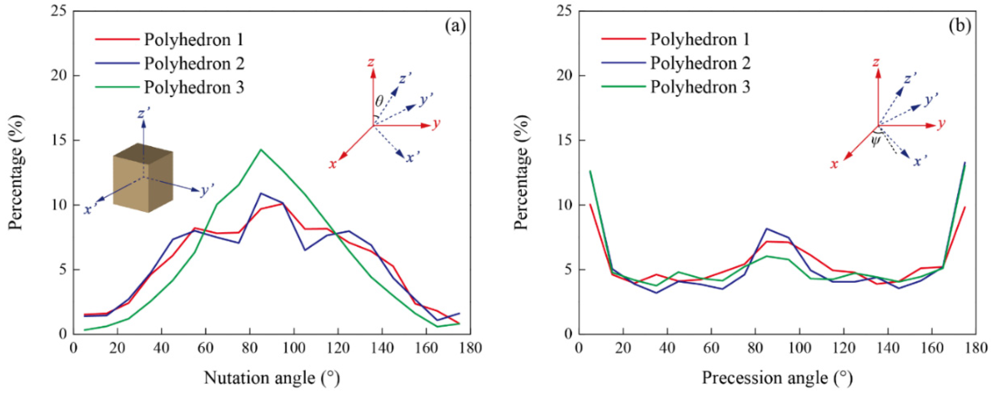
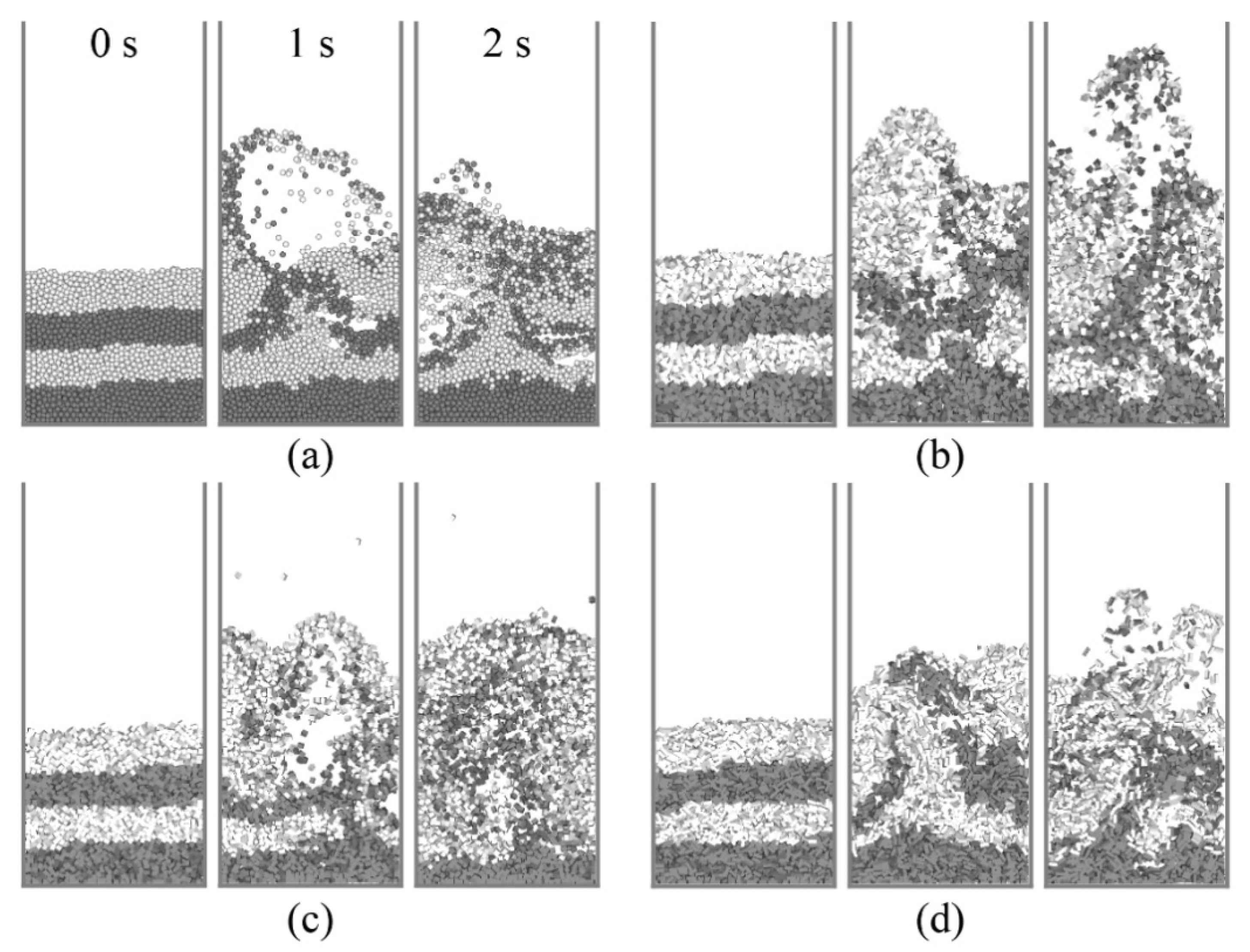
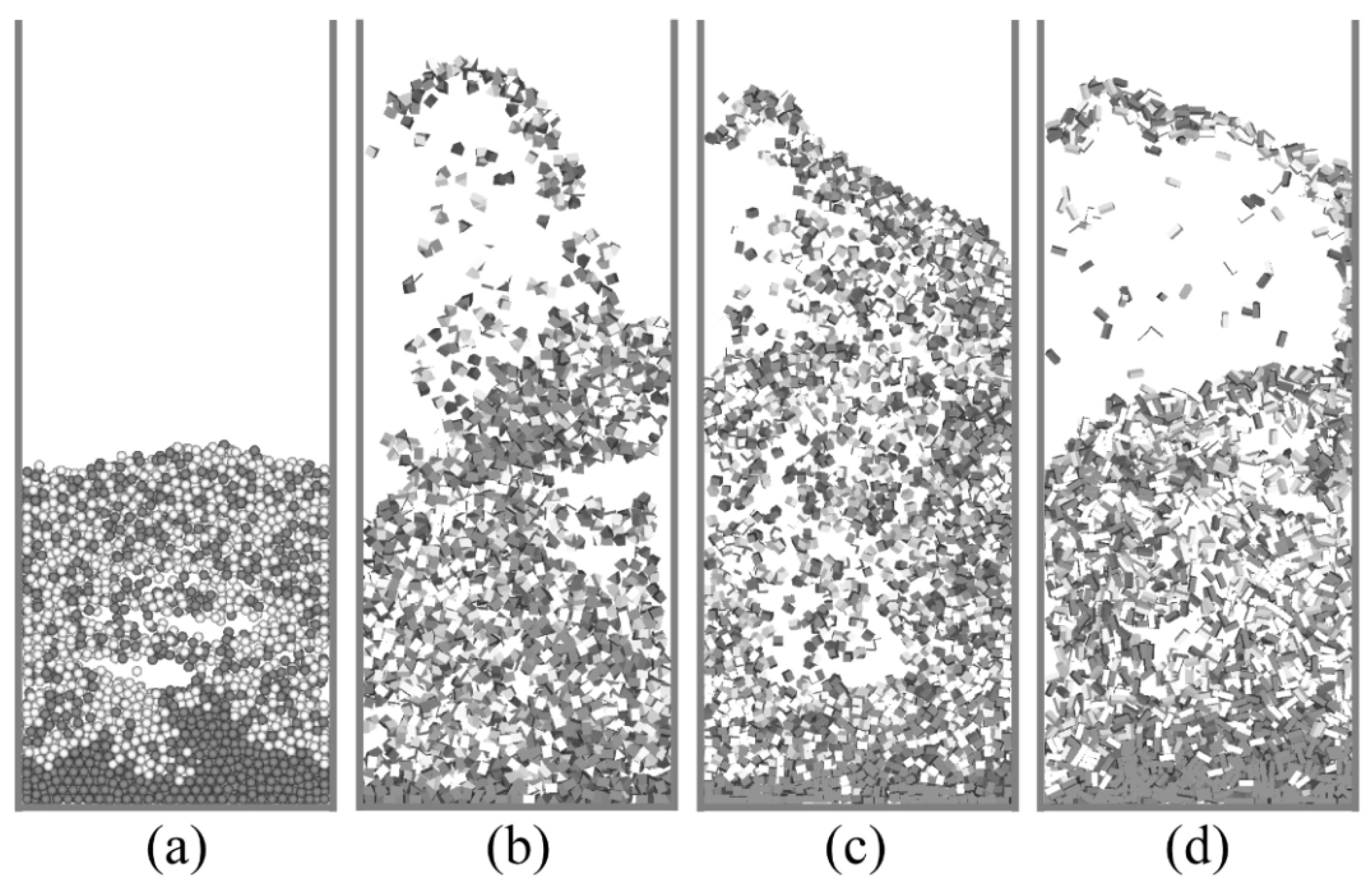
4.2. Fluidization Behaviors of Different Particles

Besides the simulations mentioned above, the simulations of the fluidization with the volume equivalent sphere are also included for the purpose of comparison. Figure 11 shows the initial packed beds of four kinds of particles, we can see that the fill height of Polyhedron 1 is the highest of the four packed beds and the height of Polyhedron 3 is the second highest. The fill heights and the voidage fractions are listed in

Table 3. The fill height (mm), voidage fraction, and surface area (mm²) for all kinds of particles.

	Sphere	Polyhedron 1	Polyhedron 2	Polyhedron 3
Fill height (mm)	171.74	189.76	176.19	182.93
Voidage fraction	0.425	0.474	0.447	0.475
Surface area (mm2)	145.27	199.43	147.5	152

. For Polyhedron 1, its shape is a triangular prism, which is more irregular than the other two cuboid polyhedral particles. As such, for the initial pack, the void fraction of Polyhedron 1 is higher than the others, and the fill height is the highest. As for Polyhedron 2 and Polyhedron 3, the aspect ratio of Polyhedron 3, which is defined as the length ratio of the height to width in this study, is larger than that of Polyhedron 2. As a result, the void fraction of Polyhedron 3 is larger than Polyhedron 2, which leads to a higher fill height for Polyhedron 3 compared to Polyhedron 2.

Figure 12 shows the pressure drops of four particles which change with the superficial velocity, and the error bar denotes the time-based standard deviation of the pressure drop. It is generally known that during the packed bed stage, the fluidized bed keeps stable and the pressure drop has little fluctuation. As the gas superficial velocity increases, the fluidized bed starts to expand and bubbles will occur in the incipient fluidization stage, which leads to a strong fluctuation of pressure drop. From Figure 12, the minimum fluidization velocities of all kinds of particles can be acquired, and the differences of the minimum fluidization velocity between Polyhedral 1 and Polyhedron 2 are small. The minimum fluidization velocity of Polyhedron 3 is a little larger than the velocities of Polyhedron 1 and Polyhedron 2.

According to Equations (15)–(17), it is clear that decreasing the bed voidage fraction and increasing the projected face area will cause the increase of drag force, and the particle motion can be promoted at last. For the particles mentioned above, the voidage fractions in the packed bed are summarized in Table 3. The orientation of non-spherical particles has influence on the projected face area. In this study, the Euler angles are employed to describe particle orientation. The angle between the z-axis and z′-axis is the nutation angle (θ), which can be seen in the inset of Figure 13a. The angle between the x-axis and the intersection line between the x-y plane and x′-y′ plane is the precession angle (ψ), which can be seen in the inset of Figure 13b.The ranges of the nutation angle and precession angle are both 0°–180° because of the symmetry of polyhedrons. Figure 13 shows the distributions of the nutation angle and precession angle of three polyhedrons in the packed bed. It can be seen that the orientations are similar on all three polyhedrons in the packed bed, so the surface areas in Table 3 can be used to indicate the differences of the projected face areas between these polyhedrons. As shown in Table 3, because of the relatively large voidage fraction and small surface area, the minimum fluidization velocity of Polyhedron 3 is a little higher compared to Polyhedron 1 and Polyhedron 2.

As for the differences between polyhedral particles and spherical particles, particle shape can have influence on the motion of different particles and Figure 14 shows the snapshots of the behaviors of these four kinds of particles at 1.2 m/s, in which the snapshots are obtained at the same time for each case respectively. It can be seen that more bubbles appear and bed heights are higher for polyhedral particles when comparing with spherical particles, especially for Polyhedron 1. In other words, the motion of Polyhedron 1 is stronger than spherical particles at the same superficial velocity. It can be seen from Table 3 that the surface area of Polyhedron 1 is much higher than the surface area of the spherical particle, which could be the cause of the stronger motion of Polyhedron 1 compared to the spherical particles at the same superficial velocity.

4.3. Particle Mixing in the Fluidized Bed

Understanding the behaviors of particle mixing is important for relevant processes. Figure 14 presents the snapshots of particle behaviors for spheres, Polyhedron 1, Polyhedron 2, and Polyhedron 3, respectively, of which the superficial velocity is 1.2 m/s. The fluidized bed is divided into four equal parts along the direction of the z-axis, of which different parts are colored by black and white. It is clear that polyhedral particles have a higher mixing degree than the spherical particles at the same superficial velocity. This is because particle orientation has an influence on polyhedral particles but spheres are not influenced by orientation. As a result, the particle fluid forces change more drastically for polyhedral particles compared to spheres, which can cause higher mixing degrees [7,46,47].

Although the particles at the bottom of the bed form a cluster and have a tendency to rise, some particles at the bottom of the vessel nearly do not move up at all. This is particularly obvious for the spherical particles in Figure 14a. Figure 15 shows the snapshots of the particle behaviors at 8 s for all four kinds of particles, of which the superficial velocity is 1.2 m/s. It is clear that spherical particles have a minimum mixing degree visually. As shown in Figure 15, for spherical particles, there are more black particles still staying at the bottom of the bed. For the three kinds of polyhedral particles, particles in black stay at the bottom of the bed in various degrees, and for Polyhedron 3 this degree is a little larger than the degrees of Polyhedron 1 and Polyhedron 2, visually. More black particles can be seen in the upside of the bed for Polyhedron 1 and Polyhedron 2.

To further investigate the particle mixing, the fluidized bed is divided into two equal parts along the direction of the z-axis, as shown in the inset of Figure 16a. The Lacey mixing index [54] is employed to quantify the mixing process. Figure 16a shows the variation of the mixing index changing with time for all kinds of particles of which the superficial velocity is 1.2 m/s. As mentioned above, the mixing degree of spherical particles is the lowest among these four kinds of particles, which can also be observed from Figure 16a. The mixing degree of Polyhedron 3 is a little lower than the mixing degrees of Polyhedron 1 and Polyhedron 2. The mixing degree is influenced by particle motion. As a result, the spherical particles demonstrate a lower mixing degree because of their more evenly distributed forces. Furthermore, Figure 16b shows the variation between the Lacey mixing index and the time while the superficial velocity is 1.6 m/s. At the beginning of the process, the mixing degrees of all kinds of particles are almost equal because of the strong particle motion caused by the sudden high superficial velocity. As the simulations continue, the mixing degree of spherical particles remains lower than the mixing degrees of the other three polyhedral particles.

5. Conclusions

In this study, a numerical CFD-DEM investigation of polyhedral particles described by the polyhedron approach in a fluidized bed is studied. The mass and the inertia tensor of a polyhedral particle can be calculated by the accumulation of the masses and the inertia tensors of its tetrahedron elements. Contact detection with the polyhedron approach is based on the combination of the overlapping volume method and the deepest point method. The tetrahedron elements of the polyhedral particle are applied to calculate the voidage fraction. Based on the comparison results between experiments and corresponding simulations, the established CFD-DEM method for the polyhedron approach can reproduce the fluidization of polyhedral particles with reasonable accuracy. The fluidization behaviors of polyhedral particles are also investigated with this CFD-DEM method. Comparing with spherical particles, the motion for polyhedral particles is stronger and the mixing degree is higher under the same fluidization gas velocity. In summary, this study provides an effective CFD-DEM coupling method for the polyhedron approach which can be applied for future investigations involving the fluidization of non-spherical particles encountered in industrial applications.

References

1. Azmir, J.; Hou, Q.; Yu, A. CFD-DEM simulation of drying of food grains with particle shrinkage. Powder Technol. 2019, 343, 792–802. [Google Scholar] [CrossRef]
2. Zhong, W.; Yu, A.; Liu, X.; Tong, Z.; Zhang, H. DEM/CFD-DEM Modelling of Non-spherical Particulate Systems: Theoretical Developments and Applications. Powder Technol. 2016, 302, 108–152. [Google Scholar] [CrossRef]
3. Ma, H.; Xu, L.; Zhao, Y. CFD-DEM simulation of fluidization of rod-like particles in a fluidized bed. Powder Technol. 2017, 314, 355–366. [Google Scholar] [CrossRef]
4. Höhner, D.; Wirtz, S.; Kruggel-Emden, H.; Scherer, V. Comparison of the multi-sphere and polyhedral approach to simulate non-spherical particles within the discrete element method: Influence on temporal force evolution for multiple contacts. Powder Technol. 2011, 208, 643–656. [Google Scholar] [CrossRef]
5. Zhou, Y.; Zhou, B.; Li, J.; Wang, H. Study on the Multi-sphere Method Modeling the 3D Particle Morphology in DEM. Springer Proc. Phys. 2017, 188, 601–608. [Google Scholar] [CrossRef]
6. Ma, H.; Zhao, Y.; Cheng, Y. CFD-DEM modeling of rod-like particles in a fluidized bed with complex geometry. Powder Technol. 2019, 344, 673–683. [Google Scholar] [CrossRef]
7. Vollmari, K.; Oschmann, T.; Kruggel-Emden, H. Mixing quality in mono- and bidisperse systems under the influence of particle shape: A numerical and experimental study. Powder Technol. 2017, 308, 101–113. [Google Scholar] [CrossRef]
8. Chang, J.; Wang, G.; Gao, J.; Zhang, K.; Chen, H.; Yang, Y. CFD modeling of particle–particle heat transfer in dense gas-solid fluidized beds of binary mixture. Powder Technol. 2012, 217, 50–60. [Google Scholar] [CrossRef]
9. Lu, G.; Third, J.; Müller, C. Discrete element models for non-spherical particle systems: From theoretical developments to applications. Chem. Eng. Sci. 2015, 127, 425–465. [Google Scholar] [CrossRef]
10. Cundall, P.A.; Strack, O.D.L. A discrete numerical model for granular assemblies. Géotechnique 1979, 29, 47–65. [Google Scholar] [CrossRef]
11. Tsuji, Y.; Kawaguchi, T.; Tanaka, T. Discrete particle simulation of two-dimensional fluidized bed. Powder Technol. 1993, 77, 79–87. [Google Scholar] [CrossRef]
12. Kruggel-Emden, H.; Rickelt, S.; Wirtz, S.; Scherer, V. A study on the validity of the multi-sphere Discrete Element Method. Powder Technol. 2008, 188, 153–165. [Google Scholar] [CrossRef]
13. Lin, X.; Ng, T.-T. Contact detection algorithms for three-dimensional ellipsoids in discrete element modelling. Int. J. Numer. Anal. Methods Géoméch. 1995, 19, 653–659. [Google Scholar] [CrossRef]
14. Yan, B.; Regueiro, R.A.; Sture, S. Three-dimensional ellipsoidal discrete element modeling of granular materials and its coupling with finite element facets. Eng. Comput. 2010, 27, 519–550. [Google Scholar] [CrossRef]
15. Mola, I.; Yu, A.; Zhou, Z. Particle scale modelling of mixing of ellipsoids and spheres in gas-fluidized beds by a modified drag correlation. Powder Technol. 2019, 343, 619–628. [Google Scholar] [CrossRef]
16. You, Y.; Liu, M.; Ma, H.; Xu, L.; Liu, B.; Shao, Y.; Tang, Y.; Zhao, Y. Investigation of the vibration sorting of non-spherical particles based on DEM simulation. Powder Technol. 2018, 325, 316–332. [Google Scholar] [CrossRef]
17. Ma, H.; Zhao, Y. Modelling of the flow of ellipsoidal particles in a horizontal rotating drum based on DEM simulation. Chem. Eng. Sci. 2017, 172, 636–651. [Google Scholar] [CrossRef]
18. Zhao, Y.; Xu, L.; Umbanhowar, P.B.; Lueptow, R.M. Discrete element simulation of cylindrical particles using super-ellipsoids. Particuology 2019, 46, 55–66. [Google Scholar] [CrossRef]
19. Govender, N.; Wilke, D.N.; Kok, S. Collision detection of convex polyhedra on the NVIDIA GPU architecture for the discrete element method. Appl. Math. Comput. 2015, 267, 810–829. [Google Scholar] [CrossRef]
20. Govender, N.; Rajamani, R.; Wilke, D.; Wu, C.-Y.; Khinast, J.; Glasser, B.J. Effect of particle shape in grinding mills using a GPU based DEM code. Miner. Eng. 2018, 129, 71–84. [Google Scholar] [CrossRef] [Green Version]
21. Höhner, D.; Wirtz, S.; Scherer, V. Experimental and numerical investigation on the influence of particle shape and shape approximation on hopper discharge using the discrete element method. Powder Technol. 2013, 235, 614–627. [Google Scholar] [CrossRef]
22. Smeets, B.; Odenthal, T.; Vanmaercke, S.; Ramon, H. Polygon-based contact description for modeling arbitrary polyhedra in the Discrete Element Method. Comput. Methods Appl. Mech. Eng. 2015, 290, 277–289. [Google Scholar] [CrossRef] [Green Version]
23. Xie, C.; Song, T.; Zhao, Y. Discrete element modeling and simulation of non-spherical particles using polyhedrons and super-ellipsoids. Powder Technol. 2020, 368, 253–267. [Google Scholar] [CrossRef]
24. Freireich, B.; Kumar, R.; Ketterhagen, W.; Su, K.; Wassgren, C.; Zeitler, A. Comparisons of intra-tablet coating variability using DEM simulations, asymptotic limit models, and experiments. Chem. Eng. Sci. 2015, 131, 197–212. [Google Scholar] [CrossRef] [Green Version]
25. Tao, H.; Jin, B.; Zhong, W.; Wang, X.; Ren, B.; Zhang, Y.; Xiao, R. Discrete element method modeling of non-spherical granular flow in rectangular hopper. Chem. Eng. Process. Process. Intensif. 2010, 49, 151–158. [Google Scholar] [CrossRef]
26. Markauskas, D.; Kačianauskas, R.; Džiugys, A.; Navakas, R. Investigation of adequacy of multi-sphere approximation of elliptical particles for DEM simulations. Granul. Matter 2009, 12, 107–123. [Google Scholar] [CrossRef]
27. Liu, Z.; Zhao, Y. Multi-super-ellipsoid model for non-spherical particles in DEM simulation. Powder Technol. 2020, 361, 190–202. [Google Scholar] [CrossRef]
28. Liu, Z.; Ma, H.; Zhao, Y. Comparative study of discrete element modeling of tablets using multi-spheres, multi-super-ellipsoids, and polyhedrons. Powder Technol. 2021, 390, 34–49. [Google Scholar] [CrossRef]
29. Hölzer, A.; Sommerfeld, M. New simple correlation formula for the drag coefficient of non-spherical particles. Powder Technol. 2008, 184, 361–365. [Google Scholar] [CrossRef]
30. Haider, A.; Levenspiel, O. Drag coefficient and terminal velocity of spherical and nonspherical particles. Powder Technol. 1989, 58, 63–70. [Google Scholar] [CrossRef]
31. Tran-Cong, S.; Gay, M.; Michaelides, E.E. Drag coefficients of irregularly shaped particles. Powder Technol. 2004, 139, 21–32. [Google Scholar] [CrossRef]
32. Ganser, G.H. A rational approach to drag prediction of spherical and nonspherical particles. Powder Technol. 1993, 77, 143–152. [Google Scholar] [CrossRef]
33. Ma, H.; Zhao, Y. Investigating the fluidization of disk-like particles in a fluidized bed using CFD-DEM simulation. Adv. Powder Technol. 2018, 29, 2380–2393. [Google Scholar] [CrossRef]
34. Liu, X.; Gan, J.; Zhong, W.; Yu, A. Particle shape effects on dynamic behaviors in a spouted bed: CFD-DEM study. Powder Technol. 2020, 361, 349–362. [Google Scholar] [CrossRef]
35. Farivar, F.; Zhang, H.; Tian, Z.F.; Gupte, A. CFD-DEM -DDM Model for Spray Coating Process in a Wurster Coater. J. Pharm. Sci. 2020, 109, 3678–3689. [Google Scholar] [CrossRef]
36. Cundall, P. Formulation of a three-dimensional distinct element model—Part I. A scheme to detect and represent contacts in a system composed of many polyhedral blocks. Int. J. Rock Mech. Min. Sci. Géoméch. Abstr. 1988, 25, 107–116. [Google Scholar] [CrossRef]
37. Nezami, E.G.; Hashash, Y.M.; Zhao, D.; Ghaboussi, J. A fast contact detection algorithm for 3-D discrete element method. Comput. Geotech. 2004, 31, 575–587. [Google Scholar] [CrossRef]
38. Nezami, E.G.; Hashash, Y.M.A.; Zhao, D.; Ghaboussi, J. Shortest link method for contact detection in discrete element method. Int. J. Numer. Anal. Methods Géoméch. 2006, 30, 783–801. [Google Scholar] [CrossRef]
39. Dong, K.; Wang, C.; Yu, A. A novel method based on orientation discretization for discrete element modeling of non-spherical particles. Chem. Eng. Sci. 2015, 126, 500–516. [Google Scholar] [CrossRef]
40. Boon, C.; Houlsby, G.; Utili, S. A new algorithm for contact detection between convex polygonal and polyhedral particles in the discrete element method. Comput. Geotech. 2012, 44, 73–82. [Google Scholar] [CrossRef]
41. Feng, Y.; Han, K.; Owen, D. Energy-conserving contact interaction models for arbitrarily shaped discrete elements. Comput. Methods Appl. Mech. Eng. 2012, 205–208, 169–177. [Google Scholar] [CrossRef]
42. Fraige, F.Y.; Langston, P.A.; Chen, G. Distinct element modelling of cubic particle packing and flow. Powder Technol. 2008, 186, 224–240. [Google Scholar] [CrossRef]
43. Mack, S.; Langston, P.; Webb, C.; York, T. Experimental validation of polyhedral discrete element model. Powder Technol. 2011, 214, 431–442. [Google Scholar] [CrossRef]
44. Liu, L.; Ji, S. Bond and fracture model in dilated polyhedral DEM and its application to simulate breakage of brittle materials. Granul. Matter 2019, 21, 41. [Google Scholar] [CrossRef]
45. Govender, N.; Wilke, D.; Pizette, P.; Abriak, N.-E. A study of shape non-uniformity and poly-dispersity in hopper discharge of spherical and polyhedral particle systems using the Blaze-DEM GPU code. Appl. Math. Comput. 2018, 319, 318–336. [Google Scholar] [CrossRef]
46. Oschmann, T.; Hold, J.; Kruggel-Emden, H. Numerical investigation of mixing and orientation of non-spherical particles in a model type fluidized bed. Powder Technol. 2014, 258, 304–323. [Google Scholar] [CrossRef]
47. Oschmann, T.; Vollmari, K.; Kruggel-Emden, H.; Wirtz, S. Numerical Investigation of the Mixing of Non-spherical Particles in Fluidized Beds and during Pneumatic Conveying. Procedia Eng. 2015, 102, 976–985. [Google Scholar] [CrossRef] [Green Version]
48. Vollmari, K.; Jasevičius, R.; Kruggel-Emden, H. Experimental and numerical study of fluidization and pressure drop of spherical and non-spherical particles in a model scale fluidized bed. Powder Technol. 2016, 291, 506–521. [Google Scholar] [CrossRef]
49. Xiong, H.; Wu, H.; Bao, X.; Fei, J. Investigating effect of particle shape on suffusion by CFD-DEM modeling. Constr. Build. Mater. 2021, 289, 123043. [Google Scholar] [CrossRef]
50. Tang, C.; Yang, Y.-C.; Liu, P.-Z.; Kim, Y.-J. Prediction of Abrasive and Impact Wear Due to Multi-Shaped Particles in a Centrifugal Pump via CFD-DEM Coupling Method. Energies 2021, 14, 2391. [Google Scholar] [CrossRef]
51. Zhou, J.W.; Liu, Y.; Liu, S.Y.; Du, C.L.; Li, J.P. Effects of particle shape and swirling intensity on elbow erosion in dilute-phase pneumatic conveying. Wear 2017, 380, 66–77. [Google Scholar] [CrossRef]
52. Di Felice, R. The voidage function for fluid-particle interaction systems. Int. J. Multiph. Flow 1994, 20, 153–159. [Google Scholar] [CrossRef]
53. Mahajan, V.V.; Padding, J.T.; Nijssen, T.M.J.; Buist, K.A.; Kuipers, J.A.M. Nonspherical particles in a pseudo-2D fluidized bed: Experimental study. Part. Technol. Fluid. 2018, 64, 1573–1590. [Google Scholar] [CrossRef] [PubMed]
54. Lacey, P.M.C. Developments in the theory of particle mixing. J. Appl. Chem. 2007, 4, 257–268. [Google Scholar] [CrossRef]
Figure 1. Sphere described by the polyhedron model with tetrahedron elements.
Energies 14 04939 g001
Figure 2. Contact detection between polyhedral particles.
Energies 14 04939 g002
Figure 3. The method of calculating the voidage fraction in a CFD cell: (a) traditional method of searching particles, and (b) improved method of searching tetrahedron elements.
Energies 14 04939 g003
Figure 4. The schematic diagram of the fluidized bed applied in this study.
Energies 14 04939 g004
Figure 5. The snapshots of the initial packed bed in simulations and experiments. (a)Polyhedron 1, (b) Polyhedron 2, (c) Polyhedron 3.
Energies 14 04939 g005
Figure 6. The snapshots during experiments and simulations for Polyhedron 1 when the superficial velocity is 1.6 m/s.
Energies 14 04939 g006
Figure 7. The snapshots during experiments and simulations for Polyhedron 2 when the superficial velocity is 1.6 m/s.
Energies 14 04939 g007
Figure 8. The snapshots during experiments and simulations for Polyhedron 3 when the superficial velocity is 1.6 m/s.
Energies 14 04939 g008
Figure 9. Pressure drops obtained from experiments and simulations at different superficial velocities for polyhedral particles: (a) Polyhedron 1, (b) Polyhedron 2, and (c) Polyhedron 3.
Energies 14 04939 g009
Figure 10. The time-averaged bed heights obtained from experiments and simulations during 8–16 s at 1.6 m/s and 1.8 m/s (error bars denote the time-based standard deviations of the fluidization bed heights).
Energies 14 04939 g010
Figure 11. The initial packed beds of four kinds of particles: (a) Sphere, (b) Polyhedron 1, (c) Polyhedron 2, and (d) Polyhedron 3.
Energies 14 04939 g011
Figure 12. The pressure drops at different gas superficial velocities for all four kinds of particles (error bars indicate the time-based standard deviation of the pressure drop fluctuation).
Energies 14 04939 g012
Figure 13. Distribution of the orientation for three kinds of polyhedrons in the packed bed: (a) nutation angle, and (b) precession angle.
Energies 14 04939 g013
Figure 14. Snapshots of particle behaviors at 1.2 m/s (fluidized bed is divided into four equal parts along the z-direction colored by black and white): (a) Sphere, (b) Polyhedron 1, (c) Polyhedron 2, and (d) Polyhedron 3.
Energies 14 04939 g014
Figure 15. Snapshots of particle behaviors at 8s while the superficial velocity is 1.2 m/s for all kinds of particles: (a) Sphere, (b) Polyhedron 1, (c) Polyhedron 2, and (d) Polyhedron 3.
Energies 14 04939 g015
Figure 16. The Lacey mixing index for all four kinds of particles (fluidized bed is divided into two equal parts along the z-direction by different color): (a) the superficial velocity is 1.2 m/s, and (b) the superficial velocity is 1.6 m/s.
Energies 14 04939 g016