Stochastic Modelling to Analyze the Impact of Electric Vehicle Penetration in Thailand

Abstract

Electric Vehicle (EV) technology is one of the most promising solutions to reduce dependence on fossil fuels and greenhouse gas (GHG) emissions in the transportation sector. However, a large increase of EVs raises concerns about negative impacts on electricity generation, transmission, and distribution systems. This study analyzes the benefits and trade-offs for EV penetration in Thai road transport based on EV penetration scenarios from 2019 to 2036. Two charging strategies are considered to assess the impact of EV charging: free charging and off-peak charging. Uncertainty variables are considered by a stochastic approach based on Monte-Carlo simulation (MCS). The simulation results shown that the adoption of EVs can reduce both energy consumption and GHG emissions. The results also indicate that the increased load due to EV charging demand in all scenarios is still within the buffer level, compared to the installed generation capacity in the Power Development Plan 2018 revision 1 (PDP2018r1), and the off-peak charging strategy is more beneficial than the free-charging strategy. However, the increased load demand caused by all EV charging strategies has a direct impact on the power generating schedule, and also decreases the system reliability level.

1. Introduction

Nowadays, climate change and global warming are negatively impacting the global environment through greenhouse gas (GHG) emissions. In 2019, the transportation sector was the highest consumer of fossil fuels, accounting for 39.2% of fossil fuel usage, and was the second-largest source of carbon dioxide (CO₂) emissions, accounting for approximately 34.0% of global emissions [1]. In addition, particulate matter (PM) 2.5 pollution caused by internal combustion engine vehicles (ICEVs) is a result of CO₂ emissions from the transportation sector. In order to reduce the dependence on fossil fuels and address global warming, all countries in the world are motivated to change the direction of development from conventional ICEVs to electromobility options, such as plug-in hybrid electric vehicles (PHEVs) and full battery electric vehicles (EVs). PHEVs are cheaper than EVs, while still having advantages over ICEVs. In addition, PHEVs are more suitable for urban transport than EVs, as the distances traveled in urban centers is generally not very long, compared to the distances traveled across the city [2]. Several studies have attempted to present the advantages of PHEVs, as they emit no emissions at low speeds or in urban traffic [3,4,5]. In these studies, different modelling methods have been developed to estimate and optimize the energy consumption and CO₂ emissions of PHEVs. However, PHEVs still emit emissions when traveling at high speeds over long distances.

The Thai Ministry of Energy has decided to increase domestic production of EVs by 30.0% by 2030 [6]. According to Thailand’s Energy Efficiency Plan 2015 (EEP2015), the transportation sector has the greatest potential to reduce energy consumption. By 2036, energy consumption in the transportation sector is expected to be reduced by 40.0%, and the goal is to have 1.2 million private EVs on the road, predicting a reduced energy consumption and increased load demand of approximately 1123 ktoe and 2466 MW, respectively [7]. Although EVs can significantly reduce fuel consumption and CO₂ emissions in the transportation sector, since EVs rely on electricity from the grid, a large increase of EVs can significantly impact the electricity generation capacity to support the increased load from EV fleet charging. Therefore, effective assessment of load demand from EV charging has become one of the most important challenges for the transportation sector.

In recent years, several studies have been conducted to address the negative impacts of EV charging on the distribution grid and assess the capacity of available electricity generation to meet the increased load, as well as investigating charging strategies which may ameliorate these impacts. The uncertainty variables of charging behavior were considered to be a key input for modelling EV charging strategies. To illustrate the compelling effectiveness of EV charging methods, reference [8] investigated the unpredictability of charging parameters using a stochastic approach to EV charging demand. A stochastic approach based on Monte-Carlo simulation (MCS) was used to forecast the EV charging demand [9,10,11,12]. Probabilistic density functions (PDFs) derived from transportation sector data were used to determine daily distance, start charging time and charging power based on the random method. Most of the previous studies evaluated the impact of EV charging based mostly on realistic assumptions about randomness, while ignoring the characteristic of heterogeneity. Reference [13] developed the modelling of EV charging demand on New Zealand’s power system distribution network, with a consideration of randomness and heterogeneity based on transport statistics data. New Zealand’s Ministry of Transport’s annual vehicle statistics from 2018 were used to extract the PDFs. Non-smart and smart charging strategies with increasing penetration were investigated, including upper and lower penetration in 2030 and 2040. A stochastic approach based on MCS was also used to complete the analysis, but only slow charging modes and some private EVs models were considered in this simulation.

The impact of EV adoption in the transport sector is important, not only at the system level for distribution network operators (DNOs) during the grid reinforcement planning phase, but also at the transmission and generation levels. Reference [14] conducted the simulation of plug-in electric vehicle (PEV) charging in the Korean power grid based on a stochastic approach for transmission system planning. The statistical data of ICEV trips were used to construct an individual PEV charging profile. PEV charging was found to have significant potential as an additional peak demand on the transmission system, as charging was concentrated in the evening peak hour. Reference [15] analyzed the impact of EV charging in 2020 on the operation of the electricity market in Ireland considering two different charging strategies, peak hour charging, and off-peak charging. GHG emissions, energy consumption, and load demand were investigated, with a focus on economic dispatch and the contribution to Ireland’s renewable energy targets. The results confirmed that an off-peak charging strategy is more beneficial than a peak charging strategy. Reference [16] investigated the electricity demand forecast for EV charging based on different penetration scenarios in Thailand in which only passenger car and motorcycles were studied. The results were compared with the Power Development Plan 2010 revision 3, and the results indicated that the electricity demand was still within the buffer level in all scenarios. In the research described above, various intensive tests were conducted at the distribution system level, while the power generation system at the national level was investigated only with a focus on simplification for the EV charging strategy. Furthermore, in terms of the impact analysis of EV charging, most studies used the average value of power demands, which can lead to discrepancies and may not reflect the actual impact.

The lack of consideration of heterogeneity in the EV charging demand modelling for power generation systems at the national level is a research gap in the above studies and leads to insufficient efficiency in EV penetration impact assessment. Therefore, this paper proposes modelling to analyze the benefits and trade-offs for EV penetration in Thailand based on the randomness and heterogeneity of charging characteristics. Three main aspects—the reduction of CO₂ emissions, the reduction of energy consumption, and the increasing of load demand—are evaluated considering two charging strategies, free charging, and off-peak charging. The uncertainty variables of driving behaviors and charging parameters used in the EV charging simulation, including daily distance, the initial state of charge (SOC), initial charging time, and charging power, are determined using stochastic approaches based on the MCS. The collected transportation data and test-driving data are used to support the extraction of the PDFs. In order to assess EV charging demand, EV penetration scenarios from 2019 to 2036 are derived from the target outlined in Thai government policies, and two scenarios—a probable case and an extreme case—are considered. The boxplot representation is used to compare the difference between the impact analysis and the average and maximum values of power demands. The result of EV charging demand is compared with the power generation capacity outlined in the Power Development Plan 2018 revision 1 (PDP2018r1), and the energy consumption and CO₂ emissions of the transportation sector are also evaluated.

This paper is divided into seven sections, as follows: Section 1 explains the background and literature review of this paper. Section 2 describes the situation of EVs and the current status of EV technology in Thai road transport. Section 3 projects the prediction of EV penetration scenarios for each year. Section 4 presents the system analysis for modelling EV charging demand. Section 5 presents the description of the stochastic parameters and describes the calculation of EV charging demand and the calculation of energy demand and greenhouse gas emissions. Section 6 presents the simulation results and discussions, and the paper is concluded in Section 7.

2. Electric Vehicle Situation in Thailand

In 2020, according to the Thailand Ministry of Transport’s annual vehicle statistics, there are over 40 million registered vehicles on the road [17], with 53.0% of them being personal motorcycles and 26.0% being private cars. As EVs will replace gasoline-powered vehicles, this study focuses on the five types of vehicles that are registered the most in Thai road transport: private EVs (E-Cars), taxi EVs (E-Taxis), non-fixed route bus EVs (E-Buses), personal electric motorcycles (E-MotorPri), and passenger electric motorcycles (E-MotorPass). According to the cumulative registration numbers for EVs in 2020, there are over 5000 EVs on the road, of which 37.0% are private EVs and 55.0% are electric motorcycles. The important specifications of EVs used in this study are based on our previous study [18], fuel consumption models of EVs were developed using an adaptive neuro-fuzzy inference system (ANFIS) and the datasets used for modelling were obtained from surveys and test drives of EVs on Bangkok roads.

E-Cars and E-Taxis can be classified into three main fleets according to battery capacity, which corresponds to vehicle size. Several EV manufacturers are represented in the fleet categories. Each brand has different endurance mileage, battery size, and onboard charging power. For E-Buses, the parameter characteristic data that is referred to in [19] is used. Only one size of motor power of E-Buses is considered, with a battery capacity of 196 kWh and capacity to carry approximately 43 passengers. Electric motorcycles are divided into two types: E-MotorPri and E-MotorPass. These can be categorized into three sizes, including small, medium, and large. The five main EV types used to model the charging demand for each EV fleet are shown in

Table 1. Charging parameters of EV models.

EV Types	Vehicle Size	Battery Capacity (kWh)	Onboard Charger (kW)	Fast Charger (kW)
E-Cars and E-Taxis	Small	36	3.6	22, 43, 50, 100, 150
E-Cars and E-Taxis	Medium	50	7.2	22, 43, 50, 100, 150
E-Cars and E-Taxis	Large	80	7.2	22, 43, 50, 100, 150
E-Buses	-	196	-	22, 43, 50, 100, 150
E-MotorPri and E-MotorPass	Small	0.8 (48 V, 15 Ah)	0.44 (220 Vac, 2 A)	-
E-MotorPri and E-MotorPass	Medium	1.2 (60 V, 20 Ah)	0.44 (220 Vac, 2 A)	-
E-MotorPri and E-MotorPass	Large	1.9 (48 V, 40 Ah)	0.44 (220 Vac, 2 A)	-

, and the technical parameters used are MCS.

3. Electric Vehicle Penetration Scenarios

Projections of the cumulative number of EVs in Thai road transportation are estimated from information already examined in a previous study [16] which projected the number of EVs up to the year 2030. In this study, multiple linear regression analysis is used to assess the number of EVs over the period of 2031 to 2036 in addition to the original study. The results of this study are simulated and based on the probable and extreme scenarios, as the business-as-usual (BAU) scenario has a very low number of vehicles compared to the other two scenarios. Therefore, it is not necessary to consider the BAU scenario. The EV penetration scenarios of five vehicle types are shown in Figure 1. The assumptions used to predict the number of EVs in each scenario are as follows.

• Probable scenario: A situation in which the expansion of EVs is on a feasible basis in Thailand.
  • The expansion of electric motorcycles is 35.0% of the sales share of the total motorcycle market in 2030. This represents half of the target for electric motorcycles from the 20-Year Thailand’s Energy Efficiency Plan.
  • The expansion in the E-Car is accounted for 34.0% of new EV sales in the passenger car market. This is a result of delayed expansion by 5 years from the blue map in the Technology Roadmap: Electric and Plug-in Hybrid Electric Vehicles of the International Energy Agency (IEA).
  • In order to see preliminary results, the study expects the number of E-Buses to grow by 200 every year.
• Extreme scenario: A situation in which the expansion of EVs has reached or exceeded expectations.
  • The expansion of electric motorcycles is 70.0% of the sales share of the total motorcycle market in 2030, the target for electric motorcycles from the 20-Year Thailand’s Energy Efficiency Plan.
  • The expansion of EVs in the passenger car segment accounts for 50.0% of new EVs in the passenger car market. This is the result of the target to expand, according to the blue map case of the IEA.
  • E-Buses are considered to be a probable scenario.

4. System Analysis

EV charging has a direct negative impact on power generation, transmission, and distribution systems. In addition, the proliferation of EVs also has implications for Thailand’s energy development plan. Therefore, Thailand’s Power Development Plan 2018 Revision 1 (PDP2018r1) is considered. By the end of 2037, PDP2018r1 has projected that the power generation capacity of all three power utilities will increase by 77,211 MW, consisting of 46,090 MW of the current power generation capacity at the end of 2017 and 56,431 MW of the total capacity of new power plants, and 25,310 MW of the old power plants that will be phased out during this period [20]. The peak installed capacity projected for the end of 2037 is 53,997 MW. According to the EV penetration scenarios and the PDP2018r1, and in order to make the simulation consistent with the two data sources, a simulation is performed between 2019 and 2036, and the peak demand and energy demand forecast in the PDP2018r1 can be seen in

Table 2. Peak demand and energy requirement forecasting in PDP2018.

Year	PDP2018
	Peak Demand (MW)	Energy Requirement (GWh)	Power Capacity (MW)
2022	35,213	236,488	54,431
2027	41,079	277,302	56,863
2032	47,303	320,761	67,194
2036	52,609	357,720	76,435

.

To analyze the impact of EV charging demand, the daily load profile is created using the 2019 load profile on the day that the peak demand occurred. The daily load profile in 2036 is generated based on the peak demand that occurred at 14:27 on Friday, 5 May 2019, and the forecast daily load profile in 2036 is shown in Figure 2.

In order to analyze the impact of EV charging on power generation systems, the generation reserve is considered to be the spinning reserve. The spinning reserve is the reserve power from the running power plant which can be ordered to increase the power supply when required by the system. The spinning reserve must be equivalent to 800–1600 MW by default, or at least more than the largest power plant capacity for backup in case of the loss of a large generator in the system [21]. In this research, the spinning reserve is assumed to be 1600 MW, as represented by the red line in Figure 2.

5. Analysis of Electric Vehicle Charging Demands

In modelling the EV charging demand based on Thai road transport statistics, a multivariate probabilistic approach is introduced to describe both randomness and heterogeneity. In modelling the 24-h EV charging profile, the following uncertainty factors of the individual EV are considered: (i) the daily travel distance, (ii) the driving behavior/initial state of charge, (iii) the charging power/charging location, and (iv) the start charging time/charging strategy. These uncertainties are calculated separately for each EV using a random method based on PDFs. The PDF used for determining the uncertainty variables in this study is divided into two equations: normal or logarithmic distribution type. It can be expressed by Equations (1) and (2).

$$f(x_{i,j})=\frac{1}{{\sigma }_{x_{i,j}}^{}\sqrt{2\pi }}\exp \left(-\frac{{\left(x_{i,j}-{\mu }_{x_{i,j}}\right)}^2}{2{\sigma }_{x_{i,j}}^2}\right),x_{i,j}>0$$

(1)

$$\mathrm{or}f(x_{i,j})=\frac{1}{x_{i,j}{\sigma }_{x_{i,j}}^{}\sqrt{2\pi }}\exp \left(-\frac{{\left(\ln x_{i,j}-{\mu }_{x_{i,j}}\right)}^2}{2{\sigma }_{x_{i,j}}^2}\right),x_{i,j}>0$$

(2)

where $i=\left\{1,2,3,\dots N_j\right\}$ represents ith EV in the specific EV fleet,$j=\left\{1,2,3,4,5\right\}$ is the determined EV fleet type; 1 represents E-Cars, 2 is E-Taxis, 3 is E-Buses, 4 is E-MotorPri, and 5 is E-MotorPass. $x_{i,j}$ is the uncertainty variables of interest, namely, daily travel distance, driving behavior inputs used in ANFIS model and start charging time. The mean and standard deviation values of the uncertainty variable of interest are ${\mu }_{x_{i,j}}$ and ${\sigma }_{x_{i,j}}$ are, respectively.

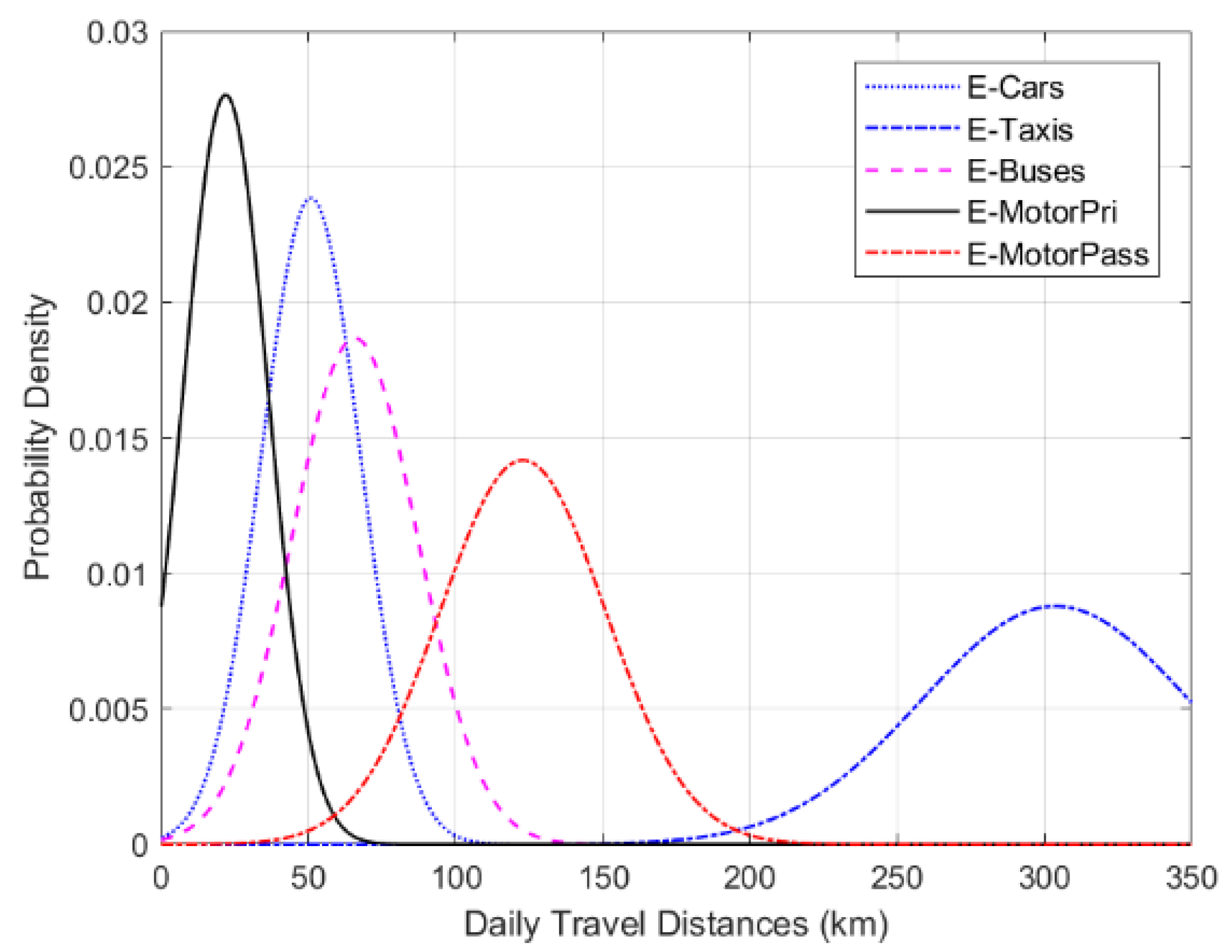
5.1. Daily Travel Distance

The daily travel distance on weekdays and weekends is considered to be the same in the simulation of EV charging demand. Due to the lack of statistics on the mileage of EVs, this paper assumes that EVs and conventional ICEVs have a similar daily mileage. The probability distributions of the daily travel distances of the EV fleet types based on the summary of the collected traffic data are shown in Figure 3.

The means and standard deviations of daily travel distances for E-Cars are given as 50.844 km and 16.724 km, respectively. In the case of the E-Taxis, the means and standard deviations of daily travel distances are 303.770 km and 45.405 km, respectively. The daily travel distances of E-Buses are relatively consistent due to their relatively regular daily routes. The probability distribution for mean and standard deviation are 65.729 km and 21.359 km, respectively. For E-MotorPri, the mean travel distance is 21.859 km, and the standard deviation is 14.422 km. The mean and standard deviation of daily travel distance for E-MotorPass is 122.851 km and 28.150 km, respectively.

The PDF types of EV daily travel distances $d_{i,j}$ are normal or logarithmic with a positive value of the travel distance. This can be calculated by Equations (1) and (2) replacing $x_{i,j}$ with $d_{i,j}$.

5.2. Driving Behaviors/Initial State of Charge

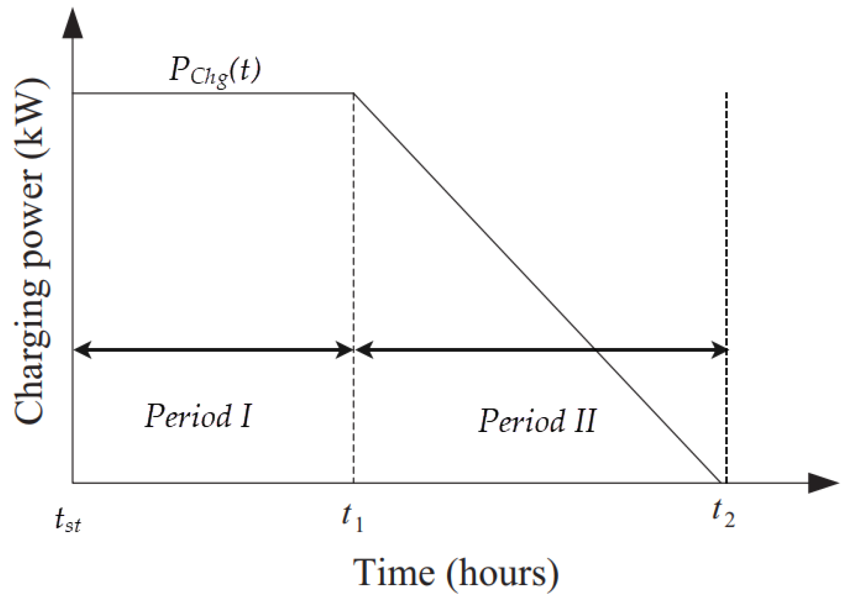
In this paper, in order to calculate the initial SOC of individual EVs arriving at home or the charging station, the driving behavior factors that affect fuel consumption are considered. These factors are randomly determined using the MCS and based on probability distributions of the transportation data and fed into the ANFIS model established in [18] in order to calculate the kWh/km fuel consumption of each EV. According to the fuel consumption model, three factors are identified for E-Cars that affect fuel consumption: vehicle size, driving speed, and the number of passengers. The probability distributions of these factors are considered based on the traffic surveyed data and tested-driving data, as shown in Figure 4.

In Figure 4a, mean and standard deviation values of the vehicle size are 1.497 and 0.656, respectively. The mean and standard deviation values of 3.358 and 0.686 can be used to categorize the driving speed into five levels as shown in Figure 4b. The number of passengers shown in Figure 4c is also categorized into five levels, with 1.976 and 1.003 as the mean and standard deviation, respectively. The PDFs of both vehicle size and number of passengers are lognormally distributed, while the PDF of travel speed is normally distributed. The mean values and standard deviations for various EV types are shown in

Table 3. Characteristic of PDFs for fuel consumption evaluation.

EV Types	Input1 (I1) (Vehicle Size)	Input2 (I2) (Driving Speed)	Input3 (I2) (No. Passenger)
E-Cars	L (1.497, 0.656)	N (3.358, 0.686)	L (1.976, 1.003)
E-Taxis	L (1.759, 0.836)	N (3.132, 0.461)	N (2.671, 1.070)
E-Buses	-	N (3.002, 1.047)	N (3.481, 0.786)
E-MotorPri	N (2.107, 0.656)	L (3.960, 1.120)	L (1.621, 0.684)
E-MotorPass	L (1.818, 0.428)	N (3.611, 1.019)	L (2.107, 0.310)

$N\left(\mu ,\sigma \right)$: normal PDF. $L\left(\mu ,\sigma \right)$: logarithmic PDF.

.

According to three inputs of E-Cars: assuming the three coefficients for three inputs are ${\alpha }_i, {\beta }_i, {\delta }_i$, and the constant is${\epsilon }_i$, the output of ith rule will be as follows:

If vehicle type is I₁, driving speed is I₂, and number of passengers is I₃, then

$$O_i^{}={\alpha }_i\times I_1+{\beta }_i\times I_2+{\delta }_i\times I_3+{\epsilon }_i$$

(3)

where $I_1,I_2,I_3$ are the linguistic labels of membership and functions for each input variable and $O_i$is the output in the ith rule.

Three inputs of the ANFIS model are randomly determined using the above PDFs, and then the fuel consumption of each EV $(F{C}_{E{V}_{i,j}})$ is estimated, as seen in Figure 5.

The PDF type of inputs of the ANFIS model $I_{i,j,n}$ are normal or logarithmic with a positive value assigned in Table 3. This can be calculated by Equations (1) and (2), replacing $x_{i,j}$ with $I_{i,j,n}$.

Fuel consumption $F{C}_{E{V}_{i,j}}$ evaluated by ANFIS model of different EV models using MATLAB programming with fuzzy toolbox, is used to calculate the initial SOC. The initial SOC of EV represents in $SO{C}_{i,j}$ can be estimated by Equation (4).

$$SO{C}_{i,j}^{}=1-\frac{d_{{}_{i,j}}^{}\times F{C}_{E{V}_{i,j}}^{}}{Ca{p}_{i,j}\times {\eta }_1^y}$$

(4)

where $d_{i,j}$ is daily travel distance of ith EV in jth fleet type calculated by using Equation (1) or Equation (2), $Ca{p}_{i,j}$ is the battery capacity, represented in terms of vehicle size (kWh). Several studies have been conducted on the efficiency of EV powertrains, including the depletion of battery power during driving cycles and the battery life cycles [22,23]. In this simulation, the loss of battery power during EV operation was considered by ${\eta }_1^y$as 0.95. For the lifetime of a battery, the battery efficiency depends on the ambient temperature and the state of charge, which decreases by about 20.0% over the total mileage of about 225,000 km or 900 charging cycles for the lithium-ion battery type [24]. Therefore, in the annual evaluation of the battery SOC in this study, it was assumed that the efficiency of the battery decreases by one percent per year.

5.3. Charging Power

Most EVs use conductive coupling to provide power for charging. There are mode 1, mode 2, mode 3 and mode 4 for conductive charging of e-vehicles [25]. In this paper, only the following two technologies are discussed:

• Slow charging: This is generally an AC system with low power. The recharging time is about 4–12 h [26]. Currently, slow charging technology is limited by onboard charging, which is designed by each vehicle manufacturer. The onboard charging power rating is provided in Table 1. Slow charging is generally occurred in modes 1 and 2.
• Fast charging: For mode 3 and mode 4, fast charging refers to a high-current AC system and a high-current DC system with a high-power output. It is a 20-min to 2-h charging service provided by a large current in an EV. Fast charging and charging stations currently on the market include power ratings from 22 kW to 43 kW for mode 3 and 50 kW, 100 kW and 150 kW for mode 4. The maximum power limit for EV fast charging is not considered in this simulation.

Generally, most EVs are charged overnight at a slow charging station when they arrive home after the last trip of the day. On the other hand, EV drivers choose fast charging when they charge at public location during the day. EVs that are charging at home are expected to utilize modes 1 and 2 to charge their batteries using onboard charging power. EVs charging at public charging stations, on the other hand, employ modes 3 and 4 for fast charging. The charging power used in this simulation can be seen in Table 1.

EV charging profiles may differ, depending on a number of factors, including battery type, charging location, and power distribution limitation. In this study, the batteries in EVs are assumed to be lithium-ion batteries, and the charging process follows a standard charging curve with two periods: a constant power period I and a descending power period II [27]. The primary objective is to investigate the increasing load demand for EV battery charging. For simplicity, a generalized model of EV charging profiles based on real data is adopted by linearizing the charging profile piecewise [28,29,30]; the charging profile is shown in Figure 6.

As shown in Figure 6, the charger operates at the rated current while the battery SOC is low, allowing a significant percentage of the battery charge to be recovered within the first few hours of charging. This continues until the battery voltage reaches its maximum limit, whereupon the charger maintains a constant voltage and reduces the current. In this model, period I is assumed to take 50.0% of the time to fully charge, while period II lasts for the remaining time duration, and it is assumed that the SOC of EV at the end of period I is 0.8. The mathematical expression for the charging power $P_{Chg}$ at time t is Equation (5):

$$P_{Ch{g}_{i,j}}(t)=\{\begin{array}{l}{P}_{\max }\hspace{0.17em}\hspace{0.17em}\hspace{0.17em}\hspace{0.17em}\hspace{0.17em}\hspace{0.17em}\hspace{0.17em}\hspace{0.17em}\hspace{0.17em}\hspace{0.17em}\hspace{0.17em}\hspace{0.17em}\hspace{0.17em}\hspace{0.17em}\hspace{0.17em};t_{s{t}_{i,j}}\le t\le t_1\\ P_{\max }\frac{(t_2-t)}{(t_2-t_1)}\hspace{0.17em}\hspace{0.17em}\hspace{0.17em}\hspace{0.17em}\hspace{0.17em}\hspace{0.17em}\hspace{0.17em};t_1\le t\le t_2\end{array}$$

(5)

where $t_1$ and $t_2$ are time instants that define the magnitude differences in charging power at time$t$. The charging power depends on the charging station of the EV. In this study, the charging power is randomly determined, based on the charging location.

5.4. Charging Strategy

The uncertainties of starting and recharging time are expressed in the charging behavior of EVs mainly by random method based on the statistical probability of driving behavior from multiple reviews. About 80.0% of the E-Cars were parked at private houses overnight [31]. The assumptions in this simulation are that 80.0% of the private EVs are plugged in during non-working hours (18:00–07:00), while the remaining 20.0% are charged during working hours (09:00–17:00). The start charging time for non-working hours is randomly determined using a normal distribution function with a mean of 18.5 and a deviation of 1, while a normal distribution function with a mean of 9 and a deviation of 0.9 is also used for working hours. Commercial EVs (E-Taxis) is typically operated in three shifts per day: 00:00–09:00, 09:00–16:00 and 16:00–24:00 reference in [32]. Since E-Taxis often have a high daily mileage, it is reasonable to predict that commercial E-Taxis will be charged in the fast charging mode, since the shorter charging time equates to more profitable hours of operation. E-Buses have well-defined schedules and routes as they are used to transport passengers in any organization, mostly in the morning before work hours and in the evening after work hours. They are usually charged with the fast charging mode during non-operating hours, and they are ready to be used again the next morning [33]. Due to a lack of data on the charging behavior of electric motorcycles, the charging behavior is assumed, based on the data collected in our previous study. For E-MotorPri, the daily mileage is quite low, and charging is usually done overnight at private residences. For E-MotorPass, it is assumed that daily driving patterns are organized into three-time shifts: 06:00–12:00, 12:00–18:00, and 18:00–24:00. In order not to lose the opportunity to provide services, it is assumed that each E-MotorPass contains a spare battery for battery replacement or battery swapping, with the other battery being charged while the driver is on the road. The start charging time $t_{s{t}_{i,j}}$ can be determined based on the PDF with a normal distribution type, which can be expressed by Equation (1) replacing $x_{i,j}$ with $t_{s{t}_{i,j}}$. The corresponding mean values and standard deviations for the start charging time are defined in

Table 4. Electric vehicle charging parameters for Monte-Carlo simulation.

EV Types	Charging Period	Charging Mode	Probability	Initial Daily Distance	Plug-In Time
E-Cars	09:00–17:00	Slow	10%	N (50.844, 16.724)	N (9, 0.9)
	09:00–17:00	Fast	10%		N (9, 0.9)
	18:00–07:00	Slow	80%		N (18.5, 1)
E-Taxis	00:00–09:00	Fast	90%	L (303.770, 45.405)	N (4, 2.5)
	09:00–16:00	Fast	60%		N (12, 2.5)
	16:00–24:00	Fast	50%		N (18, 1.5)
E-Buses	20:00–07:00	Fast	100%	N (65.729, 21.359)	N (20, 0.5)
E-MotorPri	18:00–07:00	Slow	80%	L (21.859, 14.422)	N (18.5, 1)
	09:00–17:00	Slow	20%		N (9, 1)
E-MotorPass	06:00–12:00	Slow	90%	N (122.851, 28.150)	N (9, 1.5)
	12:00–18:00	Slow	60%		N (15, 1.5)
	18:00–24.00	Slow	50%		N (21, 1.5)

$N\left(\mu ,\sigma \right)$: normal PDF. $L\left(\mu ,\sigma \right)$: logarithmic PDF.

.

5.4.1. Free-Charging Strategy

It is assumed that EV owners in this situation have no incentive to avoid peak charging. In this “worst case” situation, heavy simultaneous charging of EVs is simulated. Half of all EVs are charged almost at the same time while the remaining are charged normally. The total charging power at time t can be calculated using the EV charging parameters given in Table 4 and the start charging time can be determined in Equation (1).

5.4.2. Off-Peak Charging Strategy

In this charging strategy, a time-of-use (TOU) electricity tariff structure is adopted to represent the availability of new schemes to promote EV owners to charge their cars during off-peak hours and the possibility that additional schemes will be introduced. In this study, the peak load period is defined as 09:00 to 22:00, and the off-peak period is defined as 22:00 to 09:00.

E-Cars, E-Buses, and E-MotorPri have higher charging flexibility at night, according to empirical estimates. On the other hand, E-Taxis and E-MotorPasses need to be fully charged in the shortest possible time frame to prepare for the next driving activity and need to be charged at public charging stations. As such, they are not included in charging strategies. A uniform discrete distribution for off-peak charging of EV is used to account for the effect of the TOU electricity tariff on the battery charging start time. The charging situation is understood to be that half of all EVs are charged at almost the same time, while the rest are charged normally. The distribution of the start charging time for EVs charged overnight can be expressed by Equation (6).

$$f(t_{s{t}_{i,j}})=\{\begin{array}{l}0.8\hspace{0.17em}\hspace{0.17em}\hspace{0.17em}\hspace{0.17em}\hspace{0.17em}\hspace{0.17em}\hspace{0.17em}t\ge 22\\ 0.2\hspace{0.17em}\hspace{0.17em}\hspace{0.17em}\hspace{0.17em}\hspace{0.17em}\hspace{0.17em}\hspace{0.17em}t\ge 18\\ 0\hspace{0.17em}\hspace{0.17em}\hspace{0.17em}\hspace{0.17em}\hspace{0.17em}\hspace{0.17em}\hspace{0.17em}\hspace{0.17em}\hspace{0.17em}t=anyothertimes\end{array}\hspace{0.17em}\hspace{0.17em}\hspace{0.17em}\hspace{0.17em}\hspace{0.17em}(1\le t\le 24)$$

(6)

The TOU electricity tariff structure is assumed to influence the driver’s charging incentive during off-peak hours in this study but is not 100% effective in motivating changes to charging behavior in reality. In this simulation is assumed that 80.0% of vehicles are charged during off-peak hours, while the remaining vehicles are charged after 18:00. The total charging power at time t can be calculated using the EV charging parameters for probabilistic modelling given in Table 4 and Equation (6), incorporating the start charging time that is given in Equation (1).

5.5. Electric Vehicle Charging Demand Calculation

In order to calculate the impact of EV penetration, three main aspects are examined, consisting of the reduction of energy consumption, the reduction of GHGs, and the increase in load demands. These figures are calculated based on Energy Development Plan 2019–2036 and need to be reviewed annually.

When the charging uncertainties are completely determined, these parameters are used to calculate the EV charging demand, energy requirement and GHG emissions. The charging duration $t_{d_{i,j}}$ is related to the SOC, battery capacity $Ca{p}_{i,j}$ and charging power $P_{Ch{g}_{i,j}}$, and charging efficiency ${\eta }_2$ is 0.95 in all cases, which is double the duration of the first period $t_1$. The charging time duration of period I can be expressed using Equation (7):

$$t_1=\frac{(0.8-SO{C}_{i,j})\times Ca{p}_{i,j}}{P_{ch{g}_{i,j}}(t)\times {\eta }_2}$$

(7)

The discharge time of EV can be calculated in Equation (8):

$$t_{e_{i,j}}=t_{s{t}_{i,j}}+t_{d_{i,j}}$$

(8)

The EV charging demand of ith EV in jth fleet type is described in Equation (9):

$$P_{E{V}_{i,j}}(t)=\{\begin{array}{l}{P}_{Ch{g}_{i,j}}(t)\hspace{0.17em}\hspace{0.17em}\hspace{0.17em}\hspace{0.17em}\hspace{0.17em}\hspace{0.17em}\hspace{0.17em}\hspace{0.17em};t_{s{t}_{i,j}}\le t\le t_{e_{i,j}}\\ 0\hspace{0.17em}\hspace{0.17em}\hspace{0.17em}\hspace{0.17em}\hspace{0.17em}\hspace{0.17em}\hspace{0.17em}\hspace{0.17em}\hspace{0.17em}\hspace{0.17em}\hspace{0.17em}\hspace{0.17em}\hspace{0.17em}\hspace{0.17em}\hspace{0.17em}\hspace{0.17em}\hspace{0.17em}\hspace{0.17em};other\end{array}$$

(9)

The aggregated charging demand in year yth of the total EVs $N_j$ at different times t should be expressed in Equation (10):

$$P_{EV}^y(t)={\displaystyle \sum _{j=1}^5{\displaystyle \sum _{i=1}^{N_j}{P}_{E{V}_{i,j}}(t)}}$$

(10)

5.6. Energy Consumption and Greenhouse Gases Emissions Calculation

The energy consumption of ICEVs in year yth is investigated in order to calculate the energy reduction of replacement ICEVs by EVs, which can be expressed by Equation (11):

$$E_{ICEV}^y={\displaystyle \sum _{j=1}^5{\displaystyle \sum _{i=1}^{N_j^y}{\displaystyle \sum _{k=1}^{365}{d}_{i,j}\times F{C}_{{}_{ICE{V}_{i,j}}}^{}}}}$$

(11)

where $d_{i,j}$ is daily travel distance of ith EV in jth fleet type, and $F{C}_{ICE{V}_{i,j}}$ is fuel consumption per distance of ith ICEVs in jth fleet type.

The daily energy requirement when charged EV of ith EV in jth fleet type can be calculated in Equation (12):

$$E_{E{V}_{i,j}}=\frac{(1-SO{C}_{i,j})\times Ca{p}_{i,j}}{{\eta }_1^y}$$

(12)

The total energy requirement of EV charging demand in year yth should be expressed in Equation (13):

$$E_{EV}^y={\displaystyle \sum _{j=1}^5{\displaystyle \sum _{i=1}^{N_j}{\displaystyle \sum _{k=1}^{365}{E}_{E{V}_{i,j}}}}}$$

(13)

The energy reduction in year yth should be expressed in Equation (14):

$$E_R^y=E_{ICEV}^y-E_{EV}^y$$

(14)

The annual GHG emissions in year yth released from ICEVs in transport sector can be expressed in Equation (15):

$$GH{G}_{ICEV}^y=E_{ICEV}^y\times GH{G}_{f_{ICEV}}$$

(15)

where $GH{G}_{f_{ICEV}}$ is the factor of CO₂ emissions emitted from ICEVs tailpipe in transport sector based on 2019 Thailand energy consumption statistics report, which is specified as instant value by 1.86 ktCO₂/ktoe.

Equation (16) can be used to estimate annual GHG emissions in year yth for electricity generation to provide EV charging:

$$GH{G}_{EV}^y=E_{EV}^y\times GH{G}_{f_{EV}}$$

(16)

where $GH{G}_{f_{EV}}$ is the factor of CO₂ emissions released from electricity generation process based on 2019 Thailand energy consumption statistics report, which is specified as instant value by 0.486 kg CO₂/kWh.

Therefore, the reduction of GHG emissions in the transport sector in year yth can be expressed in Equation (17):

$$GH{G}_R^y=GH{G}_{ICEV}^y-GH{G}_{EV}^y$$

(17)

5.7. Analysis Frameworks of Benefits and Trade-Offs for EV Charging

In the MCS, the daily travel distance, fuel consumption, initial SOC, start charging time, and charging power are a set of independent stochastic variables for each EV, produced using the preceding section’s modeling parameters. The MCS process is presented in Figure 7. The EV charging demand based on MCS can be described in the following steps:

1.

Initiate number of EVs: The EV penetration in each year yth is assigned.

2.

Based on the PDFs of stochastic variables, daily travel distance $d_{i,j}$ of ith EV in jth fleet type is generated by Equation (1) or (2) for normal or logarithmic distribution type, respectively.

3.

In order to evaluate the fuel consumption of individual EVs, inputs of ANFIS model are generated as shown in Figure 5. (The number of inputs depends on the vehicle type, which is shown in Table 2).

4.

The initial state of charge can be estimated by Equation (4).

5.

Charging power is randomly determined based on the charging location, as expressed in Equation (5).

6.

Start charging time is generated based on the PDF of each EV type, which can be expressed in Equation (1). In this step, charging strategies are considered.

7.

The aggregated EV charging demand, energy requirement and GHG emissions can be calculated by Equations (7)–(17). Loop counts continue until the total EV calculation is completed, representing the total number of EVs.

8.

The simulation runs from 2019 to 2036 and has 100 iterations per year.

6. Results and Discussion

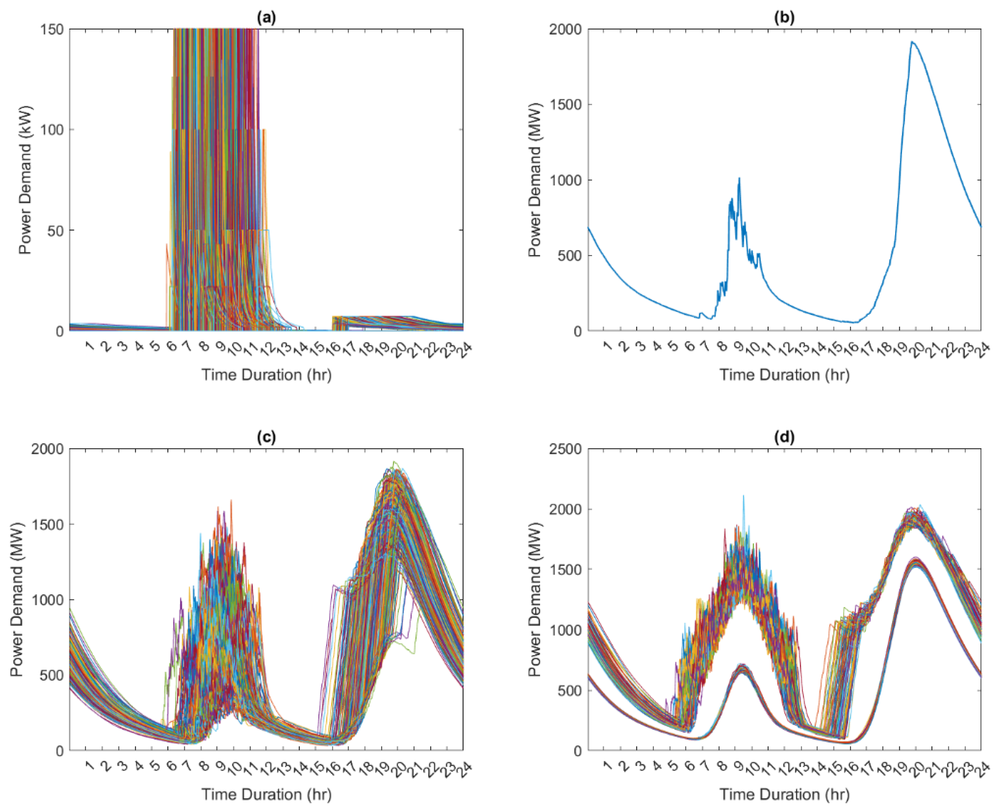
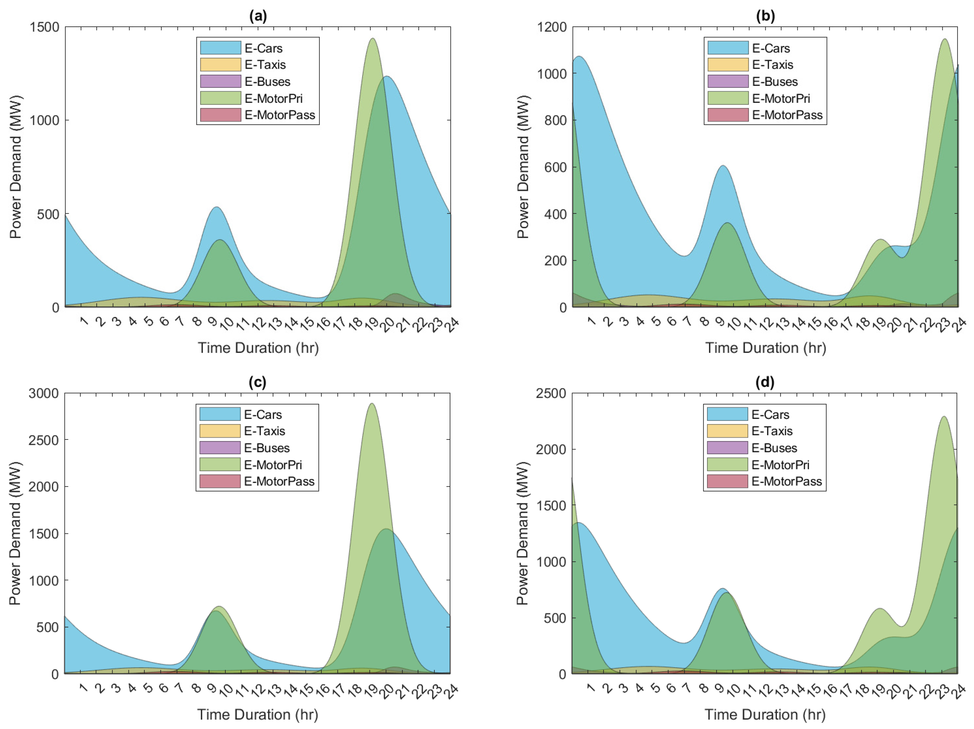
6.1. Electric Vehicle Charging Demand

The daily charging demand of each EV was calculated based on the daily travel distance, relative to the SOC. To simplify the calculation, one day is treated as a period, and one day is divided into 1440 periods. When the EVs were connected to the grid, the charging power of each minute was recorded and added together to find the overall charging power of all the EVs. Thus, the metric data of the total EV charging demand for a year is obtained by 365 rows and 1440 columns; however, the results were presented in 24 h a day for easy understanding. To ensure the accuracy and stability of the model, the simulation of EV charging demand was performed in 100 iterations.

In the EV charging simulation, daily charging was not taken into account because some EVs have very low mileage or were not used at all during the day, making daily charging unnecessary. The charging event of an EV was determined by the SOC, which was calculated based on the cumulative daily mileage. The charging event was determined by taking into account the user’s charging decisions, which were randomly determined following a uniform distribution between the SOC value of 0.2 and 0.5. The EV was connected to the grid if the calculated SOC value was less than the SOC value selected by the random method. In contrast, some EVs are not charged because the daily distance driven is extremely low, so the cumulative mileage is combined with the next day’s mileage. Where the daily mileage was very high and the calculated battery SOC showed negative values, charging was determined to have occurred more than once per day.

To explain the EV charging simulation, an extreme EV penetration scenario with a free charging strategy for the E-Cars fleet type was examined, as shown in Figure 8. Figure 8a shows the daily charging profile of the entire E-Cars fleet in 2036, where the highest charging power is 150 kW from the fast-charging station. From the figure, one line graph represents the daily charging demand of each EV (1.35 million EVs). However, Figure 8a shows less than 1.35 million EVs because some EVs do not need to be charged every day. Figure 8b shows the single snapshot of an aggregated daily load profile of the E-Cars fleet in 2036. In this snapshot, the peak occurred in the early evening and is about 1915 MW. According to the charging demand in the first iteration, Figure 8c shows one of a hundred potential iterations of the EV fleet charging demand calculation in 2036. Figure 8c includes 365-line graphs, where one line graph represents the aggregate daily load profile of the E-Car fleet. The level of daily load demand was varied depending on the daily mileage, fuel consumption, SOC before charging, and charging power, as shown in the figure. Figure 8d depicts the mean and maximum charging profile of the EV charging simulation after one hundred iterations. The figure includes the mean and maximum values of each 100 lines (one line represents one iteration of the simulation), each representing the average or maximum daily load demand for 365 days. From the daily mean and maximum of charging profile, it can be seen that the variance of the simulated demand is relatively high and, when used to assess the impact of EV charging, the results may be inaccurate. Therefore, the boxplot of the simulated EV charging load profile with two charging strategies and EV penetration scenarios were analyzed.

The simulated results of the EV charging profile of five vehicle fleet types for two different charging strategies in 2036 are shown in Figure 9. The results of EV charging demand for the worst-case scenario (the free charging strategy), in which the probable EV penetration scenario is considered, is shown in Figure 9a. It can be clearly seen in the figure that the peak demand was caused to the greatest extent by E-MotorPri, followed by E-Cars. The peak demand from the battery charge occurs in the early evening, due to the fact that most people recharge immediately when they arrive at a private residence. Such a significant increase in charging demand will significantly impact on peak electricity demand. To avoid impact on the local distribution network and installed generation capacity due to EV charging demands, the off-peak charging strategy based on the TOU electricity tariff structure is another option that may motivate EV users to change their charging behavior. The EV charging demand for the off-peak charging strategy, in which the probable EV penetration scenario is considered, is shown in Figure 9b. It can be seen that the peak demand has changed compared to the free charging strategy that occurred before midnight, and E-MotorPri is still the type of vehicle that presents the highest demand. Figure 9c,d show the EV charging in the extreme EV penetration scenario under the free charging and the off-peak charging strategy, respectively.

Figure 10 shows the boxplot of EV charging demand in 2036 for two charging strategies, considering two EV penetration scenarios. Because the results of the EV charging demand were represented in the daily load profile point of view, while the simulation of EV charging demand was conducted for a year, the simulation was performed in 100 iterations. Therefore, the boxplot is an adequate tool for presenting the simulation results because the boxplot represents the overall simulation results, including the mean, minimum, and maximum values. In addition, the boxplot also shows the variance of EV charging demand at any point, and the outlier of the data was also displayed as a symbol over and under the maximum and minimum values, respectively. Figure 10a shows the boxplot of EV charging demand for the probable scenario of EV penetration under the free charging strategy. Peak demand in this situation was approximately 3500 MW and occurred around 20:00. On the other hand, with the same EV penetration level, peak demand dropped to nearly 3000 MW before midnight under the off-peak charging strategy, as shown in Figure 10b. According to the extreme scenario of EV penetration under the free charging strategy, as shown in Figure 10c, the peak demand happened at 20:00, as in the probable scenario, but the peak demand was almost double that, at about 6000 MW. In the case of the off-peak charging strategy, peak demand—compared with the free charging strategy—decreased by about 16.0%, which occurred near to midnight, as shown in Figure 10d.

The daily load profile in 2036 was generated based on the daily load profile from 2019, as shown in Figure 11. From the figure, the blue area represents a daily load profile in 2036 with the EV charging demand box plotted and the blue line represents the spinning reserve. In addition, the charging demand as shown in the boxplot also shows the outlier value. Figure 11a shows the daily load profile with EV charging demand for the probable scenario of EV penetration under the free charging strategy. It is found that the increased demand exceeded the calculated spinning reserve at 18:00 and the system peak demand has been changed to 20:00. According to all of the experiment points, it was found that the peak demand occurs during working hours at 14:30, due to the fast-charging station. However, the boxplot can point out that the peak demand is an outlier value that occurs only a few times across all experiment points. Therefore, it is not necessary to consider such values. In the case of the off-peak charging strategy, as shown in Figure 11b, this strategy could reduce the peak demand during peak hours, as compared to the free charging strategy, but this leads to a new peak which occurs around 23:00, and the charging demand could cause the system peak to exceed the spinning reserve. Figure 11c shows the daily load profile in 2036 with the EV charging demand for the extreme scenario of EV penetration under the free charging strategy. The boxplot shows that the maximum values of EV charging demand increased the system load to close to the spinning reserve at 08:30 and the load demand began to exceed the spinning reserve from 17:00 to 22:00. After this, the load demand returned to a normal state. As a result of this situation, the system’s peak demand occurred at 20:00, and the peak value was about 55,000 MW. The additional EV charging demand for the extreme scenario of EV penetration under the off-peak charging strategy can be seen in Figure 11d. In this charging strategy, EV charging demand has led to a new peak in the system load, with the peak occurring in the hours before midnight; at around 23:00. In fact, the additional demand can increase the load factor by filling some areas of the valley during off-peak hours. However, under the off-peak scenario, between 20:00 and 02:00, the system load has significantly increased.

The statistical analysis for 2036, represented in the boxplot shown in Figure 12, demonstrates the effectiveness levels of two charging strategies. In the case of the probable scenario of EV penetration, the off-peak charging strategy achieves a better performance than the free charging strategy for reducing the peak demand during peak hours. In the case of the extreme scenario of EV penetration, the off-peak charging strategy cannot reduce the system peak load because this charging strategy creates a new peak before midnight. However, it can reduce the peak load during working hours and increase the load factor during off-peak hours. In addition, the off-peak charging strategy has a power variance range between 38,950 MW and 55,900 MW. In 2036, according to a peak demand of baseload, peak demand that results from EV charging demand for the probable and extreme scenarios of EV penetration under free charging strategy was increased by approximately 4.1% and 7.2%, respectively. For the off-peak charging strategy, the increase in peak demand for the probable and extreme scenarios of EV penetration was about 3.7% and 7.5%, respectively.

From the above-simulated results, the increased load from EV charging demand in all situations remained inside the safety margin, compared to the installed generation capacity in PDP2018r1. Nevertheless, it can be clearly seen that the increased load demand due to all EV charging strategies has a direct impact on the power generation system as the spinning reserve cannot respond to the additional load. This impact can also cause concern for the distribution system operators, and it can reduce system reliability. EVs, on the other hand, might present a potential advantage to the power system by offering vehicle-to-grid (V2G) services when parked and not being driven, giving grid operators more flexibility in terms of the EV charging schedule. Among these functions, V2G can serve as an energy storage device that may be charged during off-peak hours and discharged during peak hours, as well as providing auxiliary services such as spinning reserves [34].

Through the introduction of a TOU electricity tariff structure, the off-peak charging strategy that incentivizes changes in charging behavior, peak demand during peak hours can be effectively reduced and the valley can be filled during low system loads. However, the off-peak charging strategy can cause a new peak load demand, which may affect the startup and shutdown process of each generation unit. Therefore, it is necessary to consider the implementation pathways for supporting new peak loads. Both the Unit Commitment and Economic Dispatch have been investigated in order to respond appropriately and efficiently to simultaneous charging.

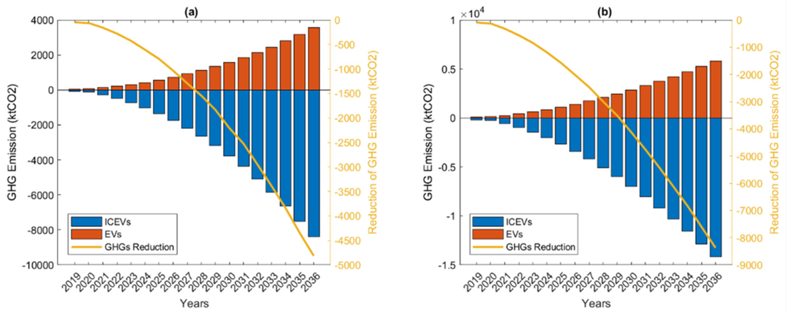
6.2. Energy Consumption and Greenhouse Gases Emissions

In order to present the benefits of EV technology, the comparison of energy consumption between conventional vehicles and EVs was investigated, and the energy consumption was presented in terajoules (TJ), as shown in Figure 13. The energy consumption was related to the charging behavior, and the energy of the two charging strategies was the same. The calculated results of energy consumption based on the EV penetration scenarios for the probable and extreme cases are shown in Figure 13a,b, respectively. The green bars at the top area indicate the energy consumption obtained from EV charging, whereas the blue bars at the bottom area indicate the energy consumption of ICEVs. The reduction of energy consumption by the replacement of ICEVs with EVs is represented in the red line. In the case of probable EV penetration, by 2036, energy consumption could be reduced by approximately 156,000 TJ. Whereas the extreme case of EV penetration could be reduced energy consumption by nearly 260,000 TJ.

In 2036, the energy demand for EV charging was about 7000 GWh and 12,500 GWh for the probable and extreme EV penetration scenarios, respectively, which was about 2.0% and 3.5% compared to the energy demand forecasted for 2036 in the PDP2018r1. According to Thailand’s Energy Efficiency Plan 2015 (EEP2015), the transportation sector’s target for improve energy efficiency by reducing energy consumption is expected to be 30,213 ktoe (equivalent to approximately 1,265,000 TJ) by 2036, of which 1123 ktoe, or approximately 47,000 TJ, is accounted for by EV technology, and assuming that there are only 1.2 million passenger cars. In comparison, the reduction of energy consumption for probable and extreme EV penetration scenarios was about 12.7% and 21.7%, respectively, compared to the transport energy efficiency target.

One of the most important reasons to replace ICEVs with EVs is to reduce greenhouse gas emissions. With the exception of electricity from alternative energy sources, such as hydro, solar, nuclear, biomass, and wind, EVs do not produce tailpipe pollutants; nevertheless, power plants that generate electricity to fuel EVs still release GHGs [35]. In this study, a simplification of the environmental impact assessment is used to provide an overview of transport emissions. Therefore, carbon dioxide equivalent (CO₂eq) was presented as the global warming potential (GWP) of various greenhouse gases emissions. The CO₂eq value used in this simulation is 0.486 kgCO₂ per kWh of electricity generated by power plants, which was referred in Section 5.6. The calculated results of CO₂ emissions are shown in Figure 14. The overall CO₂ emissions for the probable and extreme scenarios of EV penetration can be seen in Figure 14a,b, respectively. From the figures, by 2036, CO₂ emissions from electricity generation in both scenarios accounted for nearly a half of the reduced emissions achieved by replacing conventional vehicles with EVs. The reduction of CO₂ emissions in the transport sector for the probable and extreme EV penetration scenarios was approximately 4800 ktCO₂ and 8370 ktCO₂, respectively.

According to the department of land transport’s annual report, the amount of pollution recorded in 2018 was 67,900 ktCO₂ [36]. In comparison, the reduction in CO₂ emissions by 2036 for both the probable and extreme EV penetration scenarios was about 7.0% and 12.0%, respectively, compared with the CO₂ emissions of the transport sector in 2018.

7. Conclusions

In this paper, stochastic modelling based on Monte-Carlo simulation is presented in order to analyze the benefits and trade-offs for EV penetration in Thai road transport. Several uncertainty factors that may affect EV charging profiles are considered. The proposed model focuses on the randomness and heterogeneous characteristics of driving behavior and EV charging parameters in order to represent the variance and unpredictability of EV charging demand under two charging strategies: a free charging and an off-peak charging strategy. Furthermore, the evaluation of the daily load profiles at the national level with EV charging demand indicates the adequacy of the installed generation capacity in Thailand, based on EV penetration scenarios. In terms of a perspective that takes into account the benefits of EV adoption, the reduction of energy consumption and greenhouse gases emission is introduced; whereas the increase of EV charging demand is presented as a trade-off perspective. The adoption of EV technology in Thai road transport can reduce both energy consumption and greenhouse gas emissions. However, the amount of pollutants emitted by the generation of electricity to supply EVs charging is equivalent to nearly half the amount of tailpipe pollutants produced by conventional vehicles. Furthermore, such problems can be solved with the use of alternative energy sources, such as nuclear power, biomass, water, solar, and wind. According to EV charging demand, heavy simultaneous charging of EVs for the residential sector under the free charging strategy has led to peaks in the early evening, when most EV users have arrived at their private residence and immediately connect their EVs to the grid. The off-peak charging strategy, based on the TOU electricity tariff structure, can effectively reduce the system peak load and can also increase the system load factor. The increased load from EV charging demand in all scenarios remains inside the safety margin compared to the installed generation capacity in PDP2018r1. Nevertheless, the increased load demand due to all EV charging strategies has a direct impact on the power generation system, because the spinning reserve cannot respond to the additional load and the off-peak charging strategy causes a new load peak in the system before midnight.

The proposed model is more flexible than the previously developed model mentioned in the introduction section, which demonstrates that the different charging behavior of EV users affects the variance of charging demand. According to the simulation results represented in the block diagram, it can be seen that the power demand at certain times is greater than the system’s spinning reserve. If we only consider the average value of the variance of the charging demand, it may be inaccurate in predicting the potential load of EV charging. The developed model can effectively support the cross-sector analysis (transportation and utility sectors) to manage the unpredictable loads of EV charging because the model is based on data about the driving behavior of real users and the configuration of uncertainty variables is widely covered by the modern data. However, the disadvantage of this model is that it requires a longer computational time. A future study will investigate how EV charging demand varies between weekdays and the weekend, as well as investigating a smart charging strategy intended to optimize the peak shaving and valley filling of the system load demand. Moreover, both the Unit Commitment and Economic Dispatch have been investigated according to the Power Development Plan for Thailand in order to respond appropriately and efficiently to simultaneous charging.

References

1. Energy Statistics of Thailand. Energy Policy and Planning Office, Ministry of Energy, Thailand. Available online: https://drive.google.com/file/d/1zhiH0TcZWUAuReQA_TPdCelhWjH3lTPP/view (accessed on 1 June 2021).
2. Tribioli, L.; Barbieri, M.; Capata, R.; Sciubba, E.; Jannelli, E.; Bella, G. A real time energy management strategy for plug-in hybrid electric vehicles based on optimal control theory. Energy Procedia 2014, 45, 949–958. [Google Scholar] [CrossRef]
3. Wróblewski, P.; Kupiec, J.; Drożdż, W.; Lewicki, W.; Jaworski, J. The Economic Aspect of Using Different Plug-In Hybrid Driving Techniques in Urban Conditions. Energies 2021, 14, 3543. [Google Scholar] [CrossRef]
4. Lian, J.; Liu, S.; Li, L.; Liu, X.; Zhou, Y.; Yang, F.; Yuan, L. A mixed logical dynamical-model predictive control (MLD-MPC) energy management control strategy for plug-in hybrid electric vehicles (PHEVs). Energies 2017, 10, 74. [Google Scholar] [CrossRef]
5. Chen, Y.; Hu, K.; Zhao, J.; Li, G.; Johnson, J.; Zietsman, J. In-use energy and CO2 emissions impact of a plug-in hybrid and battery electric vehicle based on real-world driving. Int. J. Environ. Sci. Technol. 2018, 15, 1001–1008. [Google Scholar] [CrossRef]
6. Targeting Electric Vehicles by 2030. Available online: https://thestandard.co/supattanapong-electric-vehicles-target-by-2030/ (accessed on 1 August 2021).
7. Energy Policy and Planning Office, Ministry of Energy, Thailand. Energy Efficiency Plan; EEP 2015. Available online: http://www.eppo.go.th/images/POLICY/PDF/EEP2015.pdf (accessed on 10 June 2021).
8. Daina, N.; Sivakumar, A.; Polak, J.W. Modelling electric vehicles use: A survey on the methods. Renew. Sustain. Energy Rev. 2017, 68, 447–460. [Google Scholar] [CrossRef] [Green Version]
9. Ni, X.; Lo, K.L. A Methodology to Model Daily Charging Load in the EV Charging Stations Based on Monte Carlo Simulation. In Proceedings of the 2020 International Conference on Smart Grid and Clean Energy Technologies (ICSGCE), Kuching, Malaysia, 4–7 October 2020; pp. 125–130. [Google Scholar] [CrossRef]
10. Liu, D.; Li, Z.; Jiang, J.; Cheng, X.; Wu, G. Electric Vehicle Load Forecast Based on Monte Carlo Algorithm. In Proceedings of the 2020 IEEE 9th Joint International Information Technology and Artificial Intelligence Conference (ITAIC), Chongqing, China, 11–13 December 2020; pp. 1760–1763. [Google Scholar] [CrossRef]
11. Guo, C.; Liu, D.; Geng, W.; Zhu, C.; Wang, X.; Cao, X. Modeling and Analysis of Electric Vehicle Charging Load in Residential Area. In Proceedings of the 2019 4th International Conference on Power and Renewable Energy (ICPRE), Chengdu, China, 21–23 September 2019; pp. 394–402. [Google Scholar] [CrossRef]
12. Singh, J.; Tiwari, R. Probabilistic Modeling and Analysis of Aggregated Electric Vehicle Charging Station Load on Distribution System. In Proceedings of the 2017 14th IEEE India Council International Conference (INDICON), Roorkee, India, 15–17 December 2017; pp. 1–6. [Google Scholar] [CrossRef]
13. Su, J.; Lie, T.T.; Zamora, R. Modelling of large-scale electric vehicles charging demand: A New Zealand case study. Electr. Power Syst. Res. Elsevier BV 2019, 167, 171–182. [Google Scholar] [CrossRef]
14. Moon, J.H.; Gwon, H.N.; Jo, G.R.; Choi, W.Y.; Kook, K.S. Stochastic Modeling Method of Plug-in Electric Vehicle Charging Demand for Korean Transmission System Planning. Energies 2020, 13, 4404. [Google Scholar] [CrossRef]
15. Foley, A.; Tyther, B.; Calnan, P.; Gallachóir, B.Ó. Impacts of Electric Vehicle charging under electricity market operations. Appl. Energy 2013, 101, 93–102. [Google Scholar] [CrossRef]
16. Saisirirat, P.; Chollacoop, N.; Tongroon, M.; Laoonual, Y.; Pongthanaisawan, J. Scenario analysis of electric vehicle technology penetration in Thailand: Comparisons of required electricity with power development plan and projections of fossil fuel and greenhouse gas reduction. Energy Procedia 2013, 34, 459–470. [Google Scholar] [CrossRef] [Green Version]
17. Department of Land Transport. Registered Car (Cumulative) in Transport Statistics Group Data. Available online: https://web.dlt.go.th/statistics/ (accessed on 1 June 2021).
18. Uthathip, N.; Bhasaputra, P.; Pattaraprakorn, W. Application of ANFIS Model for Thailand’s Electric Vehicle Consumption. Comput. Syst. Sci. Eng. 2021, in press. [Google Scholar] [CrossRef]
19. Suchart, P. Development of an Electric Bus Prototype Using Lithium-Ion Battery for Thailand. Ph.D. Dissertation, School of Electrical Engineering Institute of Engineering Suranaree University of Technology, Nakhon Ratchasima, Thailand, 2018. [Google Scholar]
20. Thailand Power Development Plan 2018–2037 (PDP 2018). The Government Policies of Electricity, Ministry of Energy, Thailand. Available online: https://www.thaienergy.org/Blog/5 (accessed on 10 June 2021).
21. Spinning Reserve. Electric Generating Authority of Thailand. Available online: https://www.egat.co.th/index.php?option=com_content&view=article&id=357&Itemid=2 (accessed on 1 May 2021).
22. Wu, J.; Liang, J.; Ruan, J.; Zhang, N.; Walker, P.D. Efficiency comparison of electric vehicles powertrains with dual motor and single motor input. Mech. Mach. Theory 2018, 128, 569–585. [Google Scholar] [CrossRef]
23. Kellner, Q.; Hosseinzadeh, E.; Chouchelamane, G.; Widanage, W.D.; Marco, J. Battery cycle life test development for high-performance electric vehicle applications. J. Energy Storage 2018, 15, 228–244. [Google Scholar] [CrossRef]
24. BU-1003a: Battery Aging in an Electric Vehicle (EV). Available online: https://batteryuniversity.com/article/bu-1003a-battery-aging-in-an-electric-vehicle-ev (accessed on 1 June 2021).
25. Qian, K.; Zhou, C.; Yuan, Y. Impacts of high penetration level of fully electric vehicles charging loads on the thermal ageing of power transformers. Int. J. Electr. Power Energy Syst. 2015, 65, 102–112. [Google Scholar] [CrossRef] [Green Version]
26. Xiang, K.; Li, Y.; Lin, C.; Li, Y.; Cai, Q.; Du, Y. In An Electric Vehicle Charging Load Forecast Model Based on Probability Distribution. In Proceedings of the 2020 IEEE 4th Conference on Energy Internet and Energy System Integration (EI2), Wuhan, China, 30 October–1 November 2020; pp. 2847–2851. [Google Scholar] [CrossRef]
27. Marra, F.; Yang, G.Y.; Træholt, C.; Larsen, E.; Rasmussen, C.N.; You, S. In Demand profile study of battery electric vehicle under different charging options. In Proceedings of the 2012 IEEE Power and Energy Society General Meeting, San Diego, CA, USA, 22–26 July 2012; pp. 1–7. [Google Scholar] [CrossRef] [Green Version]
28. Staats, P.T.; Grady, W.M.; Arapostathis, A.; Thallam, R.S. A statistical method for predicting the net harmonic currents generated by a concentration of electric vehicle battery chargers. IEEE Trans. Power Deliv. 1997, 12, 58–66. [Google Scholar] [CrossRef]
29. Gómez, J.C.; Morcos, M.M. Impact of EV battery chargers on the power quality of distribution systems. IEEE Trans. Power Deliv. 2003, 18, 975–981. [Google Scholar] [CrossRef]
30. Heydt, G.T. The impact of electric vehicle deployment on load management strategies. IEEE Trans. Power Appar. Syst. 1983, PAS-102, 1253–1259. [Google Scholar] [CrossRef]
31. Duncan, J. Electric Vehicles: Impacts on New Zealand’s Electricity System. 2010. Available online: https://ir.canterbury.ac.nz/handle/10092/11575 (accessed on 1 May 2021).
32. Charlton, S.G.; Baas, P.H.; Alley, B.D.; Luther, R.E. Analysis of Fatigue Levels in New Zealand Taxi and Local-Route Truck Drivers. 2003. Available online: https://www.nzta.govt.nz/resources/fatigue-levels-in-taxi-and-local-route-drivers/ (accessed on 1 May 2021).
33. New Zealand’s First Electric Bus Hits the Road. Auckland University of Technology. 2018. Available online: https://news.aut.ac.nz/around-aut-news/new-zealands-first-electric-bushits-the-road (accessed on 1 May 2021).
34. Sioshansi, R.; Denholm, P. The value of plug-in hybrid electric vehicles as grid resources. Energy J. 2010, 31, 1–23. [Google Scholar] [CrossRef] [Green Version]
35. Winyuchakrit, P.; Sukamongkol, Y.; Limmeechokchai, B. Do Electric Vehicles Really Reduce GHG Emissions in Thailand? Energy Procedia 2017, 138, 348–353. [Google Scholar] [CrossRef]
36. CO2 Emission by Energy Type and Sector. Available online: http://www.eppo.go.th/index.php/th/energy-information/static-energy/static-co2 (accessed on 1 June 2021).
Figure 1. EVs penetration scenarios of difference vehicle types: (a) Private EVs; (b) Taxi EVs; (c) Non-fixed route bus EVs; (d) Personal electric motorcycles; (e) Passenger electric motorcycles in case of probable scenario and (f) Passenger electric motorcycles in case of extreme scenario.
Energies 14 05037 g001
Figure 2. The daily load profile in 2019 and 2036.
Energies 14 05037 g002
Figure 3. Probability distributions of daily travel distances.
Energies 14 05037 g003
Figure 4. Probability distributions of input model for E-Cars: (a) Vehicle size; (b) Driving speed and (c) Number of passengers.
Energies 14 05037 g004
Figure 5. Evaluation of fuel consumption of each EV.
Energies 14 05037 g005
Figure 6. Charging characteristic of electric vehicle charger.
Energies 14 05037 g006
Figure 7. Analysis of benefits and trade-offs process for EV charging based on MCS.
Energies 14 05037 g007
Figure 8. Charging demand for extreme EV penetration scenario under free charging strategy for E-Cars: (a) Daily charging profile of the entire E-Cars fleet; (b) 365 daily load profiles; (c) Snapshot a daily charging demand; (d) Daily mean and daily maximum of charging profile.
Energies 14 05037 g008
Figure 9. Mean charging demand of five vehicle fleet types: (a) Free charging strategy (probable scenario); (b) Off-peak charging strategy (probable scenario); (c) Free charging strategy (extreme scenario) and (d) Off-peak charging strategy (extreme scenario).
Energies 14 05037 g009
Figure 10. Boxplot of EV Charging demand in 2036: (a) Free charging strategy (probable scenario); (b) Off-peak charging strategy (probable scenario); (c) Free charging strategy (extreme scenario) and (d) Off-peak charging strategy (extreme scenario).
Energies 14 05037 g010
Figure 11. Daily load profile in 2036 with EV charging demand: (a) Free charging strategy (probable scenario); (b) Off-peak charging strategy (probable scenario); (c) Free charging strategy (extreme scenario) and (d) Off-peak charging strategy (extreme scenario).
Energies 14 05037 g011
Figure 12. Boxplot of EV charging load profile in 2036 with two charging strategies.
Energies 14 05037 g012
Figure 13. Energy consumption of ICEVs and EVs in 2036 based on EV penetration scenarios: (a) Probable scenario and (b) Extreme scenario.
Energies 14 05037 g013
Figure 14. CO2 emissions generated by ICEVs and EVs based on EV penetration scenarios: (a) Probable scenario and (b) Extreme scenario.
Energies 14 05037 g014